Modeling Study on the Asymmetry of Positive and Negative Storm Surges along the Southeastern Coast of China

Abstract

In this paper, a three-dimensional storm surge model was developed based on the Finite Volume Community Ocean Model (FVCOM) by the hindcasts of four typhoon-induced storm surges (Chan-hom, Mireille, Herb, and Winnie). After model validation, a series of sensitivity experiments were conducted to explore the effects of key parameters in the wind and pressure field (forward speed, radius of maximum wind (RMW), inflow angle, and central pressure), typhoon path, wind intensity, and topography on the storm surge and surge asymmetry between sea level rise (positive surge) and fall (negative surge) along the southeastern coast of China (SCC). The model results show that lower central pressure and larger RMW could lead to stronger surge asymmetry. A larger inflow angle results in a stronger surge asymmetry. In addition, the path of Chan-hom is the most dangerous path type for the Zhoushan Archipelago area, and that of Winnie follows next. The model results also indicate that the non-linear interaction between wind field and pressure field tends to weaken the peak surge elevation. The effect of topography on storm surges indicates that the peak surge elevation and its occurrence time, as well as the surge asymmetry, increase with a decreasing slope along the SCC.

1. Introduction

A storm surge is an abnormal rise of sea surface elevation, which is commonly induced by a tropical cyclone or a typhoon. The severity of a storm surge is affected by many factors, including the intensity, size, path, and forward speed of a storm, the shallowness of bathymetry, as well as the interaction with astronomical tides, especially when it coincides with high spring tide or low neap tide [1,2,3,4,5]. Previous studies have shown that the non-linear interaction of tide and surge may lead to both reduction and amplification of surge elevation depending on the tidal phases during storm landfall, and generally increasing the surge elevation at rising tide and decreasing the surge height at high tide [6,7,8]. Storm surge has potentially destructive effects, causing heavy losses of lives and property and changing the ocean environment [9,10]. Besides, affected by global climate change, coastal communities are becoming more vulnerable to storm surges [11,12,13,14]. For example, Woth et al. [12] found that under climatic conditions, storm surge extremes may increase along the North Sea coast at the end of this century. Rahmstorf [14] showed that with the global warming, the intensification of tropical storms can be expected, leading to an increase of flood risks to coastal communities. In recent years, the Ensemble Prediction System (EPS) technique has been applied to predict the evolution of storm surges [15,16,17]. It has been operationally used by different agencies, such as the UK Environment Agency, the Storm Surge Warning Service of Rijkswaterstaat, and Water Management Authority in Netherlands. The main advantage of the EPS technique is the production of information on forecast uncertainty, and it can work by running several forecasts with different initial conditions, boundary conditions, and model physics. Besides, some other techniques are used to reduce the computational cost in predicting the storm surges, such as the adoption of two-dimensional shallow water equations to predict the evolution of surge elevation when ignoring the evolution of surge current, the combination usage of model-split technique, and Message Passing Interface (MPI) parallel system in solving governing equations [18].

In recent years, some studies have investigated the importance of the forward speed, path, and intensity of a typhoon in storm surge simulations. Rego and Li [19] demonstrated that a typhoon’s forward speed was a significant parameter in the wind field, and it may account for the variations in the flood volumes equivalent to an upgrade or downgrade one category on the Saffir–Simpson scale. Feng et al. [20] explored the effect of hurricane paths on the storm surge response at Tianjin, China, and showed that the storm elevation was varying with different paths. Besides, for the sensitivity experiments, it was found that the forward speed of a typhoon affected not only the surge elevation, but also the occurrence time of peak surge. A similar sensitivity study on the effect of the path and forward speed of a tropical cyclone was conducted at the Gulf of Finland [21]. Musinguzi and Akbar [22] studied the effect of wind intensity and forward speed on storm surges of hurricane Rita, and they found that the wind intensity had the greatest impact in storm surges followed by the forward speed. Zhang et al. [23] studied the effect of topography in a storm surge model along the SCC, in which they found that the peak surges along the coastal area were easier to be affected with a decreasing slope. These studies have shown that the features of storm surges are complex and storm surges are sensitive to the path, forward speed, wind intensity, and topography.

The tropical cyclone could induce positive surges and negative surges during the tropical cyclone passing through. Positive surges are widely studied while negative surges are less well understood. Peng et al. [24] used an idealized model to study the effect of the inflow angle, RMW, and the forward speed on surge asymmetry between positive surges and negative surges. However, the study was limited to a one-dimensional (1D) analysis at a single point. Wong and Toumi [25] studied the surge asymmetry in an idealized coastal setup using a 3D ocean model, and they found that the surge asymmetry increased along with the increasing of the Coriolis force and the decreasing of depth. While there are several studies focusing on the surge asymmetry, however, these findings are site-specific due to the unique coastal geometry in their studies, and it is difficult to apply the same conclusions to other coastal areas such as the coastal areas along the SCC.

Typhoon-induced storm surges often strike the coastal communities along the SCC in summer and fall. For example, the northwestern pacific tropical storms pass over the SCC nearly every year. Based on the previous study [26], the tropical cyclones influencing the SCC are roughly classified into four types: type 1 is a medium-turning tropical cyclone which propagates with a direction within 125° E (Figure 1a); type 2 is similar to type 1, but with a propagation direction within a longitude range of 125° E to 140° E (Figure 1b); type 3 is a tropical cyclone that lands in Fujian province or dissipates in the Taiwan Strait (Figure 1c); type 4 is the one that lands in Zhejiang province, Jiangsu province, or disappears in the offshore (Figure 1d). Storm surge models have been developed along the SCC, and they mainly concentrated on studying a typhoon-induced storm surge process [23,27,28]. Although this region is vulnerable to storm surges, there has been little open literature reporting on the synergistic effects of key parameters in the wind and pressure field (forward speed, RMW, inflow angle, and central pressure), typhoon path, wind intensity, and topography on the modeling of storm surge and surge asymmetry along the SCC, which motivated this paper.

In this paper, three main objectives are listed: (1) to develop a 3D high-resolution ocean model that can realistically simulate storm surges; (2) to investigate the effects of key parameters in wind and pressure field, such as forward speed, RMW, inflow angle, and central pressure on storm surge and surge asymmetry, and (3) to investigate the other factors influencing the storm surge and surge asymmetry, such as typhoon path, wind intensity, and topography. The paper is organized as follows. The data and method are described in Section 2. The model configuration and validation are presented in Section 3. Section 4 shows the model results of the sensitivity experiments of key parameters in the wind and pressure field, typhoon path, wind intensity, and topography. The conclusions and discussion are drawn in Section 5.

2. Data and Method

2.1. Observed Data

The observed sea surface elevations during four typhoon-induced storm surges at seven tide-gauge stations are used to validate the storm surge model. The locations of the tide-gauge stations are shown in Figure 2a, and

Table 1. Locations, record time at different tidal gauge stations during four typhoon events.

ID	Station	Wind Event	Record Time	Longitude (°E)	Latitude (°N)
DS	Daishan	Chan-hom	9 July 2015 (00:00)–12 July 2015 (18:00)	122.22	30.28
LH	Liuheng	Chan-hom	9 July 2015 (00:00)–12 July 2015 (18:00)	122.06	29.77
SS	Sansha	Mireille/Herb	25 September 1991 (00:00)–28 September 1991 (07:00) 30 July 1996 (00:00)–2 August 1996 (18:00)	120.22	26.92
PT	Pingtan	Mireille	25 September 1991 (00:00)–28 September 1991 (07:00)	119.83	25.47
SC	Shacheng	Herb	30 July 1996 (00:00)–2 August 1996 (18:00)	120.28	27.28
DJS	Dajishan	Winnie	16 August 1997 (00:00)–19 August 1997 (18:00)	122.17	30.82
DH	Dinghai	Winnie	16 August 1997 (00:00)–19 August 1997 (18:00)	122.10	30.02

shows the longitude, latitude, and the record time information of these stations during four typhoons. The four typhoon events are Chan-hom, Mireille, Herb, and Winnie, which happened in July 2015, September 1991, July and August 1996, and August 1997, respectively.

2.2. Model Description

2.2.1. Storm Surge Model along the SCC

Under the advantages of horizontal grid flexibility [29], FVCOM was employed in this study. The model uses an unstructured triangular mesh in the horizontal direction and a σ coordinate in the vertical direction. Besides, the model adopts the Mellor and Yamada level 2.5 turbulent closure model for vertical viscosity [30] and employs the Smagorinsky scheme for horizontal diffusion coefficient [31]. The governing equations in the σ coordinate system are as follows:

$$\frac{\partial Ju}{\partial x}+\frac{\partial Jv}{\partial y}+\frac{\partial A_{1}u}{\partial \sigma }+\frac{\partial A_{2}v}{\partial \sigma }+\frac{\partial \omega }{\partial \sigma }=0$$

(1)

$$\begin{array}{l}\frac{\partial Ju}{\partial t}+\frac{\partial J{u}^2}{\partial x}+\frac{\partial Juv}{\partial y}+\frac{\partial u\omega }{\partial \sigma }-fvJ=-gJ\frac{\partial \varsigma }{\partial x}-\frac{J}{{\rho }_0}\frac{\partial P_a}{\partial x}-\\ \frac{gJ}{{\rho }_0}\left[\frac{\partial }{\partial x}\left(J{\displaystyle \underset{\sigma }{\overset{0}{\int }}\rho }d\sigma \prime \right)+\sigma \rho \frac{\partial J}{\partial x}\right]+\frac{\partial }{\partial \sigma }(\frac{K_m}{J}\frac{\partial u}{\partial \sigma })+J{F}_u\end{array}$$

(2)

$$\begin{array}{l}\frac{\partial Jv}{\partial t}+\frac{\partial Juv}{\partial x}+\frac{\partial J{v}^2}{\partial y}+\frac{\partial v\omega }{\partial \sigma }+fuJ=-gJ\frac{\partial \varsigma }{\partial y}-\frac{J}{{\rho }_0}\frac{\partial P_a}{\partial y}-\\ \frac{gJ}{{\rho }_0}\left[\frac{\partial }{\partial y}\left(J{\displaystyle \underset{\sigma }{\overset{0}{\int }}\rho }d\sigma \prime \right)+\sigma \rho \frac{\partial J}{\partial y}\right]+\frac{\partial }{\partial \sigma }\left(\frac{K_m}{J}\frac{\partial v}{\partial \sigma }\right)+J{F}_v\end{array}$$

(3)

$$\frac{\partial Jw}{\partial t}+\frac{\partial Juw}{\partial x}+\frac{\partial Jvw}{\partial y}+\frac{\partial w\omega }{\partial \sigma }=\frac{\partial }{\partial \sigma }\left(\frac{K_m}{J}\frac{\partial w}{\partial \sigma }\right)+J{F}_{\omega }$$

(4)

where J =$\partial z/\partial \sigma$, A₁ =$J\partial \sigma /\partial x$, A₂ =$J\partial \sigma /\partial y$; x, y, and σ are the east, north, and vertical axes; t is time; u, v, and w are velocity in the x, y, and σ direction; ρ is density; P_a is air pressure; f is the Coriolis parameter; K_m is the vertical eddy viscosity coefficient; F_u, F_v, F_w represent the momentum diffusion terms.

Wind stress is calculated as the surface boundary condition, and the corresponding boundary condition is given as follows:

$$\left(\frac{\partial u}{\partial \sigma },\frac{\partial v}{\partial \sigma }\right)=\frac{J}{{\rho }_0{K}_m}\left({\tau }_{sx},{\tau }_{sy}\right),\hspace{0.17em}\omega =0$$

(5)

$$\left({\tau }_{sx},{\tau }_{sy}\right)=\rho C_{ds}\sqrt{u_s{}^2+v_s{}^2}\left(u_s,v_s\right)$$

(6)

τ_sx and τ_sy represent the surface wind stress in the x and y direction; u_s and v_s represent the surface wind velocity in the x and y direction; C_ds represents the surface wind drag coefficient, which is proposed by Large and Pond [32] and calculated by:

$$C_{ds}=\{\begin{array}{c}1.2\hspace{0.17em}\hspace{0.17em}\hspace{0.17em}\hspace{0.17em}\left|\overrightarrow{V_W}\right|\le 11.0\\ 0.49+0.065\left|\overrightarrow{V_W}\right|\hspace{0.17em}\hspace{0.17em}\hspace{0.17em}\hspace{0.17em}11.0\le \left|\overrightarrow{V_W}\right|\le 25.0\hfill \\ 0.49+0.065\times 25\hspace{0.17em}\hspace{0.17em}\hspace{0.17em}\hspace{0.17em}\left|\overrightarrow{V_W}\right|\ge 25.0\hspace{0.17em}\hspace{0.17em}\hspace{0.17em}\hspace{0.17em}\hspace{0.17em}\hspace{0.17em}\hspace{0.17em}\hspace{0.17em}\hspace{0.17em}\hspace{0.17em}\hspace{0.17em}\hspace{0.17em}\hspace{0.17em}\end{array}$$

(7)

where $\overrightarrow{V_W}$ is wind velocity at 10 m above the sea surface.

2.2.2. Wind Field and Wind Pressure Model

Parametric wind and pressure models are often applied to drive storm surge models, such as the Holland model and the Jelesnianski model [33,34]. One of the advantages of these parametric models is that it can be easily used to modify the parameters in the model, such as typhoon path, forward speed, inflow angle, and RMW, to study the effects of these factors on the storm surges.

The storm surge is forced directly by the meteorological forcing, which mainly composes of surface wind stress and pressure gradient force [35,36]. The accuracy of the wind field is one of the important factors that affect the accuracy of storm surge simulations [37,38].

The wind field obtained from the reanalysis wind data usually underestimates the maximum sustainable wind, while a powerful typhoon passes through [39]. To minimize the errors of the wind field between reanalysis wind data and observations, an efficient method is to reconstruct the wind field by combining the analytical storm model and reanalysis surface wind data [40]. In the analytical storm model, the wind field is generated based on the principle of the gradient wind, which indicates that the wind field is calculated by the pressure field. Wang et al. [41] and Yu et al. [42] found that the combination of the Fujita pressure field [43] and the Takahashi pressure field [44] was more suitable to generate pressure field in the East China Sea. Therefore, in this study, the pressure field is generated by using the combination of Fujita pressure field and Takahashi pressure field in the analytical storm model. The pressure field of the storm model is expressed as follows:

Fujita pressure model:

$$P(r)\hspace{0.17em}=\hspace{0.17em}{P}_{\infty }\hspace{0.17em}-\frac{P_{\infty }\hspace{0.17em}-P_0}{\sqrt{1+2{(r/R)}^2}}\hspace{0.17em}\hspace{0.17em}\hspace{0.17em}\hspace{0.17em}0\le r\le 2R$$

(8)

Takahashi pressure model:

$$P(r)\hspace{0.17em}=\hspace{0.17em}{P}_{\infty }\hspace{0.17em}-\frac{P_{\infty }\hspace{0.17em}-P_0}{1+r/R}\hspace{0.17em}\hspace{0.17em}\hspace{0.17em}\hspace{0.17em}2R<r<\infty$$

(9)

where P(r) is the surface pressure at a distance r from the center of a typhoon; P₀ is the central pressure; P_∞ is the atmospheric pressure with a value of 1013.25 hPa; R is the radius of maximum wind; r is the radial distance from the typhoon center and calculated by $r=\sqrt{{(x_m-x_0)}^2+{(y_m-y_0)}^2}$,where (x_m,y_m) and (x₀,y₀) are the location of the calculated point of the typhoon model wind field and that of the typhoon center, respectively.

The typhoon model wind field is composed of two wind fields. One is the symmetric gradient wind field related to the typhoon center, and the other is the forward wind field.

The gradient wind is derived from the balance between the centrifugal and Coriolis force. In a symmetric gradient wind field, the wind vector passes through the isobar and points to the left side of the isobar. The formula of the symmetric circular gradient wind field is given as follows [45]:

$$\frac{V_g{}^2}{r}+f{V}_g=\frac{1}{{\rho }_a}\frac{\partial P}{\partial r}$$

(10)

Combining Equations (8)–(10), the gradient wind field is expressed as follows:

$$V_g\left(r\right)=\{\begin{array}{l}-\frac{f}{2}+\sqrt{\frac{f^2}{4}+{10}^3\frac{2\Delta P}{{\rho }_a{R}^2}{\left[1+2\left(\frac{r^2}{R^2}\right)\right]}^{-\frac{3}{2}}},\hspace{0.17em}\hspace{0.17em}0\le r\le 2R\\ -\frac{f}{2}+\sqrt{\frac{f^2}{4}+{10}^3\frac{\Delta P}{{\rho }_a{\left(1+\raisebox{1ex}{$r$}\!\left/ \!\raisebox{-1ex}{$R$}\right.\right)}^{2}Rr}},\hspace{0.17em}\hspace{0.17em}\hspace{0.17em}\hspace{0.17em}\hspace{0.17em}\hspace{0.17em}\hspace{0.17em}\hspace{0.17em}2R<r<\infty \end{array}$$

(11)

where V_g is the gradient wind speed (m/s) at a distance r from the typhoon center; f is the Coriolis parameter and f = 2ωsinφ; ω is the angular speed of the earth’s rotation with a value of 7.27 × 10⁻⁵ rad/s; φ is the latitude; ΔP is the difference between the atmospheric pressure and the central pressure (ΔP = P_∞ − P₀); ${\rho }_a$ is the air density set to be 1.15 kg/m³.

Typhoon forward motion plays an important role in producing complex changes to the surface wind field and asymmetric wind field. The formula of Ueno [46] is employed to calculate the forward wind field:

$$\stackrel{\rightharpoonup }{V_E}\hspace{0.17em}=\hspace{0.17em}{V}_x\hspace{0.17em}\exp \left(-\frac{\pi }{4}\hspace{0.17em}\frac{|r-R|}{R}\right)\hspace{0.17em}\overrightarrow{i}\hspace{0.17em}+\hspace{0.17em}{V}_y\hspace{0.17em}\exp \left(-\frac{\pi }{4}\hspace{0.17em}\frac{|r-R|}{R}\right)\hspace{0.17em}\overrightarrow{j}\hspace{0.17em}$$

(12)

where V_x and V_y are the components of the forward speed of the typhoon center; i and j are the unit vectors in the x and y directions, respectively.

Consequently, combining Equations (11) and (12), the typhoon model wind field ($\overrightarrow{V_M}$) is expressed as follows [41]:

$$\stackrel{\rightharpoonup }{V_M}\hspace{0.17em}=\hspace{0.17em}{c}_1\overrightarrow{V_E}+\hspace{0.17em}{c}_2{V}_g\left\{\begin{array}{l}-[(x_m-x_0)\sin \theta +(y_m-y_0)\cos \theta ]\overrightarrow{i}\\ +[(x_m-x_0)\cos \theta -(y_m-y_0)\sin \theta ]\overrightarrow{j}\end{array}\right\}$$

(13)

Specially, the typhoon model wind field in the x and y direction is expressed as follows:

$$\begin{array}{ll}{V}_{Mx}& =c_1{V}_x\exp (-\frac{\pi }{4}·\frac{\left|r-R\right|}{R})-\hspace{0.17em}{c}_2\left\{-\frac{f}{2}+\sqrt{\frac{f^2}{4}+\frac{2\Delta P}{{\rho }_a{R}^2}{\left[1+2(\frac{r^2}{R^2})\right]}^{-\frac{3}{2}}}\right\}\hspace{0.17em}·\hspace{0.17em}\\ & \left[(x_m-x_0)\sin \theta +(y_m-y_0)\cos \theta \right]\hspace{0.17em}\hspace{0.17em}\hspace{0.17em}\hspace{0.17em}\hspace{0.17em}\hspace{0.17em}\hspace{0.17em}\hspace{0.17em}\hspace{0.17em}\hspace{0.17em}\hspace{0.17em}\hspace{0.17em}\hspace{0.17em}\hspace{0.17em}\hspace{0.17em}\hspace{0.17em}\hspace{0.17em}\hspace{0.17em}\hspace{0.17em}\hspace{0.17em}\hspace{0.17em}\hspace{0.17em}\hspace{0.17em}\hspace{0.17em}0\le r\le 2R\end{array}$$

(14)

$$\begin{array}{ll}{V}_{My}& =c_1{V}_y\exp (-\frac{\pi }{4}·\frac{\left|r-R\right|}{R})+c_2\left\{-\frac{f}{2}+\sqrt{\frac{f^2}{4}+\frac{2\Delta P}{{\rho }_a{R}^2}{\left[1+2(\frac{r^2}{R^2})\right]}^{-\frac{3}{2}}}\right\}\hspace{0.17em}·\hspace{0.17em}\\ & \hspace{0.17em}\left[(x_m-x_0)\cos \theta -(y_m-y_0)\sin \theta \right]\hspace{0.17em}\hspace{0.17em}\hspace{0.17em}\hspace{0.17em}\hspace{0.17em}\hspace{0.17em}\hspace{0.17em}\hspace{0.17em}\hspace{0.17em}\hspace{0.17em}\hspace{0.17em}\hspace{0.17em}\hspace{0.17em}\hspace{0.17em}\hspace{0.17em}\hspace{0.17em}\hspace{0.17em}\hspace{0.17em}\hspace{0.17em}\hspace{0.17em}\hspace{0.17em}\hspace{0.17em}\hspace{0.17em}\hspace{0.17em}0\le r\le 2R\end{array}$$

(15)

$$\begin{array}{ll}{V}_{Mx}& =c_1{V}_x\exp (-\frac{\pi }{4}·\frac{\left|r-R\right|}{R})-c_2\left\{-\frac{f}{2}+\sqrt{\frac{f^2}{4}+\frac{\Delta P}{{\rho }_a{(1+\frac{r}{R})}^{2}Rr}}\right\}\hspace{0.17em}·\hspace{0.17em}\\ & \left[(x_m-x_0)\sin \theta +(y_m-y_0)\cos \theta \right]\hspace{0.17em}\hspace{0.17em}\hspace{0.17em}\hspace{0.17em}\hspace{0.17em}\hspace{0.17em}\hspace{0.17em}\hspace{0.17em}\hspace{0.17em}\hspace{0.17em}\hspace{0.17em}\hspace{0.17em}\hspace{0.17em}\hspace{0.17em}\hspace{0.17em}\hspace{0.17em}\hspace{0.17em}\hspace{0.17em}\hspace{0.17em}\hspace{0.17em}\hspace{0.17em}\hspace{0.17em}\hspace{0.17em}\hspace{0.17em}2R<r<\infty \end{array}$$

(16)

$$\begin{array}{ll}{V}_{My}& =c_1{V}_y\exp (-\frac{\pi }{4}·\frac{\left|r-R\right|}{R})+c_2\left\{-\frac{f}{2}+\sqrt{\frac{f^2}{4}+\frac{\Delta P}{{\rho }_a{(1+\frac{r}{R})}^{2}Rr}}\right\}\hspace{0.17em}·\hspace{0.17em}\\ & \left[(x_m-x_0)\cos \theta -(y_m-y_0)\sin \theta \right]\hspace{0.17em}\hspace{0.17em}\hspace{0.17em}\hspace{0.17em}\hspace{0.17em}\hspace{0.17em}\hspace{0.17em}\hspace{0.17em}\hspace{0.17em}\hspace{0.17em}\hspace{0.17em}\hspace{0.17em}\hspace{0.17em}\hspace{0.17em}\hspace{0.17em}\hspace{0.17em}\hspace{0.17em}\hspace{0.17em}\hspace{0.17em}\hspace{0.17em}\hspace{0.17em}\hspace{0.17em}\hspace{0.17em}\hspace{0.17em}2R<r<\infty \end{array}$$

(17)

where V_Mx and V_My are the typhoon model wind field ($\overrightarrow{V_M}$) in the x and y direction; c₁ and c₂ are the correction coefficients set to be 0.8 and 1.0, respectively; θ is the angle between the gradient wind and sea surface wind, which is called inflow angle (Figure 3), set to be 20°. The input parameters other than R can be derived from the International Best Track Archive for Climate Stewardship (IBTrACS). It provides the location of the typhoon center, the minimum central pressure, and the maximum sustained wind speed every six hours.

The input parameter R can be calculated by Graham and Nunn [47]:

$$R\hspace{0.17em}=\hspace{0.17em}28.52\hspace{0.17em}\tanh \left[0.0873\left(\phi -28\right)\right]\hspace{0.17em}+12.22\exp \left(\frac{P_0\hspace{0.17em}-P_{\infty }}{33.86}\right)\hspace{0.17em}+0.2\hspace{0.17em}|\overrightarrow{V_E}|\hspace{0.17em}+\hspace{0.17em}37.2$$

(18)

Within the scope of the typhoon influence, the typhoon model wind field performs well in describing the wind field and wind pressure, while beyond the range affected by typhoons, the surrounding wind field is differed greatly from the synthetic wind field. To eliminate the above difference, an effective way is to consider the background wind field. In this study, the wind field obtained from the National Oceanic and Atmospheric Administration’s (NOAA) National Center for Environmental Prediction Climate Forecast System Reanalysis (NCEP–CFSR) was employed as the background data. It is a reanalysis of the coupled atmosphere, ocean, sea ice and land, with 0.25° × 0.25° spatial resolution and 6-hourly time resolution.

Combining the background wind field and the typhoon model wind field, the combined wind field is created by follow formula:

$$\overrightarrow{V_C}\hspace{0.17em}=\hspace{0.17em}\left(1-e\right)\hspace{0.17em}\overrightarrow{V_M}\hspace{0.17em}+\hspace{0.17em}e\overrightarrow{V_S}$$

(19)

where $\overrightarrow{V_C}$ is the combined wind field; $\overrightarrow{V_S}$ is the background wind field; the letter e is a weight coefficient that ensures a smooth transition between the two wind fields and is defined by $e\hspace{0.17em}=\hspace{0.17em}\frac{{(r/nR)}^4}{1+{(r/nR)}^4}$ (Empirically, n is set to 9 or 10, and in this study, n is taken to be 9).

In the calculation of the storm surge, the sea surface wind stress is calculated from the combined wind field model in Equation (19), and then, the wind stress is brought into the storm surge model to calculate the wind-driven surface flow in Equation (5). The effect of air pressure is considered by variable P_a in Equations (2) and (3).

3. Model Configuration and Validation

3.1. Model Configuration

Figure 2 shows the bathymetry and mesh of the storm surge model along the SCC. The high-resolution bathymetry data for the coastal areas adjacent to Zhejiang province and Yangtze estuary were provided by Ocean and Fisheries Bureau of Zhejiang Province, and data in the other areas were obtained from the Etopo1 dataset (available at https://sos.noaa.gov/datasets/etopo1-topography-and-bathymetry/ (accessed on 21 May 2020)). The computational domain consists of 29,916 nodes and 57,125 elements of unstructured triangular grid and has a resolution from smaller than 0.5 km for the coastal zone to around 20 km near open sea boundaries. Besides, seven uniform σ layers are specified in the vertical direction.

The storm surge model was synchronously forced by tide, wind field and pressure field, and river runoff. The hourly tide-level specified at the open boundary was derived from the Topography Experiment/Positioning, Ocean, Solid Earth, Ice Dynamics, Orbital Navigator (TOPEX/POSEIDON) global tidal model (TPXO) 7.2 (available at http://volkov.oce.orst.edu/tides/TPXO7.2.html (accessed on 9 August 2020)), and it was predicted by thirteen tidal components (K₁, O₁, P₁, Q₁, M₂, S₂, N₂, K₂, M₄, MS₄, MN₄, M_f, M_m).

The river runoff was obtained from the Datong hydrometric station (available at http://yu-zhu.vicp.net/ (accessed on 9 August 2020)). The average multi-year daily discharge was used as the inflow condition during three typhoon-induced storm surge models (typhoons: Winnie, Herb, and Mireille), as the discharge data before the year of 2000 was not available. Meanwhile, the observed daily discharge data were used in the storm surge model of typhoon Chan-hom.

3.2. Skill Metrics

To evaluate the model, three parameters are calculated to quantify the difference between observations and model results.

(a) The correlation coefficient

$$CC={\left[{\displaystyle \sum _{i=1}^n(X_m-{\stackrel{-}{X}}_m)}(X_o-{\stackrel{-}{X}}_o)\right]/\left[{\displaystyle \sum _{i=1}^n{(X_m-{\stackrel{-}{X}}_m)}^2{\displaystyle \sum _{i=1}^n{(X_o-{\stackrel{-}{X}}_o)}^2}}\right]}^{1/2}$$

(20)

where n is the number of the variable values; $X_m$ and ${\overline{X}}_m$ are time-varying model results and time mean values, respectively; $X_o$ and ${\overline{X}}_o$ are time-varying values of observed results and time mean values, respectively.

(b) The relative bias

$$RB=\frac{{\displaystyle \sum _{\mathrm{i}=1}^n(X_m-X_o)}}{{\displaystyle \sum _{i=1}^n\left|X_o\right|}}\times 100\%$$

(21)

(c) The model skill

$$MS=1-\left[{\displaystyle \sum _{i=1}^n{(X_m-X_o)}^2}/{\displaystyle \sum _{i=1}^n{(X_o-\stackrel{-}{X_o})}^2}\right]$$

(22)

The performance of the model depends on the value of MS [48], and it is classified into four types: excellent (MS > 0.65), very good (0.5 < MS < 0.65), good (0.2 < MS < 0.5), and poor (MS < 0.2), respectively.

3.3. Validation of Sea Surface Elevation

The model is evaluated by sea surface elevations during four typhoon-induced storm surges. The time series of the observed and modeled sea surface elevation and surge elevation during four typhoons are compared and shown in Figure 4. The modeled sea surface elevation is forced by coupling tide, river runoff, wind, and pressure field. The modeled surge elevation is the simulated water level forced by coupling tide, river runoff, wind, and pressure field minus forced by tide and river runoff. In the validation of sea surface elevation, the correlation coefficients at seven tide-gauge stations are 0.98 (DS), 0.92 (LH), 0.99 (SS), 0.99 (PT), 0.99 (SC), 0.99 (DJS), and 0.97 (DH), respectively. The relative biases are 0.10, −0.14, 0.14, 0.02, 0.11, 0.19, −0.10, and −0.09, respectively. In addition, the model skills are 0.98, 0.96, 0.98, 0.98, 0.98, 0.99, 0.98, and 0.98 at seven tide-gauge stations. The verification of four typhoons shows that the model results agree well with the observed sea surface elevations. Besides, the modeled surge elevations also agree well with the observations (Figure 4B).

There are some phase errors between the observations and model results, mainly due to the inaccuracy of the wind and air pressure forcing, or the lack of considering the wave effect. In general, the errors between model results and observations are acceptable. The model results indicate that the tide forcing at the open boundary, wind, and pressure field and parameters used in the model is appropriate, and the model is reasonable to simulate the storm surge.

4. Results

To investigate the effects of key parameters in the wind and pressure field on the modeling of storm surges, an asymmetry index (AI) is introduced in this study [24], which is:

$$AI=\frac{\left(surg{e}_{\max }-\left|fal{l}_{\max }\right|\right)}{surg{e}_{\max }}\times 100\%$$

(23)

where surge_max and fall_max are the maximum elevation above the sea surface and maximum elevation below the sea surface, respectively. AI represents the surge asymmetry between surge_max and fall_max. The absolute value of AI represents the strength of surge asymmetry.

In this section, the astronomical tide and river runoff are ignored at the open boundary, and the surge elevation is forced by wind field and air pressure field calculated by Equations (14)–(17). As a result, it is necessary to study the key parameters in the wind field and pressure field, such as forward speed, RMW, inflow angle, and central pressure.

4.1. Effect of Key Parameters in Wind Field and Pressure Filed on Storm Surge Model

To evaluate the effects of key parameters in the wind field and pressure field on storm surges, in this section, the path of typhoon Chan-hom is chosen, and several sensitivity experiments are conducted. The details of sensitivity experiments are shown in

Table 2. Sensitivity experiments to explore the effect of key parameters in the wind field and pressure field on storm surges.

Case Name	Forward Speed (m/s)	RMW (km)	Inflow Angle (Degree)	Central Pressure (hPa)
1.1	3	50	20	950
1.2	5	50	20	950
1.3	7	50	20	950
1.4	10	50	20	950
2.1	7	30	20	950
2.2	7	50	20	950
2.3	7	70	20	950
2.4	7	90	20	950
3.1	7	50	10	950
3.2	7	50	20	950
3.3	7	50	30	950
3.4	7	50	40	950
4.1	7	50	20	920
4.2	7	50	20	930
4.3	7	50	20	940
4.4	7	50	20	950
4.5	7	50	20	960
4.6	7	50	20	970

. The forward speed varies from 3 m/s to 10 m/s (3 m/s, 5 m/s, 7 m/s, and 10 m/s); the RMW varies from 30 km to 90 km (30 km, 50 km, 70 km, and 90 km); the inflow angle varies from 10° to 40° (10°, 20°, 30°, and 40°), and the central pressure varies from 920 hPa to 970 hPa (920 hPa, 930 hPa, 940 hPa, 950 hPa, 960 hPa, and 970 hPa). The default settings of each parameter in the wind and pressure field are set to be: forward speed = 7 m/s, RMW = 50 km, inflow angle = 20°, and central pressure = 950 hPa.

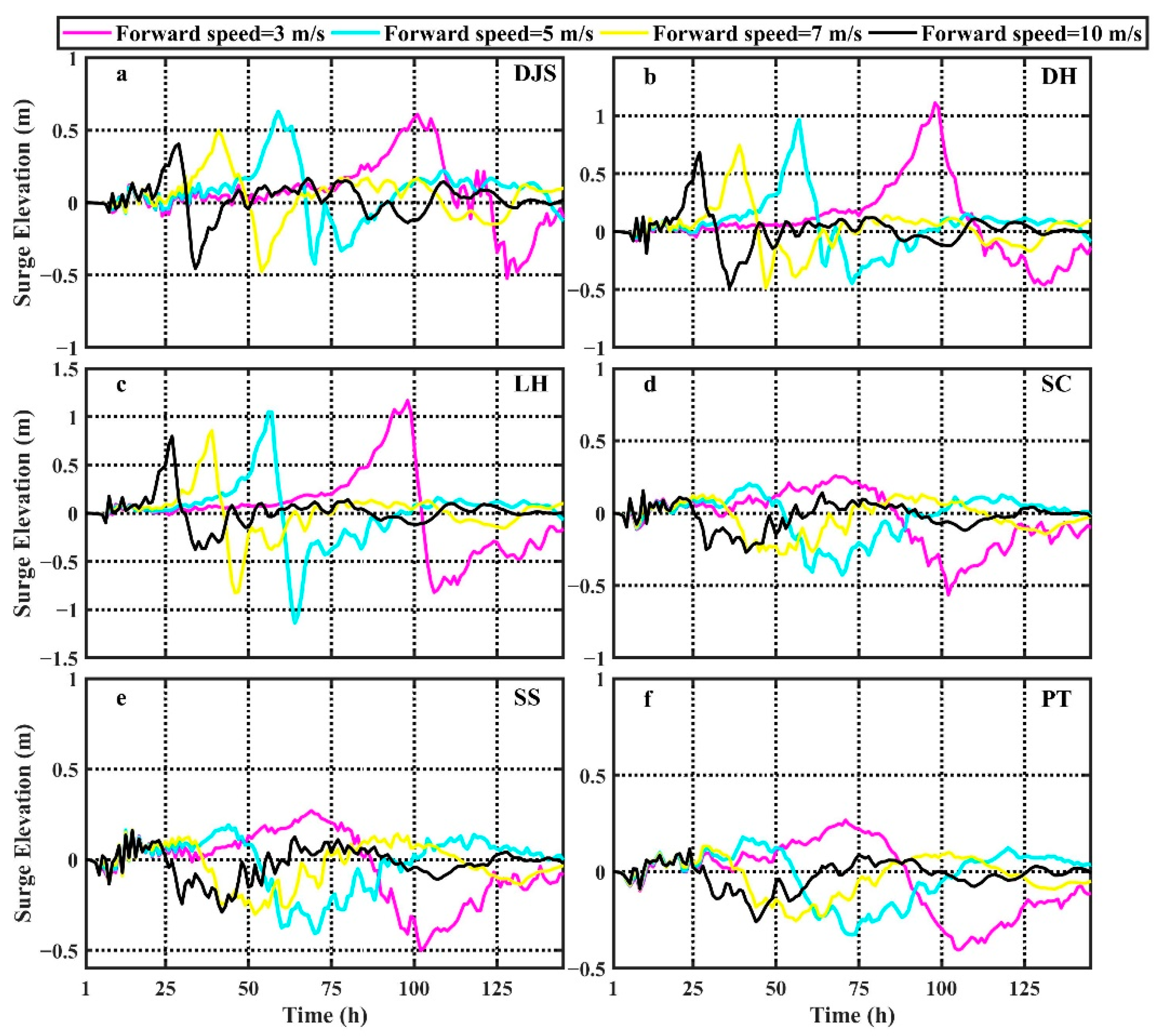
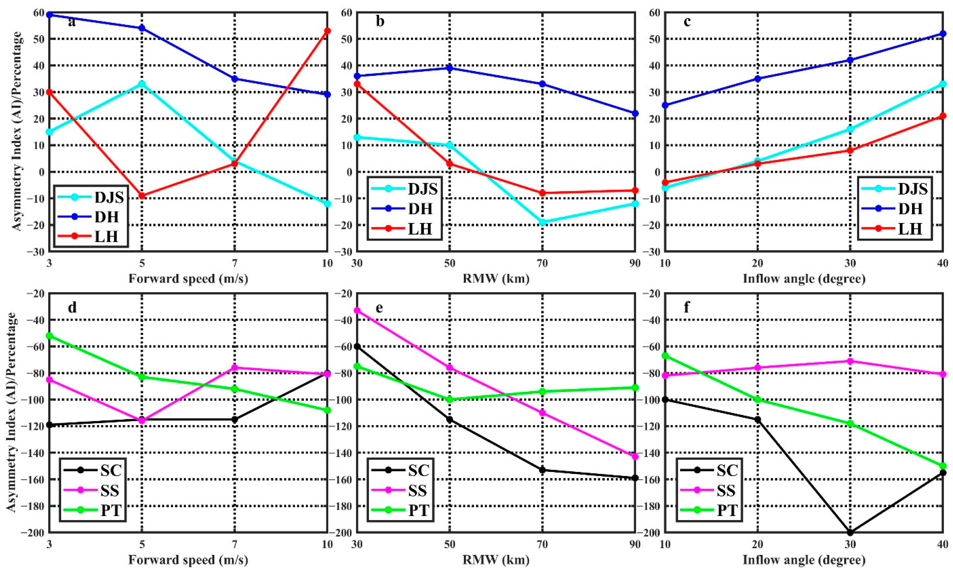
4.1.1. Effect of Forward Speed

The time series of surge elevation in different forward speed experiments at six stations are shown in Figure 5. Overall, a smaller forward speed could lead to a higher peak surge elevation, and a longer occurrence time of surge reaches the peak (from a cold start) as well as a longer duration time of high water in surge elevation. For instance, at LH station, peak surges are 1.17, 1.05, 0.86, and 0.80 m in 3, 5, 7, and 10 m/s, respectively. Besides, the occurrence time of surges reaches the peak are 98, 56, 39, 27 h, respectively, (Cases 1.1–1.4 in

Table 3. The model results of surge, fall, time, and the value of AI at the six stations. Surge (m): Surge_max; fall (m): Fall_max; time: occurrence time of surge reaches the peak (from a cold start); AI: asymmetry index.

Case Name	DJS				DH				LH
	Surge (m)	Fall (m)	Time (h)	AI (%)	Surge (m)	Fall (m)	Time (h)	AI (%)	Surge (m)	Fall (m)	Time (h)	AI (%)
1.1	0.61	−0.52	101	15	1.11	−0.46	98	59	1.17	−0.82	98	30
1.2	0.63	−0.42	59	33	0.97	−0.45	57	54	1.05	−1.14	56	−9
1.3	0.50	−0.48	41	4	0.75	−0.49	39	35	0.86	−0.83	39	3
1.4	0.41	−0.46	29	−12	0.68	−0.48	27	29	0.80	−0.38	29	53
2.1	0.30	−0.26	42	13	0.44	−0.28	39	36	0.55	−0.37	39	33
2.2	0.50	−0.45	41	10	0.75	−0.46	39	39	0.86	−0.83	39	3
2.3	0.64	−0.76	41	−19	0.94	−0.63	39	33	1.04	−1.12	39	−8
2.4	0.78	−0.87	40	−12	1.09	−0.85	39	22	1.14	−1.22	39	−7
3.1	0.47	−0.50	41	−6	0.71	−0.53	39	25	0.84	−0.87	38	−4
3.2	0.50	−0.48	41	4	0.75	−0.49	39	35	0.86	−0.83	39	3
3.3	0.51	−0.43	41	16	0.76	−0.44	39	42	0. 86	−0.79	39	8
3.4	0.52	−0.35	41	33	0.77	−0.37	39	52	0.85	−0.67	39	21
4.1	0.84	−0.79	41	6	1.26	−0.73	39	42	1.39	−1.47	39	−6
4.2	0.74	−0.64	41	14	1.08	−0.62	39	43	1.21	−1.21	39	0
4.3	0.62	−0.52	41	16	0.92	−0.55	39	40	1.03	−1.05	39	−2
4.4	0.50	−0.48	41	4	0.75	−0.49	39	35	0.86	−0.83	39	3
4.5	0.38	−0.37	41	3	0.58	−0.41	39	29	0.68	−0.66	39	3
4.6	0.27	−0.26	41	4	0.43	−0.30	39	30	0.52	−0.44	39	15
Case Name	SC				SS				PT
	Surge (m)	Fall (m)	Time (h)	AI (%)	Surge (m)	Fall (m)	Time (h)	AI (%)	Surge (m)	Fall (m)	Time (h)	AI (%)
1.1	0.26	−0.57	68	−119	0.27	−0.50	69	−85	0.27	−0.41	71	−52
1.2	0.20	−0.43	42	−115	0.19	−0.41	44	−116	0.18	−0.33	40	−83
1.3	0.13	−0.28	31	−115	0.17	−0.30	27	−76	0.13	−0.25	29	−92
1.4	0.15	−0.27	10	−80	0.16	−0.29	15	−81	0.12	−0.25	24	−108
2.1	0.10	−0.16	86	−60	0.12	−0.16	15	−33	0.08	−0.14	30	−75
2.2	0.13	−0.28	86	−115	0.17	−0.30	15	−76	0.13	−0.26	29	−100
2.3	0.17	−0.43	28	−153	0.20	−0.42	15	−110	0.18	−0.35	29	−94
2.4	0.22	−0.57	28	−159	0.23	−0.56	15	−143	0.23	−0.44	29	−91
3.1	0.15	−0.30	28	−100	0.17	−0.31	15	−82	0.15	−0.25	29	−67
3.2	0.13	−0.28	28	−115	0.17	−0.30	15	−76	0.13	−0.26	29	−100
3.3	0.10	−0.30	25	−200	0.17	−0.29	15	−71	0.11	−0.24	29	−118
3.4	0.11	−0.28	28	−155	0.16	−0.29	15	−81	0.10	−0.25	29	−150
4.1	0.20	−0.51	28	−155	0.23	−0.54	15	−135	0.21	−0.41	29	−95
4.2	0.17	−0.44	28	−159	0.21	−0.44	15	−110	0.19	−0.37	29	−95
4.3	0.16	−0.38	28	−138	0.19	−0.38	15	−100	0.16	−0.30	29	−88
4.4	0.13	−0.28	28	−115	0.17	−0.30	15	−76	0.13	−0.26	29	−100
4.5	0.11	−0.22	28	−100	0.14	−0.23	15	−64	0.11	−0.20	29	−82
4.6	0.09	−0.17	28	−89	0.12	−0.18	15	−50	0.09	−0.15	29	−67

). In Figure 5, it can be seen that the variation trends of time series of surge elevations are similar in the four forward speed experiments at the northern stations (DJS, DH, LH). Besides, similar variation trends of time series of surge elevations are found at the middle and southern stations (SC, SS, PT). When the forward speed increases from 3 m/s to 5 m/s, from 5 m/s to 7 m/s, or from 7 m/s to 10 m/s, the peak surges occur about 42, 18, or 11 h earlier than the occurrence time of peak surge when the forward speed is fixed to 3, 5, or 7 m/s at the northern stations, while 27, 13, or 13 h happens at the middle and southern stations in Cases 1.1–1.4 (Table 3). The finding indicates that the varying forward speed has a larger impact on the peak surge occurrence time at the northern stations than that at the middle and southern stations. Besides, varying the forward speed under low forward speeds (3 and 5 m/s) has a larger impact on the peak surge occurrence time than that under fast forward speeds (7 and 10 m/s).

It is interesting that, overall, the values of surge_max are higher than the absolute value of the values of fall_max at the northern stations, while the values of surge_max are lower than the absolute value of the values of fall_max at the middle and southern stations, indicating that the intensity of onshore winds (inducing positive surges) are stronger than that of offshore winds (inducing negative surges) at the northern stations, while offshore winds are suppressing onshore winds at the middle and southern stations. In summary, the values of AI are positive at the northern stations, and the values of AI are negative at the middle and southern stations. Furthermore, the relationship between the forward speed and AI varies in different stations, which is shown in Figure 6a,d. In low forward speed cases (Cases 1.1–1.2), the absolute values of AI are larger than those in fast forward speed cases (Cases 1.3–1.4) at DJS, DH, SC, and SS stations, which indicates that a lower forward speed could lead to a higher surge asymmetry at the above four stations. For example, at DH station, the values of AI are 59% and 54% in the forward speed with 3 m/s and 5 m/s, while in forward speed with 7 m/s and 10 m/s, the values of AI are 35% and 29% (Table 3).

A mechanism was proposed by Peng et al. [24] to explain the surge asymmetry response to the symmetric wind field in a 1D asymmetry, in which the pressure gradient force required to balance the wind stress is proportional to (h + ξ)dξ/dx (where h, ξ, and x are the undisturbed water depth, sea surface elevation, and distance from the coast, respectively). As indicated by the 1D asymmetry, a larger negative surge is required during fall than the corresponding positive surge. However, the horizontal surge features at the northern stations in the paper cannot be accounted by the 1D asymmetry mechanism. Possible reasons may be due to that (1) the wind field is an asymmetric wind field with the consideration of inflow angle, which produces a larger onshore wind on the northern stations than that of offshore wind, and (2) the model used in the paper considered the Coriolis force, bottom friction, and other nonlinear terms in the momentum equations; these nonlinear items play a role in positive surges and negative surges, while ignored in the assumption of 1D asymmetry mechanism.

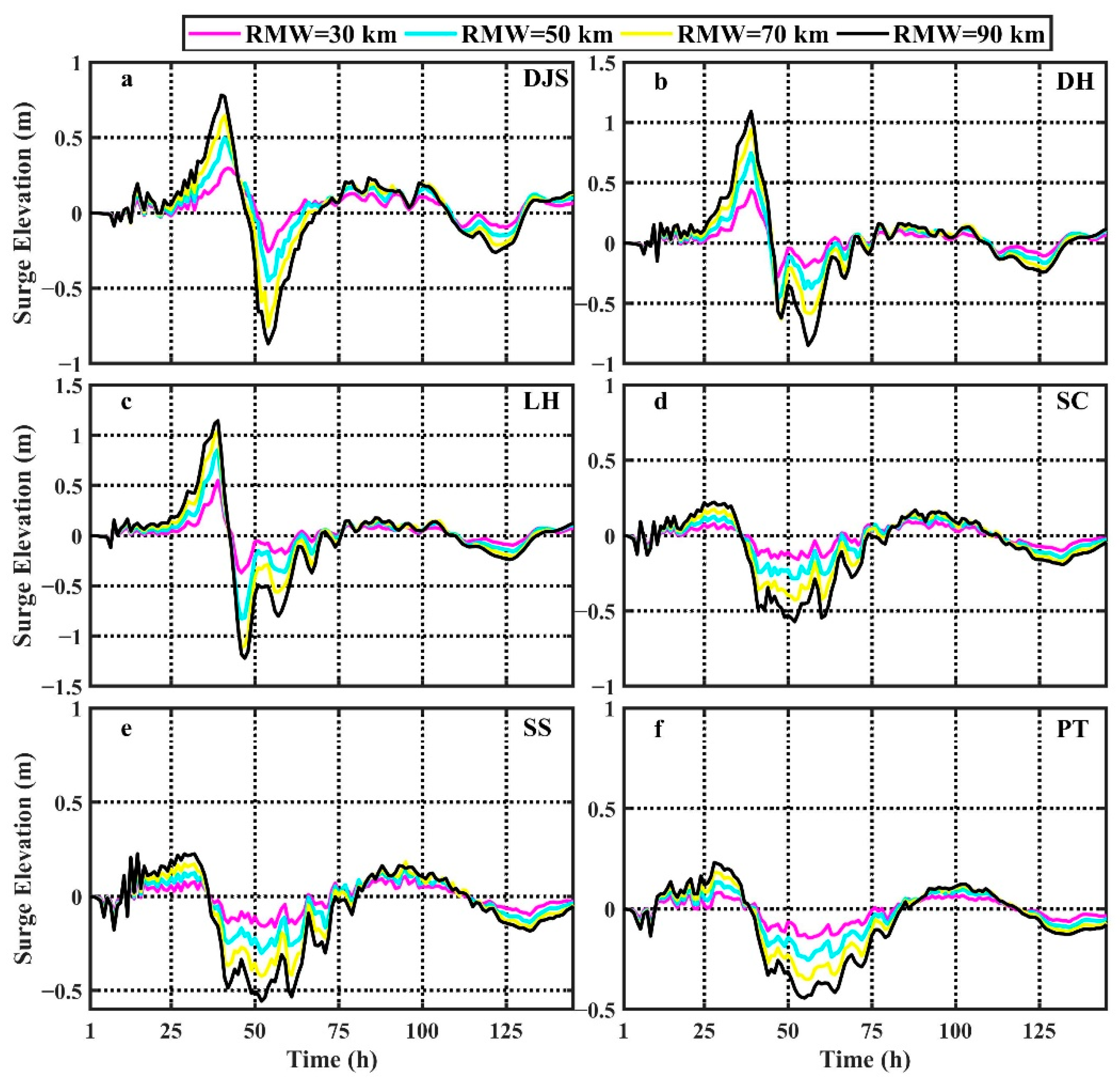
4.1.2. Effect of RMW

RMW is another parameter that plays an important role in storm surges. Unlike the effect of the forward speed (influencing the wind duration only), RMW influences not only the wind duration but also the wind fetch. Figure 7 shows the time series of surge elevation in different RMW experiments at the six stations. It can be seen that a larger RMW produces higher Surge_max and Fall_max simultaneously at the six stations. Besides, the peak surge occurrence time occurs earlier with a larger RMW, but within 2 h difference at DJS, DH, LH, SS, and PT stations (Cases 2.1–2.4 in Table 3). For example, the values of Surge_max are 0.55, 0.86, 1.04, 1.14 m, and the values of Fall_max are −0.37, −0.83, −1.12, −1.22 m at LH station in Cases 2.1–2.4. Besides, the occurrence time of peak surge is 39 h in four cases at LH station. Meanwhile, the Surge_max (or Fall_max) increases (or decrease) significantly when RMW increases from 30 km (Case 2.1) to 50 km (Case 2.2), with an average increase of 55% (or a decrease of 85%) in comparison with the Surge_max (or Fall_max) in Case 2.1 at the six stations. However, when RMW increases from 70 km (Case 2.3) to 90 km (Case 2.4), the Surge_max (or Fall_max) increases (or decreases) much smaller than those when RMW increases from 30 to 50 km, which can be inferred from Figure 7. Furthermore, a larger RMW could lead to a lower value of AI (Figure 6b,e). For example, the values of AI are 33%, 3%, −8%, and −7% at LH station in Cases 2.1–2.4. It is noted that the values of AI decrease with an increase of RMW at SC, SS, and PT stations in Cases 2.1–2.4; however, the values of AI are negative at these stations, and a lower negative value of AI represents a stronger asymmetry between Surge_max and Fall_max, which indicates that a larger RMW leads to a stronger surge asymmetry at these three stations.

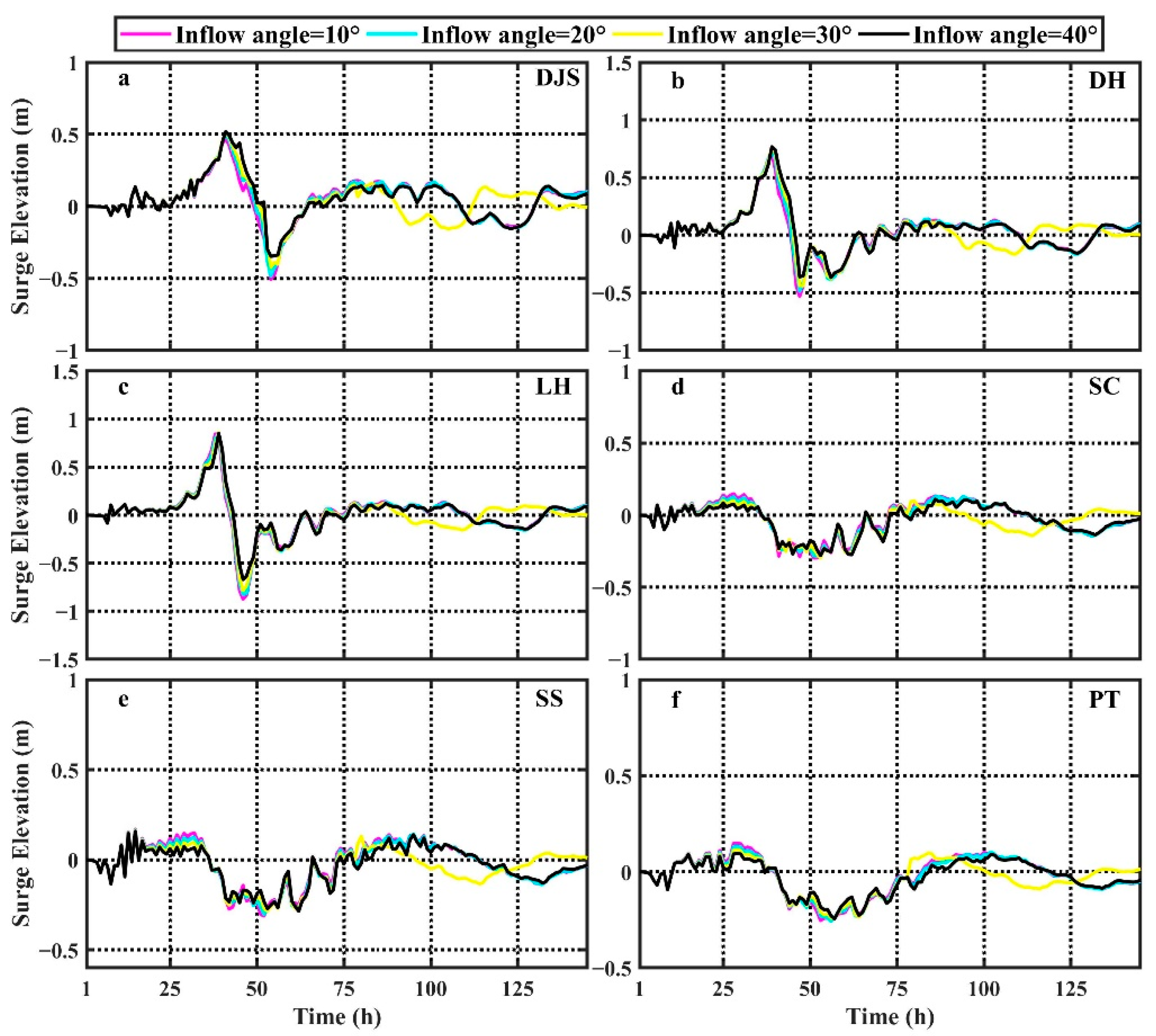
4.1.3. Effect of Inflow Angle

The inflow angle can change the asymmetry of the wind field and the direction of tropical cyclones, which may influence the positive surges and the negative surges. As shown in Figure 8, there is no apparent difference in Surge_max when modifying the inflow angle in the wind field at the northern stations (DJS, DH, and LH station), which indicates that a steady state for positive surges was reached at some time at these three stations. However, the Fall_max decreases when increasing the inflow angle, which shows that a larger inflow angle leads to a stronger surge asymmetry between Surge_max and Fall_max, which can be inferred from Figure 6c,f. For example, the values of Surge_max are 0.84, 0.86, 0.86, and 0.85 m, and the values of Fall_max are −0.87, −0.83, −0.79, and −0.67 m at LH station when the inflow angle increases from 10° to 40° (Cases 3.1–3.4 in Table 3), which leads to an increase of AI from −4% to 21%.

The reason why the inflow angle can change the surge asymmetry mainly attributes to the asymmetry of wind filed and the orientation of the typhoon path [24]. A typhoon moving northward with land on its left in the Northern Hemisphere may cause a higher value of Surge_max with the consideration of inflow angle in the wind field, which is consistent with the result in the paper.

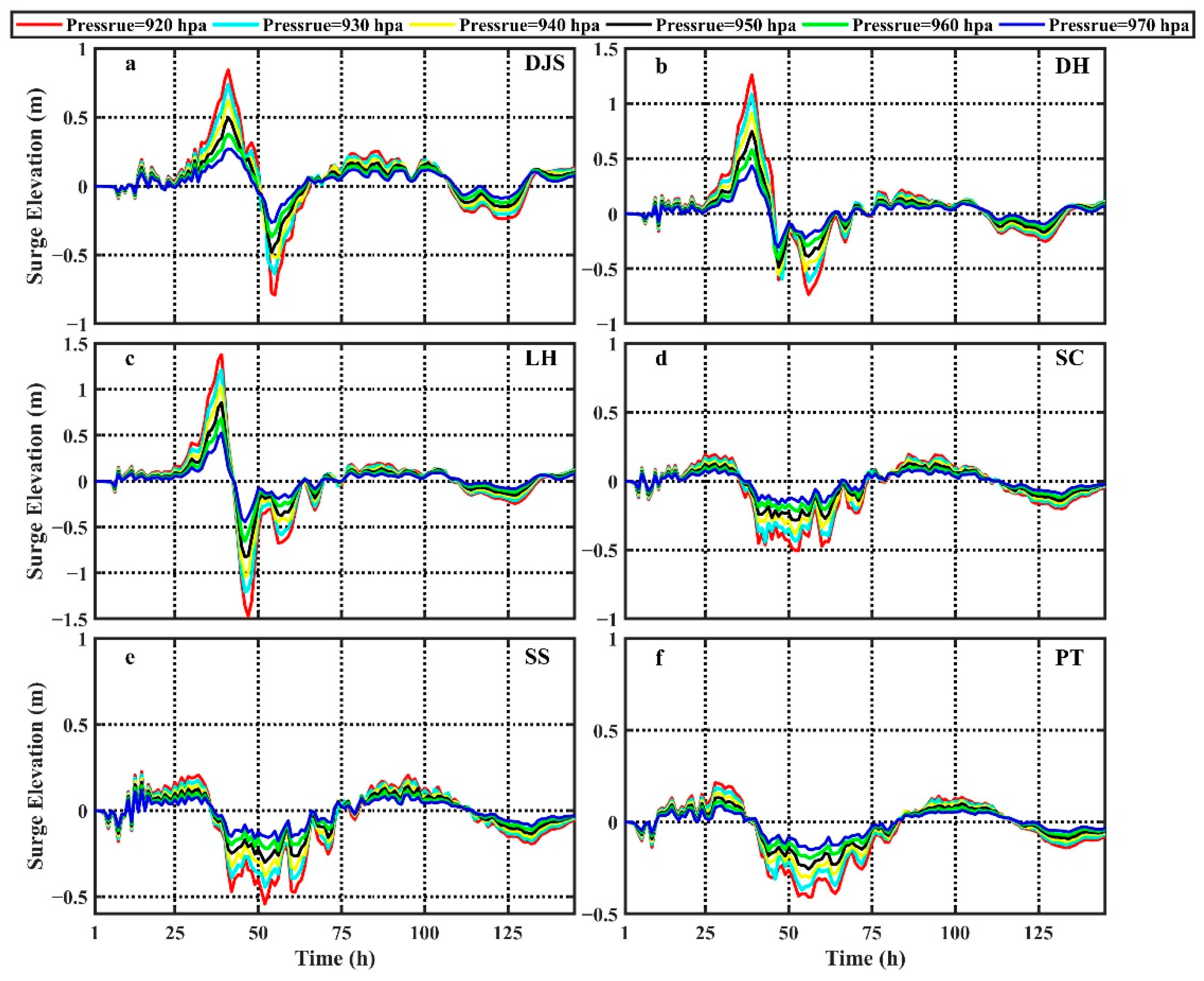
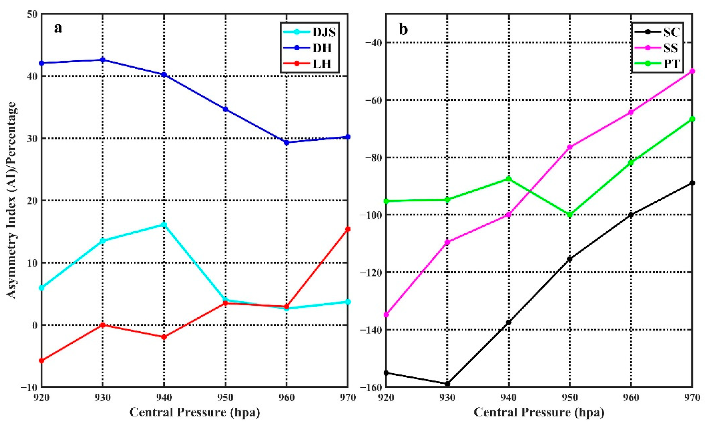
4.1.4. Effect of Central Pressure

Figure 9 shows the time series of surge elevations in different central pressure experiments at the six stations. It can be seen that a lower central pressure produces a higher Surge_max and Fall_max simultaneously in Cases 4.1–4.6, which shows a similar function as increasing RMW in the surge elevation. Besides, a lower central pressure leads to a longer duration time of high water in the surge elevation. However, changing central pressure does not affect the peak surge occurrence time in the sensitivity experiments (Cases 4.1–4.6 in Table 3). Overall, a smaller central pressure leads to a stronger surge asymmetry, even though the values of Surge_max and Fall_max are relatively smaller at LH, SC, SS, and PT stations, which can be inferred from Table 3 and Figure 10. For instance, the value of AI increases from −135% to −50% when the central pressure increases from 920 to 970 hPa at SS station.

Besides, sensitivity experiments of other factors that influence storm surges are conducted. The factors include typhoon path, the intensity of wind field, and topography. The path experiments are varied in different typhoon cases. Wind intensity experiments are varied from 50% of default wind intensity (low wind intensity) to 120% of default wind intensity (strong wind intensity).

Table 4. Settings of sensitivity experiments to explore the effects of typhoon path, wind intensity, and topography on storm surges.

Case Name	Path	Wind Intensity	Bathymetry
5.1	Chan-hom	100%	Default bathymetry (h)
5.2	Chan-hom	50%	h
5.3	Chan-hom	120%	h
5.4	Chan-hom	100%	h × 0.25
5.5	Chan-hom	100%	h × 0.5
5.6	Chan-hom	100%	h × 0.75
6.1	Mireille	100%	h
6.2	Mireille	50%	h
6.3	Mireille	120%	h
6.4	Mireille	100%	h × 0.25
6.5	Mireille	100%	h × 0.5
6.6	Mireille	100%	h × 0.75
7.1	Herb	100%	h
7.2	Herb	50%	h
7.3	Herb	120%	h
7.4	Herb	100%	h × 0.25
7.5	Herb	100%	h × 0.5
7.6	Herb	100%	h × 0.75
8.1	Winnie	100%	h
8.2	Winnie	50%	h
8.3	Winnie	120%	h
8.4	Winnie	100%	h × 0.25
8.5	Winnie	100%	h × 0.5
8.6	Winnie	100%	h × 0.75

shows the details of sensitivity experiments of typhoon path, wind intensity, and topography on storm surge simulations. To evaluate the effects of these factors on storm surges, some parameters in the wind and pressure field should be fixed. In this section, the forward speed is fixed to 7 m/s. RMW, inflow angle, and central pressure are set to 50 km, 20°, and 950 hPa, respectively. The bathymetry in Section 4.2 and Section 4.3 used water depth in Section 3.1.

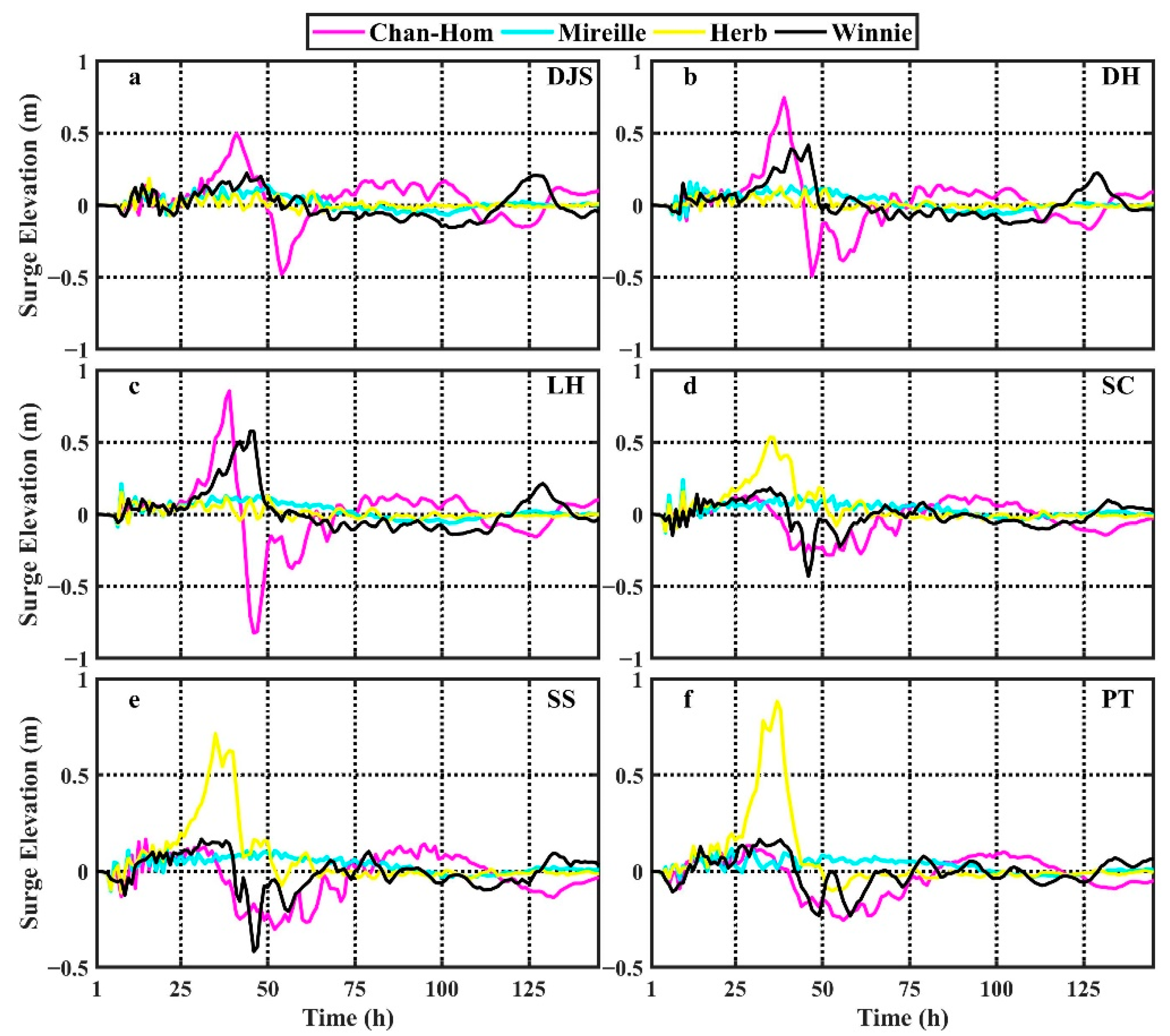
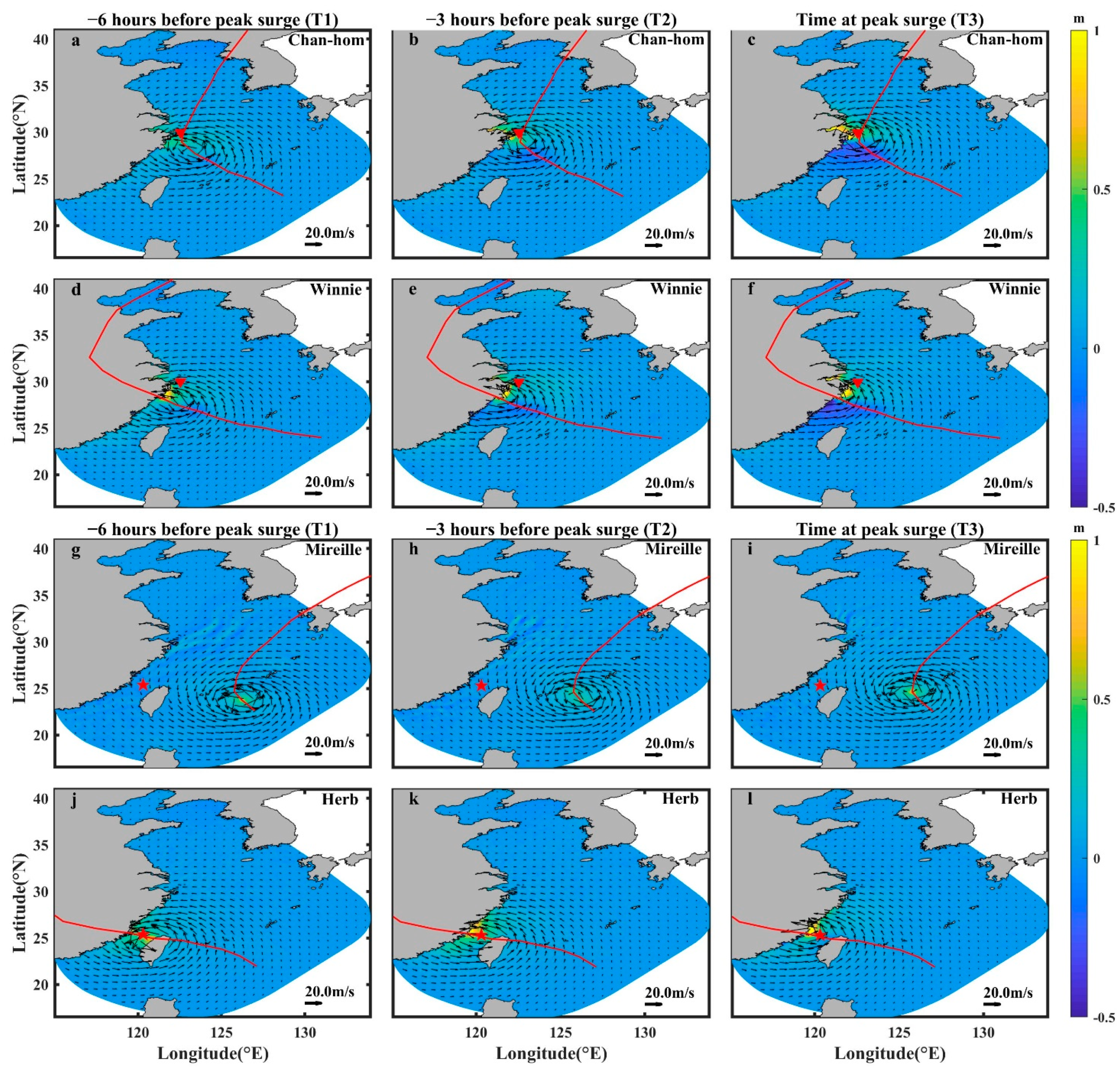
4.2. Effect of Typhoon Path

Figure 11 shows the time series of surge elevations at the six locations during the four typhoon path simulations. The surge elevation forced with the path of Chan-hom (Case 5.1) is the highest followed by Winnie (Case 8.1), Herb (Case 7.1), and Mireille (Case 6.1) at DJS, DH, and LH stations (Figure 11a–c). Besides, the earliest occurrence time of peak surge was Chan-hom, and Winnie was delayed for a few hours. In SC, SS, and PT stations (Figure 11d–f), the path of Herb induced the highest surge elevation. The paths of Chan-hom and Winnie are relatively comparable, and the path of Mireille is the lowest. This is mainly due to the paths of Chan-hom and Winnie are near the DJS, DH, and LH stations, while those of Herb and Mireille are relatively far away, beyond their maximum radius. Likewise, the path of Herb was the nearest to the SC, SS, and PT stations, which induced the highest surge elevations in these three stations.

Comparing the peak surge elevation at each station during the paths of Chan-hom and Winnie, it can be found that peak surge elevations induced by Chan-hom (type 1) are higher than those induced by Winnie (type 4) at DJS, DH, and LH stations, which indicates that the typhoon paths, such as Chan-hom (type 1), can generate storm surges more easily than those paths, such as Winnie’s (type 4) in Zhoushan Archipelago (Figure 2a). For path Herb (type 3), it has a big influence at PT station and has minor impacts at DJS, DH, and LH stations. For path Mireille (type 2), the surge elevations at the six stations are small, which implies that this type of typhoon path has a minor impact on surge elevation along the SCC.

As the surge elevation was caused by wind stress and pressure gradient, to be more specific, three groups of these four paths experiments were conducted. In group one, the surge models were forced by the wind field and pressure field. In group two, the models were driven by the wind field only. In group three, the models were forced by the pressure field only.

Three groups of surge elevation at the six stations during the four paths are shown in

Table 5. The model results of peak surges in group one, group two, and group three at each station during with four paths.

Path	Station	Group One	Group Two	Group Three	Group Two + Group Three
Chan-hom	DJS	0.50	0.40	0.12	0.52
	DH	0.75	0.61	0.15	0.76
	LH	0.86	0.66	0.22	0.88
	SC	0.13	0.14	0.01	0.15
	SS	0.17	0.01	0.16	0.17
	PT	0.14	0.07	0.07	0.14
Mireille	DJS	0.14	0.11	0.06	0.17
	DH	0.16	0.01	0.15	0.16
	LH	0.21	0.01	0.21	0.22
	SC	0.24	0.01	0.24	0.25
	SS	0.11	0.03	0.09	0.12
	PT	0.12	0.01	0.11	0.12
Herb	DJS	0.19	0.01	0.18	0.19
	DH	0.13	0.03	0.10	0.14
	LH	0.16	0.01	0.16	0.17
	SC	0.53	0.45	0.10	0.55
	SS	0.72	0.60	0.14	0.74
	PT	0.88	0.45	0.44	0.89
Winnie	DJS	0.22	0.15	0.07	0.22
	DH	0.42	0.29	0.14	0.43
	LH	0.58	0.48	0.11	0.59
	SC	0.18	0.13	0.04	0.17
	SS	0.17	0.11	0.06	0.17
	PT	0.17	0.10	0.07	0.17

. It can be found that during the path Chan-hom and Winnie, the surge elevations are mainly induced by the wind field, and pressure field played minor role in surge elevations. Besides, the surge elevations forced by the pressure for path Chan-hom are larger than those for path Winnie at DJS, DH, and LH stations. It is due to that the pressure field for path Chan-hom is smaller than that for path Winnie at these three stations. For path Herb, the effect of pressure field is the major forcing for the surge elevation at the three stations (DJS, DH, LH), while at SC and SS stations, the wind field plays a dominant role in the peak surge elevation. At PT station, compared to the pressure field, the wind field plays a comparable role in the surge elevation. For path Mireille, the pressure field plays a significant role in surge elevation, and the surge elevation is mostly attributed to the pressure field at the six stations.

As shown in Table 5, the surge elevation caused by the wind field plus pressure field is larger than that of wind plus pressure field together, which indicates that a non-linear effect exists between wind field and pressure field on the surge elevation, and the nonlinear interaction between the wind field and wind pressure filed tends to weaken the surge elevation.

Furthermore, the wind field and pressure field from the model results at three selected time periods are plotted for analysis (Figure 12 and Figure 13). Three-time nodes are selected as 6 h before the peak surge arrived (T1), 3 h before the peak surge arrived (T2), and the time of peak surge arrived (T3). For simplicity, LH and PT stations are chosen to represent the north station and the south station for analysis, respectively.

For path Chan-hom (Figure 12a–c), the wind direction is approximately northwest at time T1 and then turn into northeast at time T3 while passing through LH station. Such a wind direction could blow seawater from the open sea to the Zhoushan Archipelago and then transport it to the Hangzhou Bay. Due to the unique mouth geometry of the Hangzhou Bay, the transported seawater will accumulate here, which leads to the high sea surface elevation. For path Winnie (Figure 12d–f), the wind direction is northwest at time T1, T2, and T3 when passing through LH station, and such wind field could blow seawater from the open sea to the Zhoushan Archipelago and lead to a high sea surface elevation. However, LH station is located out of the range of the maximum radius of the wind field. The wind speed of path Winnie is relatively smaller than that of path Chan-hom at time T3, which explains why the peak surge induced by path Chan-hom is higher than that induced by path Winnie. For path Mireille (Figure 12g–i), the center of the wind field is beyond east of 125° E, and the wind speed is very small along the SCC. Hence, the wind stress has a minor effect on the sea level variation. For path Herb (Figure 12j–l), because the PT station is located within the scope of maximum radius of wind field of Herb, the peak surge at PT is the highest among the six stations.

In general, the variation of surge elevation forced by the pressure field could be attributed to that the inverse barometer effect [49,50]. The surface pressure fields are plotted in Figure 13 at the time of T1, T2, and T3. The pressure field has an impact on the surge elevation in the vicinity of the pressure field center. Overall, 1 hPa of pressure drop leads to 1 cm sea surface elevation rise in the case in which seawater can freely flow to the low-pressure areas. As the wind field and the pressure field are coupled in Equations (14)–(17), a changed pressure is expected to influence the wind field. In the study of Musinguzi and Akbar [22], a 30 hPa pressure drop results in a 0.2 m increasing of the surge elevation. However, a 37.3 hPa pressure drop results in a 0.73 m increasing of the surge elevation in the model results of Feng et al. [20]. In this paper, at LH station for example, a 22.0 hPa (Chan-hom), a 4.0 hPa (Mireille), a 3.6 hPa (Herb), and a 13.6 hPa (Winnie) pressure drop at time T3 during four paths simulations, respectively. Besides, the pressure field contributes 0.22, 0.21, 0.16, and 0.11 m to the surge elevation in the above four paths simulations (Table 5). As a result, a 22.0 hPa pressure drop leads to a 0.22 m increasing of sea level for path Chan-hom, which could be explained by the inverse barometer effect. In addition, a 4.0 hPa and a 3.6 hPa pressure drop result in a 0.21 m and a 0.16 m increasing of sea level for path Mireille and Herb, respectively. It may be due to that horizontal convergence of the water and surge wave reflection against the coastline, which leads to an increase of inverse barometer effect [20]. However, a 13.6 hPa pressure drop leads to a 0.11 m increasing of sea level for path Winnie, and it may be due to that seawater cannot freely flow to the low-pressure areas during the Winnie passing through, which is limited by the coastline as shown in Figure 13f.

As the RMW is fixed to 50 km in the sensitivity experiments in Table 4, the four paths (Chan-hom, Mireille, Herb, and Winnie) are too far away from each other. For a more comprehensive understanding of the path’s impact on storm surges, it is better to conduct sensitivity experiments under one type of typhoon path. In this part, eight hypothetical path sensitivity experiments, based on the path of Chan-hom, are conducted to study the effect of different path on the modeling of storm surges. The eight hypothetical paths are shown in Figure 14, which is moved left (or right) 0.5°, 1°, 1.5°, and 2° in the longitude direction, respectively. The details of sensitivity experiments are shown in

Table 6. Sensitivity experiments to explore the effect of typhoon path on storm surges.

Case Name	Path	Remark
9.0	default (Chan-hom)	Ori
9.1	move rightward 2° in longitude direction	lon + 2
9.2	move rightward 1.5° in longitude direction	lon + 1.5
9.3	move rightward 1° in longitude direction	lon + 1
9.4	move rightward 0.5° in longitude direction	lon + 0.5
9.5	move leftward 0.5° in longitude direction	Lon − 0.5
9.6	move leftward 1° in longitude direction	Lon − 1
9.7	move leftward 1.5° in longitude direction	Lon − 1.5
9.8	move leftward 2° in longitude direction	Lon − 2

.

The time series of surge elevations at six stations in hypothetical paths are shown in Figure 15. Overall, when moving right (Cases 9.1–9.4), the surge elevations are lower than the values in the default path at six stations, which indicates that a farther path moved rightward leads to a lower surge elevation (Cases 9.1–9.4 in

Table 7. The model results of surge, fall, time, and the value of AI in different paths at six stations. Surge (m): Surge_max; fall (m): Fall_max; time: occurrence time of surge reaches the peak (from a cold start); AI: asymmetry index.

Case Name	DJS				DH				LH
	Surge (m)	Fall (m)	Time (h)	AI (%)	Surge (m)	Fall (m)	Time (h)	AI (%)	Surge (m)	Fall (m)	Time (h)	AI (%)
9.0	0.50	−0.48	41	4	0.75	−0.49	39	35	0.86	−0.82	39	5
9.1	0.26	−0.29	71	−12	0.26	−0.24	40	8	0.25	−0.24	40	4
9.2	0.29	−0.28	71	3	0.33	−0.23	40	30	0.31	−0.24	40	23
9.3	0.27	−0.28	78	−4	0.37	−0.24	40	35	0.31	−0.22	40	29
9.4	0.35	−0.24	41	31	0.47	−0.21	39	55	0.50	−0.29	39	42
9.5	0.65	−0.96	41	−48	1.06	−0.75	39	29	1.29	−1.07	38	17
9.6	0.86	−1.03	45	−20	0.96	−0.83	39	14	1.34	−0.81	39	40
9.7	0.66	−1.94	45	−194	0.44	−0.79	48	−80	0.75	−0.82	39	−9
9.8	0.40	−1.53	106	−283	0.34	−0.63	108	−85	0.39	−0.66	35	−69
Case Name	SC				SS				PT
	Surge (m)	Fall (m)	Time (h)	AI (%)	Surge (m)	Fall (m)	Time (h)	AI (%)	Surge (m)	Fall (m)	Time (h)	AI (%)
9.0	0.13	−0.28	94	−115	0.17	−0.30	15	−76	0.13	−0.26	29	−100
9.1	0.11	−0.19	14	−73	0.10	−0.20	14	−100	0.11	−0.16	15	−45
9.2	0.11	−0.24	14	−118	0.12	−0.25	17	−108	0.12	−0.19	15	−58
9.3	0.14	−0.27	88	−93	0.15	−0.26	13	−73	0.11	−0.21	15	−91
9.4	0.17	−0.29	88	−71	0.16	−0.27	15	−69	0.11	−0.25	28	−127
9.5	0.15	−0.39	28	−160	0.15	−0.38	15	−153	0.16	−0.26	29	−63
9.6	0.19	−0.44	10	−132	0.16	−0.39	25	−144	0.18	−0.28	29	−56
9.7	0.25	−0.34	10	−36	0.20	−0.35	25	−75	0.19	−0.27	28	−42
9.8	0.29	−0.31	10	−7	0.26	−0.29	27	−12	0.21	−0.20	24	5

). On the contrary, when moving left (Cases 9.5–9.6), the values of Surge_max are larger than the values in the default path at DJS, DH, and LH stations. Moreover, with the decrease of the latitude of six stations, moving left (Cases 9.7–9.8) plays a significant role in the peak surge elevation. For example, when moving left 0.5°, 1°, and 1.5° (Cases 9.5–9.7), the values of Surge_max are 0.65, 0.86, and 0.66 m at DJS station (Table 7), which are higher than the value of Surge_max in the default path (0.50 m in Case 9.0). However, when moving left 2° (Case 9.8), the peak surge elevation is 0.40 m, which is lower than the value in the default path. The values of Fall_max in the above four cases are −0.96, −1.03, −1.94, and −1.53 m, respectively. The value of Fall_max in the default path is −0.48 m, which indicates that moving left, the path has a larger impact on the Fall_max than the Surge_max at DJS station. At DH and LH stations, the trends of the time series of surge elevations are similar to that at DJS station. At SC, SS, and PT stations, the values of Surge_max are lower than those at DJS, DH, and LH stations, which indicate that the path of Chan-hom (type 1) has a larger influence on the northern stations than the southern stations along the SCC.

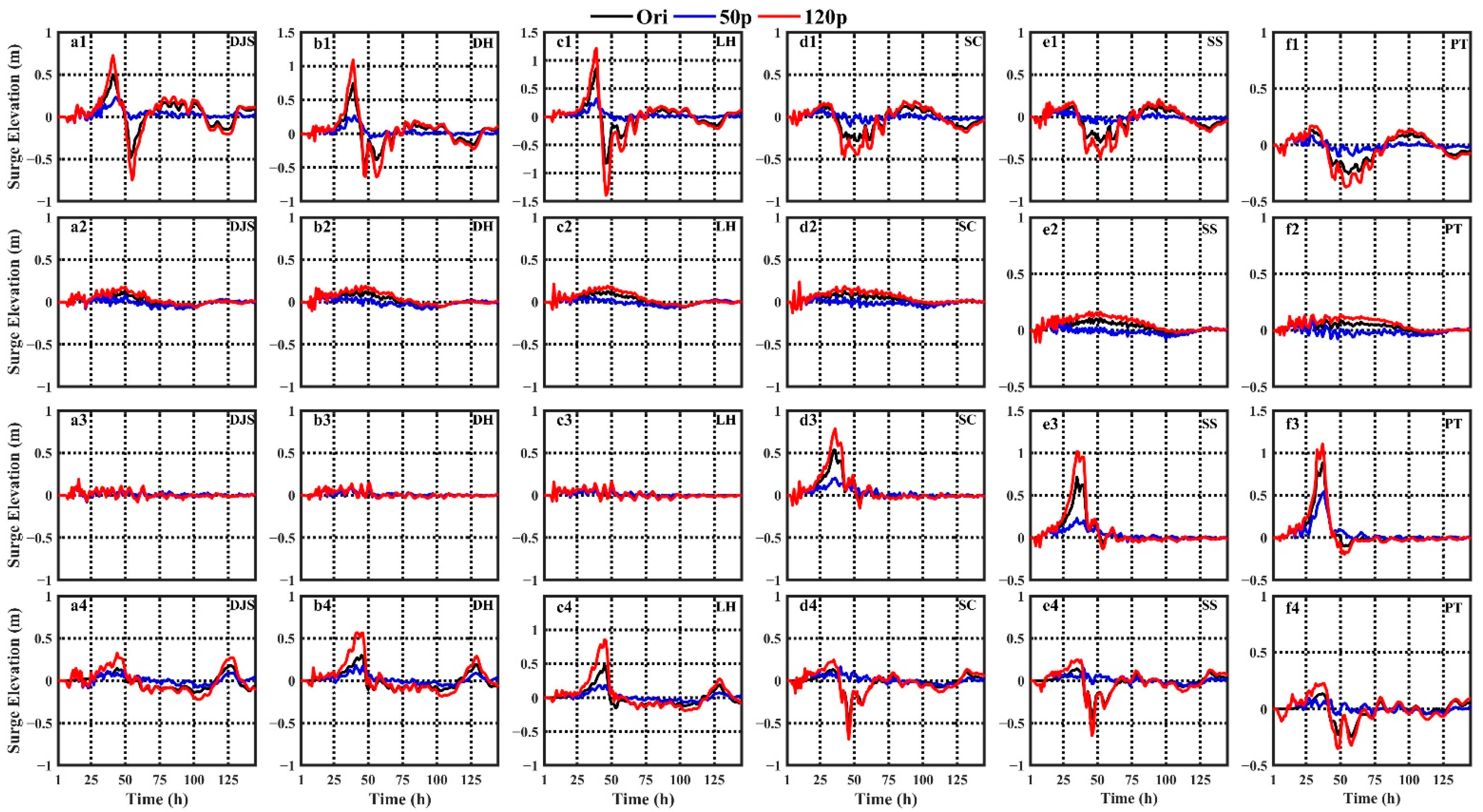
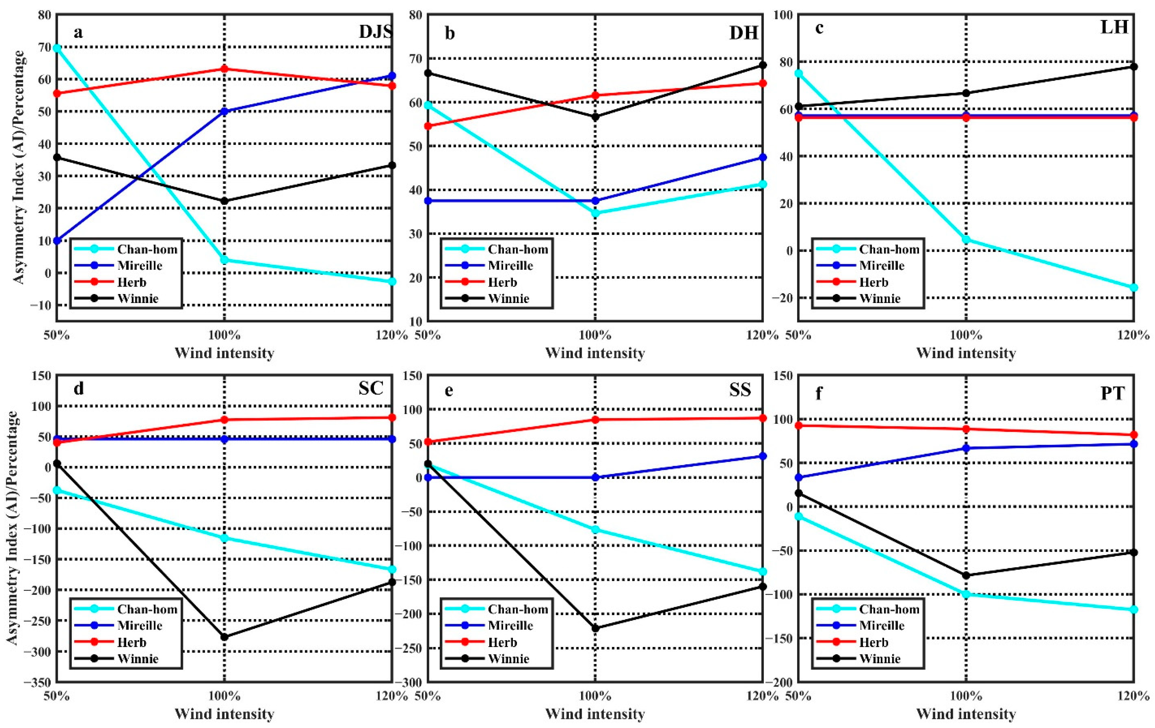
4.3. Effect of Wind Intensity

In this section, 50% of default wind intensity (low wind intensity) to 120% of default wind intensity (strong wind intensity) are conducted to evaluate the effect of wind intensity on storm surges. The details of wind intensity sensitivity experiments are shown in Table 4.

Figure 16 shows the maximum wind velocity and the maximum sea surface elevation at every mesh node over the entire modeling time in Cases 5.1–5.3 (path Chan-hom). It can be seen that surge elevations decrease with the 50% wind intensity in Figure 16d (Case 5.2) or surge elevations increase with the 20% wind intensity in Figure 16f (Case 5.3). However, it should be noticed that, as the wind intensity increases (or decreases), the size of wind field also increases (or decreases), which can be inferred from Figure 16c,e. As a result, the variation of surge elevation is a combined effect of wind intensity and size of wind field. A similar finding was reported by Irish et al. [51], in which they found that the effect of varying wind intensity on a storm surge is similar in magnitude to that of varying the RMW in the wind field.

Besides, for the impact of wind intensity, two apparent characteristics can be found in Figure 17. One is that decreasing the wind intensity has an opposite effect on surge elevations in comparison to increasing the wind intensity; however, as the wind intensity changes, the surge elevation changes with inequality proportion. The other characteristic is that changing wind intensity has a larger impact on peak surge elevation than the occurrence time of surge reaching the peak. For example, in the path of Chan-hom (Figure 17a1–c1), the values of Surge_max are 0.50, 0.75, and 0.86 m at DJS, DH, and LH station in default wind intensity experiment (Case 5.1 in

Table 8. The model results of surge, fall, time, and the value of AI in different wind intensity during four paths at six stations. Surge (m): Surge_max; fall (m): Fall_max; time: occurrence time of surge reaches the peak (from a cold start); AI: asymmetry index.

Case Name	DJS				DH				LH
	Surge (m)	Fall (m)	Time (h)	AI (%)	Surge (m)	Fall (m)	Time (h)	AI (%)	Surge (m)	Fall (m)	Time (h)	AI (%)
5.1	0.50	−0.48	41	4	0.75	−0.49	39	35	0.86	−0.82	39	5
5.2	0.23	−0.07	43	70	0.27	−0.11	40	59	0.32	−0.08	39	75
5.3	0.73	−0.75	41	−3	1.09	−0.64	39	41	1.21	−1.40	39	−16
6.1	0.14	−0.07	50	50	0.16	−0.10	12	38	0.21	−0.09	8	57
6.2	0.10	−0.09	16	10	0.16	−0.10	12	38	0.21	−0.09	8	57
6.3	0.18	−0.07	50	61	0.19	−0.10	48	47	0.21	−0.09	8	57
7.1	0.19	−0.07	16	63	0.13	−0.05	38	62	0.16	−0.07	8	56
7.2	0.18	−0.08	16	56	0.11	−0.05	38	55	0.16	−0.07	8	56
7.3	0.19	−0.08	16	58	0.14	−0.05	51	64	0.16	−0.07	50	56
8.1	0.18	−0.14	127	22	0.30	−0.13	45	57	0.48	−0.16	45	67
8.2	0.14	−0.09	14	36	0.18	−0.06	41	67	0.18	−0.07	41	61
8.3	0.33	−0.22	44	33	0.57	−0.18	42	68	0.86	−0.19	45	78
Case Name	SC				SS				PT
	Surge (m)	Fall (m)	Time (h)	AI (%)	Surge (m)	Fall (m)	Time (h)	AI (%)	Surge (m)	Fall (m)	Time (h)	AI (%)
5.1	0.13	−0.28	94	−115	0.17	−0.30	15	−76	0.13	−0.26	29	−100
5.2	0.08	−0.11	25	−38	0.16	−0.13	15	19	0.09	−0.10	15	−11
5.3	0.18	−0.48	86	−167	0.21	−0.50	95	−138	0.17	−0.37	29	−118
6.1	0.24	−0.13	10	46	0.11	−0.11	21	0	0.12	−0.04	13	67
6.2	0.24	−0.13	10	46	0.11	−0.11	10	0	0.12	−0.08	13	33
6.3	0.24	−0.13	10	46	0.16	−0.11	44	31	0.14	−0.04	30	71
7.1	0.53	−0.12	35	77	0.72	−0.11	35	85	0.88	−0.10	37	89
7.2	0.20	−0.12	36	40	0.23	−0.11	35	52	0.54	−0.04	38	93
7.3	0.79	−0.15	36	81	1.01	−0.13	35	87	1.11	−0.20	37	82
8.1	0.13	−0.49	35	−277	0.14	−0.45	35	−221	0.14	−0.25	37	−79
8.2	0.16	−0.15	40	6	0.15	−0.12	40	20	0.13	−0.11	15	15
8.3	0.24	−0.69	35	−188	0.25	−0.65	35	−160	0.23	−0.35	38	−52

). When decreasing wind intensity by 50%, the values of Surge_max (or the ratio change compared with Case 5.1) are 0.23 (−54%), 0.27 (−64%), and 0.32 m (−63%) at the above three stations (Case 5.2 in Table 8). The values of Surge_max (or the ratio changes compared with Case 5.1) are 0.73 (+46%), 1.09 (+45%), and 1.21 m (+41%) when increasing wind intensity by 20% (Case 5.3 in Table 8). In addition, the occurrence time of surge reaching the peak is almost the same at these three stations. Similar results are also found in the model results in path Mireille (Figure 17a2–f2), path Herb (Figure 17a3–f3), and path Winnie (Figure 17a4–f4).

The relationship between AI and wind intensity during four path simulations varies in path type, which is shown in Figure 18. For path Chan-hom (Cases 5.1–5.3), overall, the values of AI decrease with the increase of wind intensity at six stations. The values of AI are positive at DJS, DH, and LH stations, while the values of AI are negative at SC, SS, and PT stations. A lower negative value of AI represents a stronger asymmetry between Surge_max and Fall_max, which can be inferred from Figure 17d1–f1. For path Mireille (Cases 6.1–6.3), the surge asymmetry increases with the increase of wind intensity. For path Herb (Cases 7.1–7.3), a stronger wind field could lead to a strengthening of surge asymmetry at DH, LH, SC, and SS stations. For path Winnie (Cases 8.1–8.3), the relationship between surge asymmetry and wind intensity is heterogeneous and varies with the stations.

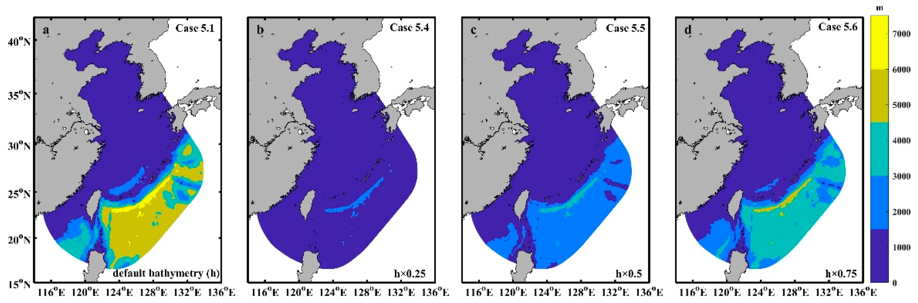
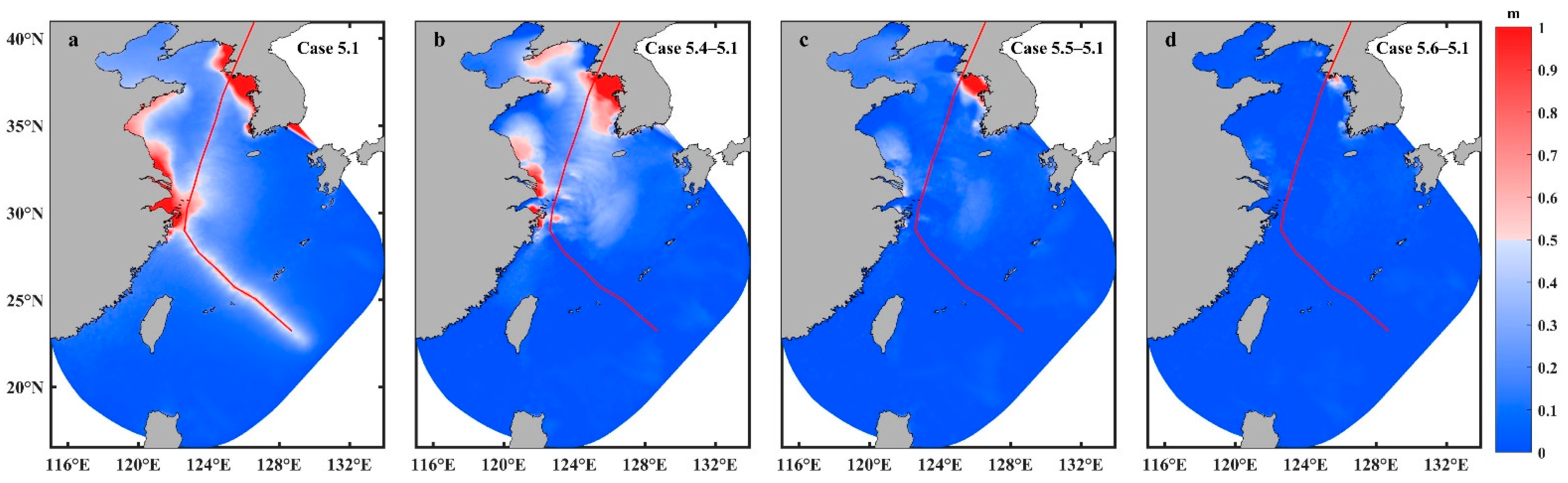
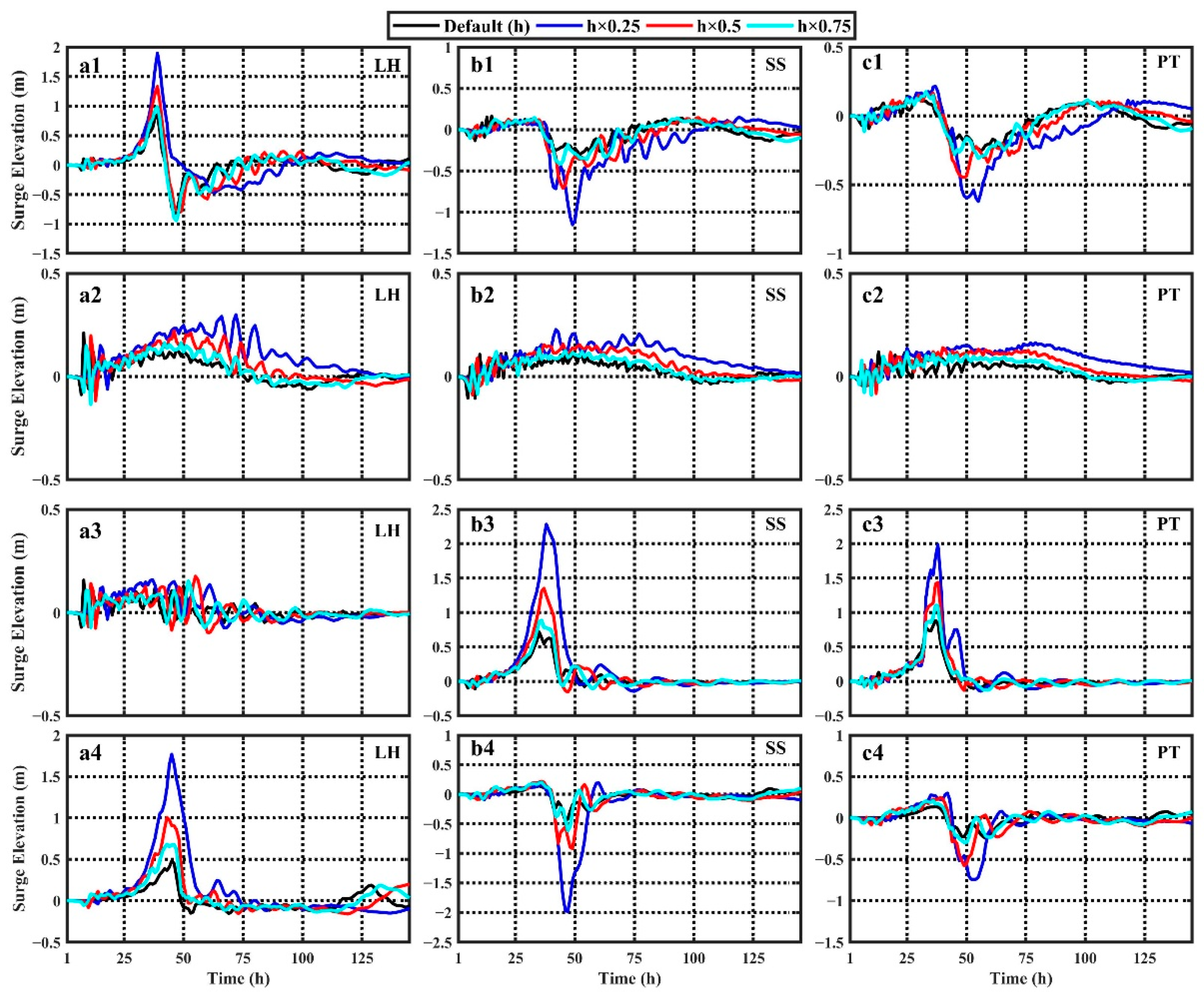
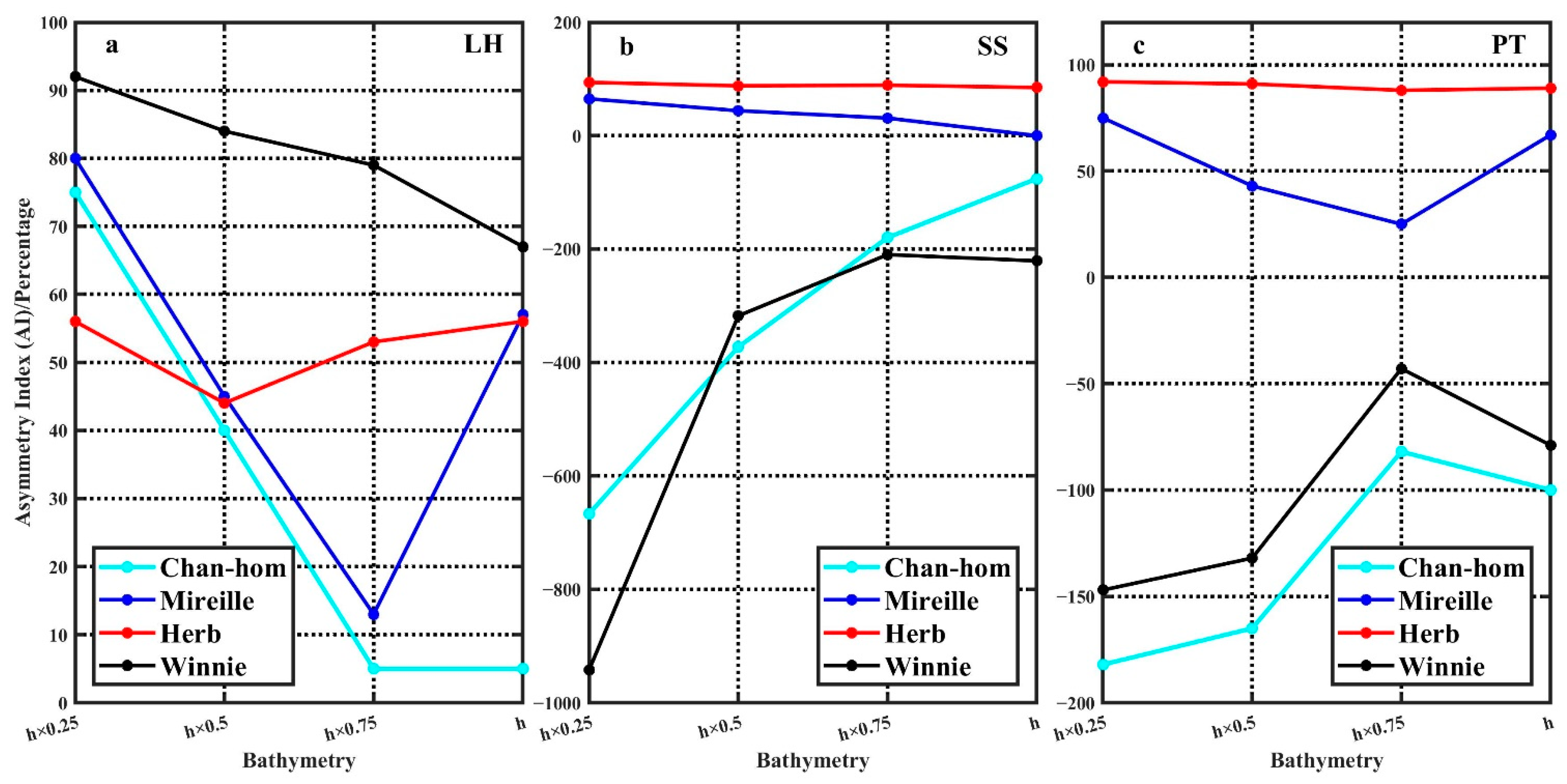
4.4. Effect of Topography

To explore the effect of topography on storm surges, another three sensitivity experiments were conducted in this section. Table 4 lists the details of each sensitivity experiment and Figure 19 draws the water depth contours of bathymetry configuration. In this section, water depth in sensitivity experiments is smaller than the original bathymetry to focus on the effect of decreasing bathymetry.

In Figure 20, the contour plots of Cases (5.1,5.4–5.6) show the effect of the topography of peak surges that happen at every mesh node over the entire simulation time of path Chan-hom. As the response of surge elevation to wind stress is inversely proportional to the water depth [25], a shallower water depth response to a higher surge elevation. It can be seen in Figure 20a (Case 5.1), the peak surge elevations are distributed along with the coastal areas, especially in the Hangzhou Bay, Yangtze River Estuary, and the coastal areas of Jiangsu Province and Zhejiang Province. The variations of peak surge elevations in different sensitivity experiments at every mesh node are shown in Figure 20b–d. Overall, large variations can be found in Hangzhou Bay and Yangtze River Estuary. The variations of surge elevations in Cases 5.4–5.6 have a similar pattern with Case 5.1; besides, the variation of surge elevation in Case 5.4 is the largest, and the variation of surge elevation in Case 5.6 is the smallest. The results indicate that the peak surge elevations increase with a decreasing slope, and surge elevations along the coastal area are easier to be affected.

Specifically, the time series of surge elevations at three stations that represent north (LH), middle (SS), and south (PT) of the SCC are calculated and shown in Figure 21. Overall, the peak surge elevations in sensitivity experiments are higher than the default values at these stations. Besides, the occurrence time of surge reaching the peak is longer than the time in default bathymetry, and a shallower bathymetry leads to a longer occurrence time of surge reaching the peak. Take path Chan-hom as an example. The Surge_max is 0.86 m at LH station in Case 5.1, and the values of Surge_max (or the variation of surge elevation compared with Case 5.1) are 1.90 (+1.04), 1.33 (+0.47), and 0.99 m (+0.13) in Cases 5.4–5.6. At PT station, the Surge_max is 0.13 m in Case 5.1, and the values of Surge_max (or the variation of surge elevation compared with Case 5.1) are 0.22 (+0.09), 0.17 (+0.04), and 0.17 m (+0.04) in Cases 5.4–5.6. Besides, the occurrence time of surge reaches the peak is 29 h at PT station in Case 5.1 (

Table 9. The model results of surge, fall, time and the value of AI in sensitivity experiments with different topography at three stations (LH, SS, and PT). Surge (m): Surge_max; fall (m): Fall_max; time: occurrence time of surge reaches the peak (from a cold start); AI: asymmetry index.

Case Name	LH				SS				PT
	Surge (m)	Fall (m)	Time (h)	AI (%)	Surge (m)	Fall (m)	Time (h)	AI (%)	Surge (m)	Fall (m)	Time (h)	AI (%)
5.1	0.86	−0.82	39	5	0.17	−0.30	15	−76	0.13	−0.26	29	−100
5.4	1.90	−0.47	39	75	0.15	−1.15	119	−667	0.22	−0.62	37	−182
5.5	1.33	−0.80	39	40	0.15	−0.71	102	−373	0.17	−0.45	33	−165
5.6	0.99	−0.94	39	5	0.15	−0.42	33	−180	0.17	−0.31	33	−82
6.1	0.21	−0.09	8	57	0.11	−0.11	21	0	0.12	−0.04	13	67
6.4	0.30	−0.06	72	80	0.23	−0.08	42	65	0.16	−0.04	79	75
6.5	0.22	−0.12	46	45	0.16	−0.09	45	44	0.14	−0.08	40	43
6.6	0.16	−0.14	49	13	0.13	−0.09	35	31	0.12	−0.09	25	25
7.1	0.16	−0.07	8	56	0.72	−0.11	35	85	0.88	−0.10	37	89
7.4	0.16	−0.07	37	56	2.28	−0.14	38	94	1.99	−0.15	38	92
7.5	0.18	−0.10	55	44	1.35	−0.16	37	88	1.44	−0.13	38	91
7.6	0.15	−0.07	52	53	0.89	−0.10	36	89	1.10	−0.13	37	88
8.1	0.48	−0.16	45	67	0.14	−0.45	35	−221	0.14	−0.25	37	−79
8.4	1.77	−0.15	45	92	0.19	−1.98	60	−942	0.30	−0.74	42	−147
8.5	1.0	−0.16	43	84	0.22	−0.92	36	−318	0.25	−0.58	39	−132
8.6	0.68	−0.14	43	79	0.20	−0.62	36	−210	0.21	−0.30	36	−43

), and the occurrence time of surges reach peak (or the variation of occurrence time of surge reaches peak compared with Case 5.1) are 37 (+8), 33 (+4) and 33 h (+4) in Cases 5.4–5.6. The cases with the other three paths (Mireille, Herb, and Winnie) have a similar pattern with the results of path Chan-hom. In addition, a shallower water depth could lead to a stronger asymmetry between Surge_max and Fall_max, which can be inferred from Figure 22.

5. Conclusions and Discussion

In this study, the effects of key parameters in the wind field and pressure field (forward speed, RMW, inflow angle, and central pressure), typhoon path, wind intensity, and topography on the modeling of storm surges and surge asymmetry along the SCC were investigated through numerical simulations. The combination of the Fujita pressure field and Takahashi pressure field model was employed to reconstruct the wind field and wind pressure of the typhoon. The model results agreed well with the observations during four typhoon processes (Chan-hom, Mireille, Herb, and Winnie), indicating that the parameters used in the model are appropriate and the model is reasonable to simulate the storm surges.

Asymmetry between the maximum sea level of surge and the maximum sea level of fall is studied in this paper. The idealized study in the paper provides a basic framework for the understanding of storm surges and surge asymmetry along the SCC. Overall, a larger forward speed could lead to a smaller peak surge elevation and a longer occurrence time of surge reaching the peak, as well as a longer duration time of high water in surge elevation. A larger RMW produces a higher sea level of surge and sea level of fall, and a larger RMW could lead to a lower value of surge asymmetry. Besides, there is no apparent difference in peak surge elevation when modifying the inflow angle in the wind field. However, the maximum sea level of fall decreases when increasing the inflow angle, which indicates that a larger inflow angle leads to stronger surge asymmetry. The model results show that the surge asymmetry increases with an increase of central pressure at LH, SC, SS, and PT stations. However, the relationship between forward speed and surge asymmetry is heterogeneous and depends on the value of forward speed. For the above four parameters in wind and pressure field, decreasing the forward speed and central pressure could lead to a longer duration time of high water in surge elevation while changing the RMW and the inflow angle has a minor impact on the duration time of high water in surge elevation.

Besides, the model results show that the storm surge is mainly induced by wind forcing. Based on the contribution to peak surge elevation at DJS, DH, and LH stations (Zhoushan Archipelago area), the paths can be sorted in descending order: Chan-hom, Winnie, Herb, and Mireille. The effect of the air pressure forcing is only evident for the path of Mireille. The nonlinear interaction between the wind forcing and the air pressure tends to weaken the peak surge elevation. Overall, the most dangerous path type is Chan-hom for the northern stations along the SCC, and the path of Winnie flows next.

The model results also indicate that there is a larger impact on peak surge elevation than the occurrence time of surge reaching the peak when changes the wind intensity. Besides, increasing (or decreasing) the wind intensity could increase (or decrease) the magnitude of wind velocity and the size of the wind field. The variation of surge elevation is a combined effect of wind intensity and size of the wind field. The relationship between surge asymmetry and wind intensity during four path simulations varies in path type. In general, for path Chan-hom, the values of surge asymmetry decrease with the increase of wind intensity; for path Mireille and Herb, a stronger wind field could lead to a strengthen of surge asymmetry; for path Winnie, the relationship between surge asymmetry and wind intensity is heterogeneous and varies with the stations.

Furthermore, decreasing bathymetry has a significant role in peak surge and the occurrence time of surge reaching the peak. The peak surge elevation increases with a decreasing slope, and peak values along the coastal area are easier to be affected. In general, a shallower water depth could lead to a stronger surge asymmetry.

Based on the model results in this paper, some implications of the proposed framework in decision process are summarized and shown as follows: for typhoons with the same wind intensity, a slower forward speed leads to a higher peak surge elevation and results in a greater threat to the coastal areas (Figure 5). As a result, for a slower forward speed typhoon, it needs to be taken seriously. Besides, the typhoon with large RMW and low central pressure is also a great threat to coastal communities. In addition, affected by global climate change, the frequency and intensity of storm surges have been increasing in recent decades. Furthermore, with land reclamation and more suspended sediment accumulated at the coastal area, such as the Hangzhou Bay and Yangtze River Estuary, the water depth becomes shallower in some coastal areas. For typhoon Chan-hom and Winnie (Figure 17 and Figure 21), increasing the wind intensity and decreasing the water depth could lead to a significant increasing of positive surge elevation at LH station (represents northern stations along SCC), while leading to a lower negative surge elevation at SS and PT station (represents middle and southern stations along SCC). As a result, for these two types of typhoons, more work should concentrate on the positive surge elevations at northern stations along SCC and the negative surge elevations at middle and southern stations along SCC. For typhoon Herb (Figure 17 and Figure 21), an intensified wind field and a shallower water depth could lead to a higher surge elevation at SS and PT stations, which indicates that more attention should be paid on the negative surge elevations at middle and southern stations along SCC in this typhoon type. Although this study was site-specific, it may be applicable for similar environments worldwide.

References

1. Kim, S.Y.; Yasuda, T.; Mase, H. Numerical analysis of effects of tidal variations on storm surges and waves. Appl. Ocean Res. 2008, 30, 311–322. [Google Scholar] [CrossRef]
2. Wolf, J. Coastal flooding: Impacts of coupled wave–surge–tide models. Nat. Hazards 2009, 49, 241–260. [Google Scholar] [CrossRef] [Green Version]
3. Li, C.; Weeks, E.; Blanchard, B.W. Storm surge induced flux through multiple tidal passes of Lake Pontchartrain estuary during Hurricanes Gustav and Ike. Estuar. Coast. Shelf Sci. 2010, 87, 517–525. [Google Scholar] [CrossRef]
4. Rego, J.L.; Li, C. Nonlinear terms in storm surge predictions: Effect of tide and shelf geometry with case study from Hurricane Rita. J. Geophys. Res. Oceans 2010, 115, C06020. [Google Scholar] [CrossRef] [Green Version]
5. Xu, J.; Zhang, Y.; Cao, A.; Liu, Q.; Lv, X. Effects of tide-surge interactions on storm surges along the coast of the Bohai Sea, Yellow Sea, and East China Sea. Sci. China Earth Sci. 2016, 59, 1308–1316. [Google Scholar] [CrossRef]
6. Heaps, N.S. Storm surges, 1967–1982. Geophys. J. Int. 1983, 74, 331–376. [Google Scholar] [CrossRef] [Green Version]
7. Zhang, W.Z.; Shi, F.; Hong, H.S.; Shang, S.P.; Kirby, J.T. Tide-surge interaction intensified by the Taiwan Strait. J. Geophys. Res. Oceans 2010, 115, C06012. [Google Scholar] [CrossRef] [Green Version]
8. Zhang, H.; Cheng, W.; Qiu, X.; Feng, X.; Gong, W. Tide-surge interaction along the east coast of the Leizhou Peninsula, South China Sea. Cont. Shelf. Res. 2017, 142, 32–49. [Google Scholar] [CrossRef]
9. Pranzini, E.; Wetzel, L.; Williams, A.T. Aspects of coastal erosion and protection in Europe. J. Coast. Conserv. 2015, 19, 445–459. [Google Scholar] [CrossRef]
10. Pope, J. Responding to coastal erosion and flooding damages. J. Coast. Res. 1997, 13, 704–710. [Google Scholar]
11. Arnell, N.W.; Gosling, S.N. The impacts of climate change on river flood risk at the global scale. Clim. Chang. 2016, 134, 387–401. [Google Scholar] [CrossRef] [Green Version]
12. Woth, K.; Weisse, R.; Von Storch, H. Climate change and North Sea storm surge extremes: An ensemble study of storm surge extremes expected in a changed climate projected by four different regional climate models. Ocean Dyn. 2006, 56, 3–15. [Google Scholar] [CrossRef]
13. Mel, R.; Sterl, A.; Lionello, P. High resolution climate projection of storm surge at the Venetian coast. Nat. Hazards Earth Syst. 2013, 13, 1135–1142. [Google Scholar] [CrossRef] [Green Version]
14. Rahmstorf, S. Rising hazard of storm-surge flooding. Proc. Natl. Acad. Sci. USA 2017, 114, 11806–11808. [Google Scholar] [CrossRef] [PubMed] [Green Version]
15. Mel, R.; Lionello, P. Verification of an ensemble prediction system for storm surge forecast in the Adriatic Sea. Ocean Dyn. 2014, 64, 1803–1814. [Google Scholar] [CrossRef]
16. Flowerdew, J.; Horsburgh, K.; Wilson, C.; Mylne, K. Development and evaluation of an ensemble forecasting system for coastal storm surges. Q. J. R. Meteor. Soc. 2010, 136, 1444–1456. [Google Scholar] [CrossRef] [Green Version]
17. Buizza, R.; Milleer, M.; Palmer, T.N. Stochastic representation of model uncertainties in the ECMWF ensemble prediction system. Q. J. R. Meteor. Soc. 1999, 125, 2887–2908. [Google Scholar] [CrossRef]
18. Chen, C.; Huang, H.; Beardsley, R.C.; Liu, H.; Xu, Q.; Cowles, G. A finite volume numerical approach for coastal ocean circulation studies: Comparisons with finite difference models. J. Geophys. Res. Oceans 2007, 112, 83–87. [Google Scholar] [CrossRef]
19. Rego, J.L.; Li, C. On the importance of the forward speed of hurricanes in storm surge forecasting: A numerical study. Geophys. Res. Lett. 2009, 36. [Google Scholar] [CrossRef] [Green Version]
20. Feng, X.; Yin, B.; Yang, D. Effect of hurricane paths on storm surge response at Tianjin, China. Estuar. Coast. Shelf Sci. 2012, 106, 58–68. [Google Scholar] [CrossRef]
21. Averkiev, A.S.; Klevannyy, K.A. A case study of the impact of cyclonic trajectories on sea-level extremes in the Gulf of Finland. Cont. Shelf Res. 2010, 30, 707–714. [Google Scholar] [CrossRef]
22. Musinguzi, A.; Akbar, M.K. Effect of varying wind intensity, forward speed, and surface pressure on storm surges of hurricane Rita. J. Mar. Sci. Eng. 2021, 9, 128. [Google Scholar] [CrossRef]
23. Zhang, X.; Chu, D.; Zhang, J. Effects of nonlinear terms and topography in a storm surge model along the southeastern coast of China: A case study of Typhoon Chan-hom. Nat. Hazards 2021, 1–24. [Google Scholar] [CrossRef]
24. Peng, M.; Xie, L.; Pietrafesa, L.J. Tropical cyclone induced asymmetry of sea level surge and fall and its presentation in a storm surge model with parametric wind fields. Ocean Model. 2006, 14, 81–101. [Google Scholar] [CrossRef]
25. Wong, B.; Toumi, R. Model study of the asymmetry in tropical cyclone-induced positive and negative surges. Atmos. Sci. Lett. 2016, 17, 334–338. [Google Scholar] [CrossRef] [Green Version]
26. Zhu, Y.; Ding, J.; Lu, M.; Wang, J.; Wang, Q. Analysis of the tropical cyclones landing in Zhejiang province during 1949–2009. Mar. Forecast. 2012, 29, 8–13. (In Chinese) [Google Scholar] [CrossRef]
27. Li, X.; Han, G.; Yang, J.; Chen, D.; Zheng, G.; Chen, N. Using satellite altimetry to calibrate the simulation of typhoon Seth storm surge off Southeast China. Remote Sens. 2018, 10, 657. [Google Scholar] [CrossRef] [Green Version]
28. Chu, D.; Zhang, J.; Wu, Y.; Jiao, X.; Qian, S. Sensitivities of modeling storm surge to bottom friction, wind drag coefficient, and meteorological product in the East China Sea. Estuar. Coast. Shelf Sci. 2019, 231, 106460. [Google Scholar] [CrossRef]
29. Chen, C.; Liu, H.; Beardsley, R.C. An unstructured grid, finite-volume, three dimensional, primitive equations ocean model: Application to coastal ocean and estuaries. J. Atmos. Ocean. Technol. 2003, 20, 159–186. [Google Scholar] [CrossRef]
30. Mellor, G.L.; Yamada, T. Development of a turbulence closure model for geophysical fluid problems. Rev. Geophys. 1982, 20, 851–875. [Google Scholar] [CrossRef] [Green Version]
31. Smagorinsky, J. General circulation experiments with the primitive equations: I. the basic experiment. Mon. Weather Rev. 1963, 91, 99–164. [Google Scholar] [CrossRef]
32. Large, W.G.; Pond, S. Open ocean momentum flux measurements in moderate to strong winds. J. Phys. Oceanogr. 1981, 11, 324–336. [Google Scholar] [CrossRef] [Green Version]
33. Holland, G.J. An analytic model of the wind and pressure profiles in hurricanes. Mon. Weather Rev. 1980, 108, 1212–1218. [Google Scholar] [CrossRef]
34. Jelesnianski, C.P.; Chen, J.; Shaffer, W.A. SLOSH: Sea, Lake, and Overland Surges from Hurricanes; US Department of Commerce, National Oceanic and Atmospheric Administration, National Weather Service: Silver Spring, MD, USA, 1992.
35. Chen, W.; Liu, W.; Hsu, M. Predicting typhoon-induced storm surge tide with a two-dimensional hydrodynamic model and artificial neural network model. Nat. Hazards Earth Syst. Sci. 2012, 12, 3799–3809. [Google Scholar] [CrossRef]
36. Zhang, W.; Hong, H.; Shang, S.; Chen, D.; Chai, F. A two-way nested coupled tide-surge model for the Taiwan Strait. Cont. Shelf Res. 2007, 27, 1548–1567. [Google Scholar] [CrossRef]
37. Ou, S.; Liau, J.; Hsu, T.; Tzang, S. Simulating typhoon waves by SWAN wave model in coastal waters of Taiwan. Ocean Eng. 2002, 29, 947–971. [Google Scholar] [CrossRef]
38. Ji, C.; Zhang, Q.; Wu, Y. An empirical formula for maximum wave setup based on a coupled wave-current model. Ocean Eng. 2018, 147, 215–226. [Google Scholar] [CrossRef]
39. Peng, M.; Xie, L.; Pietrafesa, L.J. A numerical study on hurricane-induced storm surge and inundation in Charleston Harbor, South Carolina. J. Geophys. Res. Oceans 2006, 111, C08017. [Google Scholar] [CrossRef] [Green Version]
40. Qiao, W.; Song, J.; He, H.; Li, F. Application of different wind field models and wave boundary layer model to typhoon waves numerical simulation in WAVEWATCH III model. Tellus A 2019, 71, 1657552. [Google Scholar] [CrossRef] [Green Version]
41. Wang, X.; Yi, Q.; Zhang, B. Research and applications of forecasting model of typhoon surges in China Seas. Adv. Water Sci. 1991, 2, 1–10. (In Chinese) [Google Scholar]
42. Yu, C.; Yang, Y.; Yin, X.; Sun, M.; Shi, Y. Impact of Enhanced wave-induced mixing on the ocean upper mixed layer during typhoon Nepartak in a regional model of the Northwest Pacific Ocean. Remote Sens. 2020, 12, 2808. [Google Scholar] [CrossRef]
43. Fujita, T. Pressure distribution within typhoon. Geophys. Mag. 1952, 23, 437–451. [Google Scholar]
44. Takahashi, K. Distribution of pressure and wind in a typhoon. J. Meteor. Soc. Jpn. 1939, 17, 417–421. [Google Scholar]
45. Willoughby, H.E. Gradient balance in tropical cyclones. J. Atmos. Sci. 1990, 47, 265–274. [Google Scholar] [CrossRef] [Green Version]
46. Ueno, T. Numerical computations of the storm surges in Tosa Bay. J. Oceanogr. Soc. Jpn. 1981, 37, 61–73. [Google Scholar] [CrossRef]
47. Graham, H.E.; Nunn, D.E. Meteorological Conditions Pertinent to Standard Project Hurricane; Report No. 3; Atlantic and Gulf Coasts of United States, National Hurricane Research Project; US Weather Service: Washington, DC, USA, 1959.
48. Allen, J.I.; Somerfield, P.J.; Gilbert, F.J. Quantifying uncertainty in high-resolution coupled hydrodynamic-ecosystem models. J. Mar. Syst. 2007, 64, 3–14. [Google Scholar] [CrossRef]
49. Murty, T.S.; Neralla, V.R. On the recurvature of tropical cyclones and the storm surge problem in Bangladesh. Nat. Hazards 1992, 6, 275–279. [Google Scholar] [CrossRef]
50. Bernier, N.B.; Thompson, K.R. Predicting the frequency of storm surges and extreme sea levels in the Northwest Atlantic. J. Geophys. Res. Oceans 2006, 111, C10009. [Google Scholar] [CrossRef] [Green Version]
51. Irish, J.L.; Resio, D.T. A hydrodynamics-based surge scale for hurricanes. Ocean Eng. 2010, 37, 69–81. [Google Scholar] [CrossRef]
Figure 1. The path of tropical cyclone for each type: (a) Chan-hom (type 1), (b) Mireille (type 2), (c) Herb (type 3), and (d) Winnie (type 4).
Jmse 09 00458 g001
Figure 2. (a) Bathymetry of the model and locations of tidal gauge stations (white inverted triangle), (b) computational meshes of the study domain.
Jmse 09 00458 g002
Figure 3. The horizontal schematic diagram of the wind field coordinate system. R: the radius of maximum wind; r: the radial distance from the typhoon center; θ: the inflow angle.
Jmse 09 00458 g003
Figure 4. Time series of observed and modeled sea surface elevation (Panel A) and surge elevation (Panel B) during four typhoons (Typhoon: Chan-hom, Mireille, Herb, Winnie).
Jmse 09 00458 g004
Figure 5. Time series of surge elevation in experiments with different forward speed at stations: (a) DJS, (b) DH, (c) LH, (d) SC, (e) SS, and (f) PT.
Jmse 09 00458 g005
Figure 6. The relationship among asymmetry index (AI) and forward speed (a,d), RMW (b,e), and inflow angle (c,f) at six stations.
Jmse 09 00458 g006
Figure 7. Time series of surge elevation in different RMW experiments at: (a) DJS, (b) DH, (c) LH, (d) SC, (e) SS, and (f) PT station.
Jmse 09 00458 g007
Figure 8. Time series of surge elevation in experiments with different inflow angle at: (a) DJS, (b) DH, (c) LH, (d) SC, (e) SS, and (f) PT station.
Jmse 09 00458 g008
Figure 9. Time series of surge elevation in experiments with different central pressure at: (a) DJS, (b) DH, (c) LH, (d) SC, (e) SS, and (f) PT.
Jmse 09 00458 g009
Figure 10. The relationship between asymmetry index and central pressure at: (a) DJS, DH, and LH stations; (b) SC, SS, and PT stations.
Jmse 09 00458 g010
Figure 11. Time series of surge elevations in experiments with different path at six stations: (a) DJS, (b) DH, (c) LH, (d) SC, (e) SS, and (f) PT.
Jmse 09 00458 g011
Figure 12. Model simulated wind field at time T1, T2, and T3 (at LH station) for the typhoon paths of Chan-hom (ac) and Winnie (df); model simulated wind field at time T1, T2 and T3 (at PT station) for the typhoon paths of Mireille (gi) and Herb (jl). The red line represents the typhoon path.
Jmse 09 00458 g012
Figure 13. Model simulated pressure distribution at time T1, T2, and T3 (at LH station) for typhoon paths of Chan-hom (ac) and Winnie (df); model simulated pressure distribution at time T1, T2, and T3 (at PT station) for typhoon paths of Mireille (gi) and Herb (jl). The red line represents the typhoon path.
Jmse 09 00458 g013
Figure 14. The path of Chan-hom (red solid line) and hypothetical paths (black solid lines).
Jmse 09 00458 g014
Figure 15. The time series of surge elevations with eight hypothetical paths at (a) DJS, (b) DH, (c) LH, (d) SC, (e) SS, and (f) PT station.
Jmse 09 00458 g015
Figure 16. The maximum wind velocity magnitude in (a) Case 5.1, (c) Case 5.2, and (e) Case 5.3; The maximum sea surface elevation in (b) Case 5.1, (d) Case 5.2, and (f) Case 5.3. The white line represents the path of Chan-hom.
Jmse 09 00458 g016
Figure 17. The time series of surge elevations in different wind intensity cases: (a1f1) Chan-hom, (a2f2) Mireille, (a3f3) Herb, and (a4f4) Winnie.
Jmse 09 00458 g017
Figure 18. The relationship between asymmetry index and wind intensity with different paths at: (a) DJS, (b) DH, (c) LH, (d) SC, (e) SS, and (f) PT station.
Jmse 09 00458 g018
Figure 19. Bathymetry in different cases: (a) default bathymetry, (b) original depth × 0.25, (c) original depth × 0.5, and (d) original depth × 0.75.
Jmse 09 00458 g019
Figure 20. (a) Contour plots of peak surges for the simulation of path Chan-hom in Case 5.1, and the red line is the path of Chan-hom; (bd) Contour plots of peak surge differences for the simulation of path Chan-hom between sensitivity experiments and Case 5.1, and the red line is the path of Chan-hom.
Jmse 09 00458 g020
Figure 21. The time series of surge elevations in cases with different topography settings: (a1c1) Chan-hom, (a2c2) Mireille, (a3c3) Herb, and (a4c4) Winnie.
Jmse 09 00458 g021
Figure 22. The relationship between asymmetry index and bathymetry during four paths simulations at: (a) LH, (b) SS, and (c) PT station.
Jmse 09 00458 g022