Decadal Assessment of Sperm Whale Site-Specific Abundance Trends in the Northern Gulf of Mexico Using Passive Acoustic Data

Abstract

Passive acoustic monitoring has been successfully used to study deep-diving marine mammal populations. To assess regional population trends of sperm whales in the northern Gulf of Mexico (GoM), including impacts of the Deepwater Horizon platform oil spill in 2010, the Littoral Acoustic Demonstration Center-Gulf Ecological Monitoring and Modeling (LADC-GEMM) consortium collected broadband acoustic data in the Mississippi Valley/Canyon area between 2007 and 2017 using bottom-anchored moorings. These data allow the inference of short-term and long-term variations in site-specific abundances of sperm whales derived from their acoustic activity. A comparison is made between the abundances of sperm whales at specific sites in different years before and after the oil spill by estimating the regional abundance density. The results show that sperm whales were present in the region throughout the entire monitoring period. A habitat preference shift was observed for sperm whales after the 2010 oil spill with higher activities at sites farther away from the spill site. A comparison of the 2007 and 2015 results shows that the overall regional abundance of sperm whales did not recover to pre-spill levels. The results indicate that long-term spatially distributed acoustic monitoring is critical in characterizing sperm whale population changes and in understanding how environmental stressors impact regional abundances and the habitat use of sperm whales.

1. Introduction

Sperm whales and other deep-diving marine mammal species produce powerful sounds for echolocation, foraging, and communication [1,2,3,4,5,6]. In the last two decades, several reliable and well-established survey methods have been used to characterize marine mammal behavior and abundance trends such as visual observations, tagging, and passive acoustic monitoring techniques [7,8,9,10,11,12,13,14,15,16,17,18,19,20,21,22]. These techniques are becoming more common in studying the behavior of marine mammals. Although visual observations can identify the presence of marine mammals near the ocean surface and lead to the identification of individuals, they provide no insight into the presence of whales, foraging behavior, or feeding success during deep dives. Visual observations are also limited to daylight times and calm weather conditions. By using acoustic tag data, researchers can obtain information about dive profiles, foraging behavior, and acoustic activity. However, only a small subset of animals gets tagged and the efforts are expensive and time consuming. A few species (e.g., beaked whale species) are very difficult to approach and tag. Passive acoustic monitoring techniques provide a good alternative to simultaneously study many marine mammal species. Passive acoustic systems can record data continuously over long periods and large areas without human involvement. At present, passive acoustic observations have been successfully used to detect and analyze underwater acoustic signals produced by different marine mammals including Gulf of Mexico (GoM) sperm whales, beaked whales, and dolphins [5,6,7,9,10,23,24,25].

To assess local abundance trends of marine mammals in the northern Gulf of Mexico, the Littoral Acoustic Demonstration Center-Gulf Ecological Monitoring and Modeling (LADC-GEMM) consortium conducted a series of passive acoustic surveys in the area between 2007 and 2017. One of the research goals was to investigate the impact of the 2010 Deepwater Horizon (DWH) oil spill (20 April 2010–19 September 2010) on the residential population of sperm whales in the northern GoM. Prior to the 2010 oil spill, LADC-GEMM had already collected acoustic data near the oil spill site to study GoM marine mammals using acoustics-based methods [26,27,28,29]. Starting in 2010, the LADC-GEMM consortium redeployed passive acoustic monitoring systems at previous sites to assess the impact of the oil spill on the regional populations of marine mammals [5].

The objective of this paper is to study regional site-specific abundance trends of sperm whales in the past decade and to better understand how abundance variability depends on seasons, locations, and environmental conditions.

The remainder of this paper is organized as follows. Section 2 describes the experiment. Section 3 describes the details of the acoustic data processing to detect sperm whale clicks [30] and the density estimation methodology based on the approach developed by Marques et.al [21]. Section 4 presents the results and discussions. The conclusions are drawn and future research directions are outlined in Section 5.

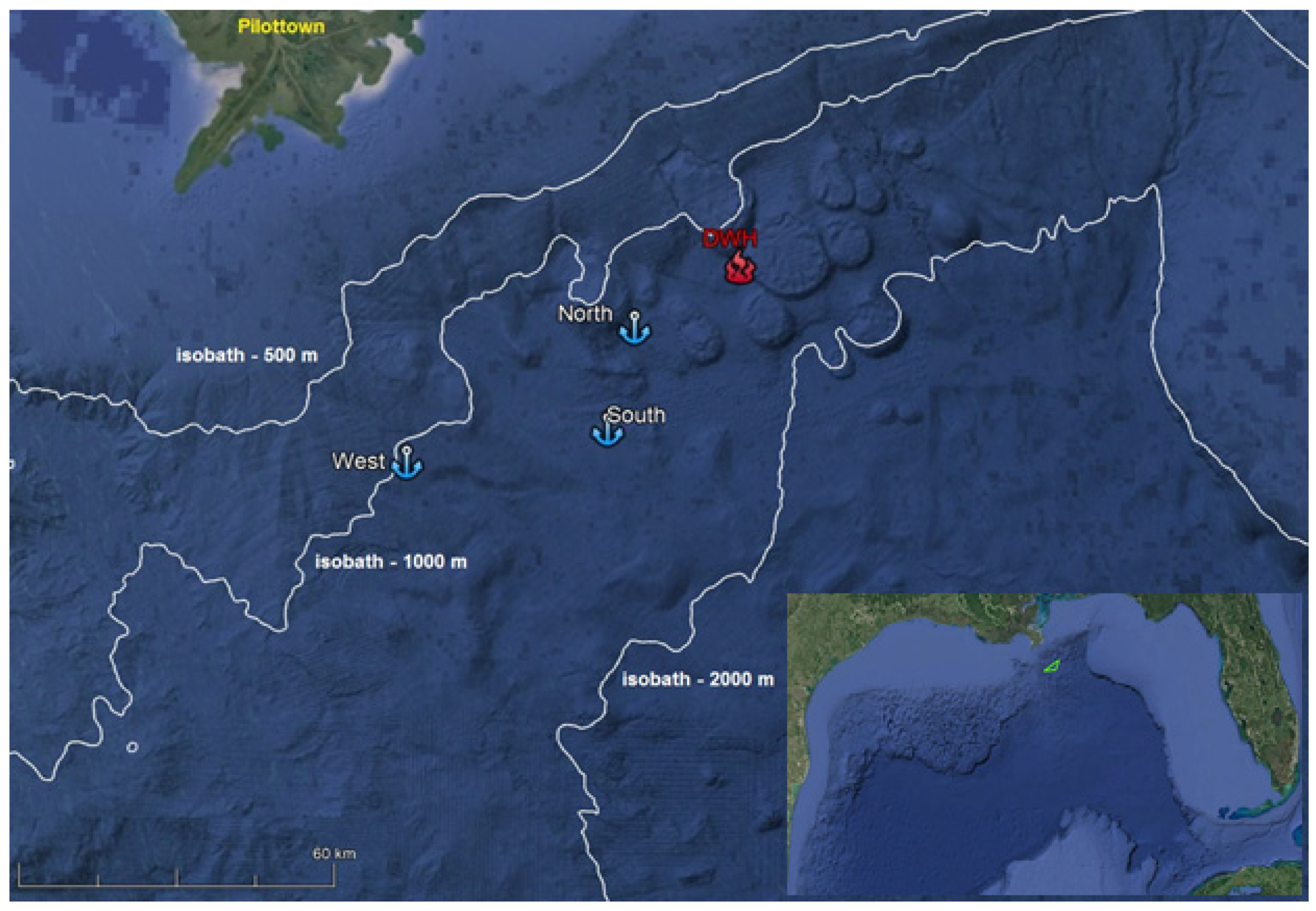
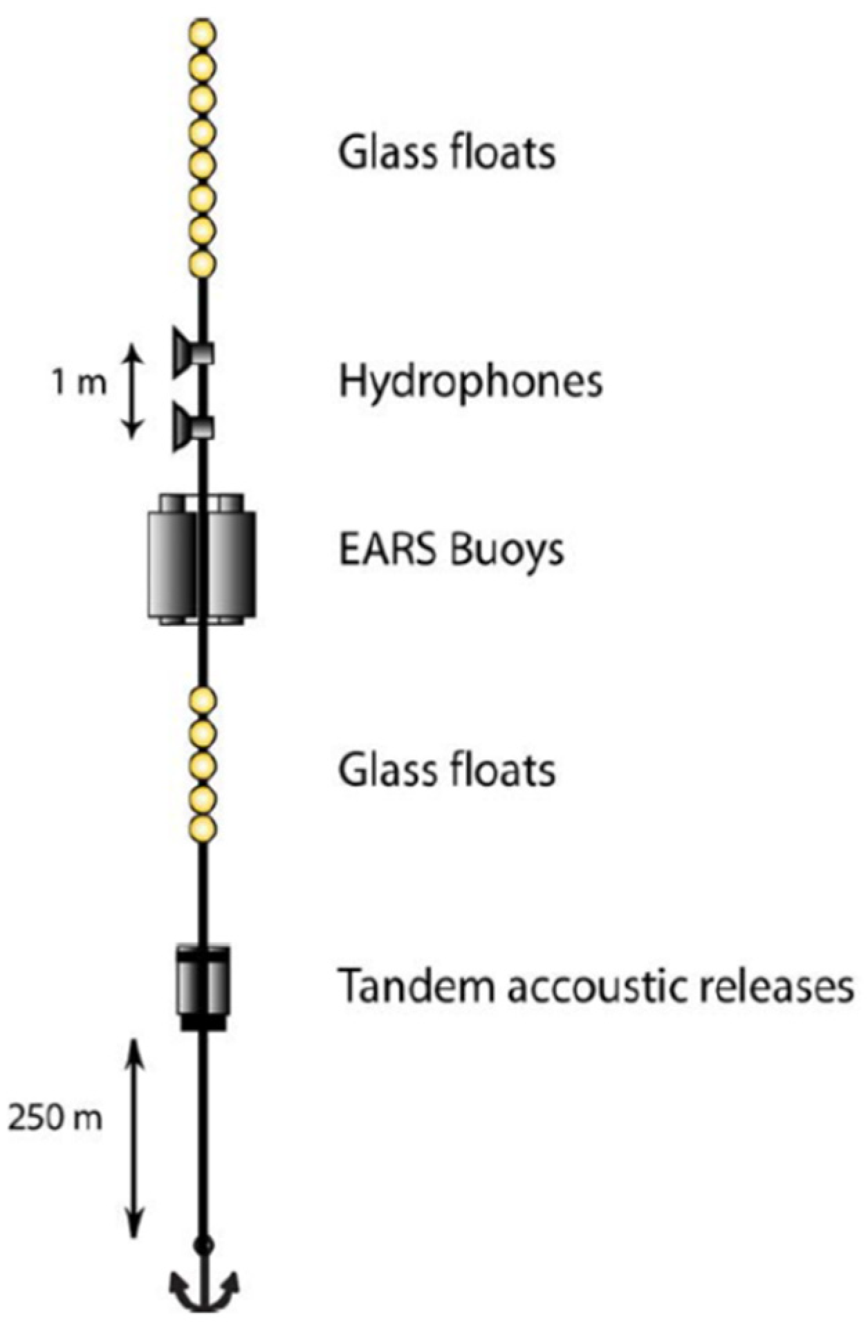
2. Experiment and Data Collection

The LADC-GEMM consortium collected several passive acoustic datasets in the northern GoM in the past decade as part of long-term monitoring efforts. Acoustic recordings were collected at three different sites, further referred to as the Northern (N), Southern (S), and Western (W) sites (shown in Figure 1). The sites were about 16, 40 and 80 km away from the oil spill site, respectively. At each site, one or more bottom-anchored deepwater moorings containing an Environmental Acoustic Recording System (EARS) buoy were deployed. The acoustic data were collected in 2007 (active recording period between 6 July and 16 July at the Northern and Southern sites), 2010 (active recording period between 10 September and 23 September at all three sites), 2015 (active recording period between 26 June and 22 October at all three sites), 2016 (active recording period between 10 September and 30 January 2017 at the Southern site) and 2017 (active recording period between 9 June and 9 October at all three sites), respectively.

Table 1. Geographic locations of EARS buoy moorings and the start/deployment and end/retrieval dates.

Year/Station	Latitude (N)	Longitude (W)	Water Depth (m)	Start	End
2007 North	28°38.99′	88°31.56′	1560	6 July	16 July
2007 South	28°25.23′	88°37.07′	1465	7 July	16 July
2010 North	28°39.00′	88°31.53′	1545	10 Sept	22 Sept
2010 South	28°24.61′	88°34.26′	1550	11 Sept	23 Sept
2010 West	28°23.06′	88°59.52′	1000	12 Sept	24 Sept
2015 North	28°39.07′	88°31.05′	1570	26 June	22 Oct
2015 South	28°25.28′	88°37.11′	1500	25 June	21 Oct
2015 West	28°24.04′	88°59.69′	1000	24 June	21 Oct
2016 South	28°27.71′	88°36.30′	1500	10 Sept	30 Jan
2017 North	28°38.09′	88°33.17′	1500	09 June	09 Oct
2017 South	28°27.63′	88°36.16′	1500	11 June	09 Oct
2017 West	28°23.84′	88°59.23′	1000	10 June	09 Oct

summarizes the details of each survey year and site deployment.

The EARS buoys were continuously recording acoustic data at a 192 kHz sampling rate. The data were stored on internal hard drives using a 16-bit analogue-to-digital converter. Using EARS and hydrophone calibration parameters, the recorded digitized data were later converted to pressures (in microPascals, µPa). For each deployment, the mooring included two paired single-channel EARS buoys; each buoy was connected to a hydrophone with an external cable providing a 1 m hydrophone separation for future localization studies (not discussed in this paper). Figure 2 shows a schematic of the EARS mooring used in the experiment. The moorings were deployed in different water depths at three sites, as shown in Table 1. The hydrophone depths were chosen to target the foraging depth of marine mammals (such as sperm and beaked whales) and to maximize the probability of recording their directional clicks.

3. Methods

Sperm whale clicks are typically emitted in series of tens to hundreds of clicks with a regular or regularly changing repetition rate [2]. These clicks include regular clicks for localization and long-range prey echolocation, buzzes for short-range prey echolocation, and codas for communication [2,3,14,31]. A typical sperm whale click train and associated spectrogram are shown in Figure 3. The interclick interval (ICI) varied between 0.5 and 2 s [4]. The main acoustic energy of clicks was in a frequency band between 3 and 20 kHz. The time series and spectrogram showed that a higher amplitude direct-path click was followed by lower amplitude clicks from surface- or bottom-reflected paths.

In general, a sperm whale click may contain three or more distinct pulses depending on the angle between the acoustic axis of a whale’s head and the propagation direction to a hydrophone due to internal reflections occurring in the head. A single click spectrum has multiple peaks and notches in the frequency band that can be used to determine the animal size and separate individuals in a group [32,33,34,35,36,37,38,39,40,41]. The time spacing between the pulses in a single click is referred to as the interpulse interval (IPI); three or more pulses may be found in a click. The IPI is related to the size of the sperm whale. The value of the IPI varies from 2 ms to 10 ms [40] depending on the size/age of the whales. The duration of a click may reach 20 to 30 ms [2]. Caruso et al. [40] used the IPI to estimate the size distribution of sperm whales detected by a deep hydrophone platform to obtain information on the population structure (size and age/sex) and also to understand changes in a sperm whale population over time. The duration of a click depends on the number of received pulses, which depends on the whale’s orientation relative to a receiver.

3.1. Population Density Estimation

A method of regional site-specific abundance density estimation from sperm whale clicks detected in the EARS continuous datastream was based on the methodology proposed by Marques et al. [17,21]:

$$\widehat{D}=\frac{n_c\left(1-\widehat{c}\right)}{K\pi w^2{\widehat{P}}_{d}T\widehat{r}}$$

(1)

where n_c is the number of detected cues over a time period, T (a cue is defined here as a foraging click), $\widehat{c}$ is the estimated proportion of false positive detections, w is the distance away from the hydrophones beyond which cues are assumed not to be detected (the maximum cue detection range), ${\widehat{P}}_d$ is the estimated average probability of detecting a cue out to distance w, $\widehat{r}$ is the estimated cue production rate by a single mammal and K is the number of hydrophones used for a common detection range (K = 1 for this study). Formula (1) yields a point estimate of the population density of the animals within the detection region of the hydrophone.

3.2. Click Detection

In order to detect the acoustic signals of sperm whales and other marine mammal clicks, we developed a multiband spectral energy detection algorithm that was described in detail by Li et al. [30] in the context of detecting and classifying beaked whale clicks. The algorithm tracked received acoustic energy in several representative frequency bands. Clicks from different marine mammal species were discriminated by comparing energy against baseline levels in the bands of interest: low band (3–20 kHz), medium band (25–55 kHz), and high band (60–90 kHz). For the potential detection of sperm whale species, energy was required to be above the background level by a user-specified threshold only in the frequency band of 3–20 kHz. This approach allowed the initial discrimination of sperm whale clicks from beaked whale clicks (when energy was above the threshold in the medium band) and dolphin clicks (when energy was above the thresholds in all three bands).

The details of sperm whale click detection and counting were as follows. First, for a given time series of acoustic data, a short-time Fourier transform was calculated using a 512 point (2.7 ms) Hamming window with no overlap. Choosing a short FFT window without overlap was based on the practical matter of computation time and to minimize file size: the FFT window without overlap compressed the data by a few orders of magnitude. Furthermore, click detection results matched those of a human expert analysis, therefore it was satisfactory for use.

The value of the sum of the squared spectral amplitudes within each of the three bands of interests for each time window was saved, creating what was referred to as the spectral sum time series. Marine mammal clicks often appear as periodic peaks in the spectral sum time series. The mean and standard deviations of spectral sums were calculated over 10 min time intervals in each band of interest and used to set dynamic detection thresholds. A 10 standard deviation value above the 10 min mean for each band in this study were used as detection thresholds. The thresholds could change every 10 min depending on the acoustic background variability and were unique for each band. Figure 4 shows the spectral sum time series for the 3–20 kHz band with potential sperm whale detections marked by red dots. A potential sperm whale click was defined as any point where the spectral sum exceeded a threshold of 10 standard deviations above the mean in the low frequency band but was below the calculated thresholds in the medium and high bands. The 10 standard deviation threshold allowed the detection of clicks (based on the empirical human inspection and experience) that were assumed to be direct acoustic paths while ignoring the smaller amplitude clicks that were multipath acoustic arrivals (surface- and bottom-reflected paths). When searching for sperm whale clicks, a click event must be present only in the low frequency band. A concurrent detection in the medium frequency or high frequency bands disqualified it as a sperm whale click and the click event was discarded.

To lower the impact of ship noise and other manmade signals that might exist in the low frequency band and cause a high false detection rate, we set restrictions for the frequency and bandwidth of each potential click marked at the spectral energy detection step. For each potential click in the spectral sum time series, the algorithm extracted the peak frequency and bandwidth and fed them into the discriminator algorithm:

(i) if the peak frequency was not within 3–20 kHz, a click was disqualified as a sperm whale click;

(ii) if the bandwidth (measured at a −10 dB level below the peak of the power spectral density level) was not between 2 and 18 kHz, a click was disqualified as a sperm whale click. The criteria were based on prior knowledge of sperm whale click properties published in peer-reviewed literature [42].

The total number of detected clicks over the specified time interval (T) was then passed to the statistical model Equation (1), which was used for density estimation.

3.3. False Positive Rate

The parameter describing the proportion of false positive detections, $\widehat{c}$, was estimated by a manual examination of a 10 min interval every two hours across the entire dataset duration for each buoy and each survey period. The average false positive rate for each survey year at each location was used for density estimation.

3.4. Probability of Detection

The probability of detection was estimated by using the Monte Carlo simulation methodology proposed by Küsel et al. [19]. The signal-to-noise ratio (SNR) of received sperm whale clicks could be expressed by the source level (SL, measured in dB re 1 µPa at 1 m), directivity loss (DL, in dB), transmission loss (TL, in dB), and the ambient noise level (NL, measured in dB re 1 µPa) as [43]:

$$SNR=SL-DL-TL-NL$$

(2)

The SL was the sperm whale’s on-axis source level. The average source level of 235 ± 0.5 dB re 1 µPa rms [2] was chosen as the sperm whale’s on-axis source level.

The directivity loss (DL) could be obtained by calculating the off-axis attenuation of the source level [19]. The off-axis attenuation of the source level as a function of the off-axis angle for a sperm whale could be estimated by using a piston model [19,44] as follows:

$$P\left(\theta ,f\right)=P_0\frac{2J_1\left(x\right)}{x}$$

(3)

$$x=\frac{2\pi a\sin \left(\theta \right)f}{c}$$

(4)

where P represented pressure, P₀ was a reference source level, J₁ was the Bessel function of the first kind, f was the frequency, a was the piston radius, θ was the off-axis angle, and c was the speed of sound in the water.

The piston model was used to calculate the broadband beam pattern, which could be estimated by integrating $P\left(\theta ,f\right)$ with respect to the frequency. The broadband beam pattern was given by [44]:

$$B\left(\theta \right)=\frac{{\int }_{-\infty }^{\infty }P\left(\theta ,f\right)W^2\left(f\right)df}{{\int }_{-\infty }^{\infty }{W}^2\left(f\right)df}$$

(5)

where $W\left(f\right)$ was the Gaussian weighting function, which was given by:

$$W\left(f\right)=\exp \left\{-\frac{1}{2}{\left(\frac{f-f_0}{b}\right)}^2\right\}$$

(6)

where $f_0$ and b were the center frequency and rms bandwidth, respectively.

Once the broadband beam pattern was obtained, the directivity index (DI) could be estimated by integrating the modeled broadband beam pattern as follows [44]:

$$DI=10log\left(\frac{B\left(0\right){\int }_0^{\pi }sin\theta d\theta }{{\int }_0^{\pi }B\left(\theta \right)sin\left(\theta \right)d\theta }\right)$$

(7)

Table 2. Parameters for estimating sperm whale click directivity loss.

Parameter	Value
Reference source level	235 1
(dB re 1 µPa)
Piston radius a (cm)	80 1
Sound speed c (m/s)	1500
Frequency range f (kHz)	3–20
Center frequency f0 (kHz)	13.4 1
RMS bandwidth b (kHz)	4.1 1

¹ Parameters suggested by Møhl et al. [2].

summarizes the parameters used in this study for the sperm whale directivity loss calculations.

The transmission loss (TL) was modeled by taking into account spherical spreading and absorption loss [43]:

$$TL=20\log \left(r\right)+{\alpha }_f\frac{r}{1000}$$

(8)

where r was the range between a hypothetical source and receiver in the Monte Carlo simulations and ${\alpha }_f$ was the absorption coefficient expressed in dB/km.

The absorption coefficient could be expressed as [45]:

$${\alpha }_f\approx 3.3\times {10}^{-3}+\frac{0.11f^2}{1+f^2}+\frac{44f^2}{4100+f^2}+3.0\times {10}^{-4}{f}^2$$

(9)

The value for ${\alpha }_f$ was 2.01 dB/km (corresponding to a frequency of 13.4 kHz) as used for the transmission loss calculation.

The ambient noise level (NL) was measured by taking data with minimal sperm whale clicks and anthropogenic noise present by manual inspection. The ambient noise levels were estimated by calculating the mean of the ambient noise power of the data between 3 and 20 kHz in the 24 h period on each hydrophone.

Once all parameters in the sonar equation were obtained, the estimated SNR could be used to model the probability of detection used in the Monte Carlo simulations [19]. The SNRs in this study were randomly simulated for 10,000 clicks using hypothetical animal placement and acoustic axis orientation plus 100 iterations to generate detection probability uncertainty. For each experimental year at each location (Northern, Southern, and Western sites), a 10 min data sample having ample sperm whale clicks was selected. Each click in the data sample was manually marked by an analyst to characterize the detector performance at different SNRs. The probability of detection versus the SNR could be obtained by analyzing the detectability as a function of the measured SNR. The simulated SNRs were then used to estimate the probability of detecting sperm whale clicks. The probability of detection as a function of the SNR could be obtained by assigning the probability of detection corresponding with the detector characterization [19]. Finally, the probability of detection as a function of range could be obtained by converting the probability of detection versus the SNR into the probability of detection versus the range. The average probability of detecting a click within w was then obtained by integrating the product of detection function and the distribution of the horizontal object function [17] over the interval (1, w). The distribution of the horizontal object function was given by $\mathrm{h}\left(\mathrm{y}\right)=2\mathrm{y}/{\mathrm{w}}^2$, where y referred to the horizontal distance. The probability of detection (${\widehat{P}}_d$) for each survey year at each location is presented in Section 4.

3.5. The Maximum Detection Range

The maximum detection range could be obtained from the probability of detection as a function of range. Figure 5 shows the estimated probability of detection curves of sperm whales as a function of range for the 2015 acoustic dataset at the Northern, Southern, and Western sites, respectively.

Figure 5 illustrates that the modeled maximum detection range was about 25 km, so the maximum detection range, w, in Equation (1) was set to 25 km to estimate the population density and to ensure that on-axis clicks were accounted for longer propagation ranges.

The probability of detection curves at the three sites exhibited differences due to local ambient noise levels and local propagation conditions [46]. These differences were taken into account when the probability of detection was calculated for each site each year.

3.6. Production Rate

The click production rate, $\widehat{r}$, gave the average number of clicks produced per unit time per animal. Click production rates varied with time and location of the acoustic survey [47]. Several published studies have proposed methods for estimating the production rates for different types of marine mammals such as sperm whales and beaked whales [7,17,19,24,47,48,49].

As a first step in the absence of tagged animals, click production rate could be estimated by taking the inverse of the mean ICI. However, according to the tagged data recorded over a typical dive of a sperm whale [31], sperm whale clicks are only produced during the vocally active phase of the dive. Thus, using the inverse of the mean ICI as an estimate of click production rate would result in an overestimated parameter. Therefore, click production rate could be adjusted by taking into account the duration of the active clicking part of the dive cycle:

$$\widehat{r}=\frac{t_v-t_b}{t_{dive}}\times \frac{1}{ICI}$$

(10)

where $t_{dive}$ represented the duration of the dive cycle, $t_v$ represented the vocal duration of the dive, t_b represented the time spent producing buzzes during a deep dive, and ICI was the mean interclick interval from the detector.

The dive duration of a typical sperm whale is about 45 min and the vocal duration is about 37.4 min with a standard deviation of 7.4 min as obtained from tagged sperm whales [31]. The buzz producing time, t_b can be obtained from the product of the average number of buzzes, N_b, and the average length of each buzz, L_b. In this study, N_b was estimated to be 17 per dive with a standard deviation of 8.6 as introduced by Watwood et al. [31], and L_b was 5 s as suggested by Fais et al. [50]. Thus, we obtained $t_b$ = 1.42 min. The mean ICI in this study was estimated by taking the average of the time intervals between two consecutive detected clicks subject to the condition that the separation between the two consecutive clicks was greater than 0.030 s and less than 2 s in order to be used to calculate intervals between successive clicks.

The production rate was estimated for each site for each survey year due to the variability of the ICI between different locations.

3.7. Time Period

The processed time duration used in estimating the density population was set to 45 min, which corresponded with a single dive cycle in the foraging phase [31].

3.8. Variance of Density Estimates

To investigate the variance of the density estimations, a non-parametric bootstrap method described in Ackleh et al. [5] was used. The interval estimation of $\widehat{D}$ to obtain the accuracy of estimates was different from the one followed by Marques et al. [17] where the authors used the first order delta (FOD) method to approximate the variance of $\widehat{D}$. The approach implemented in [17] would lead to:

$$var\left(\widehat{D}\right)\approx {\widehat{D}}^2\left[\frac{Var\left(n_c\right)}{{(E\left(n_c\right))}^2}+\frac{Var(\left(1-\widehat{c}\right)}{{(E\left(1-\widehat{c}\right))}^2}+\frac{Var\left(\widehat{r}\right)}{{\left(E\left(\widehat{r}\right)\right)}^2}+\frac{Var\left({\widehat{P}}_d\right)}{{\left(E\left({\widehat{P}}_d\right)\right)}^2}\right]$$

(11)

The data collection method in [17] was different from this study because several animals were simultaneously tagged in their study. Tagged data allowed direct estimations of variances of individual parameters on the right-hand side of Equation (11). Due to the lack of tagged data, a bootstrap technique was proposed for estimating the variance of $\widehat{D}$ for this study. Equation (1) gave only a point estimate of the site density at a specific location of area. $\widehat{D}$ in (1) was an instantaneous density estimate over a period of time, T. Hence, interval estimates of the site density were obtained by employing the bootstrap approach described in detail in [5]. A total of 5000 iterations at each site and each survey period were implemented to generate the uncertainty and average population density with a 95% confidence interval.

4. Results and Discussion

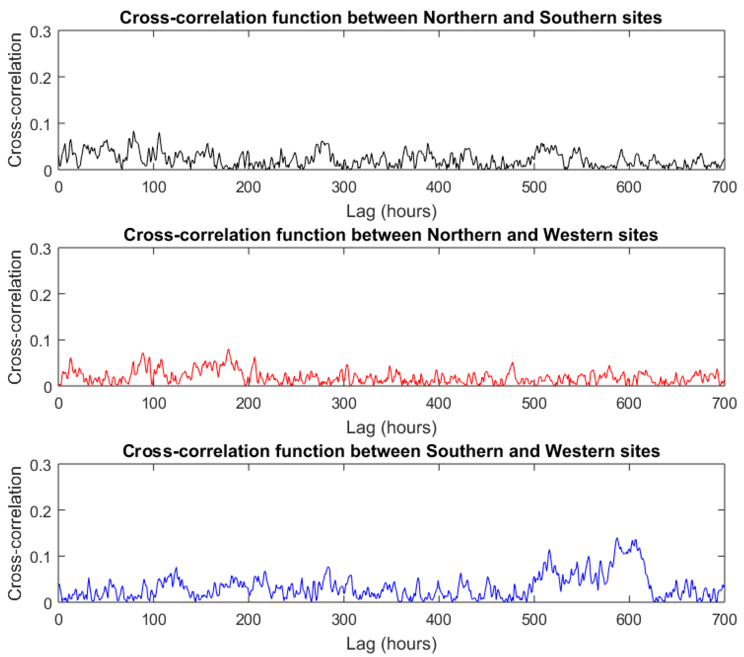
4.1. Sperm Whale Detections

Table 3. Average number of detected clicks in 45 min ($n_c$ ), false positive rate ($\widehat{c}$ ) and probability of detection (${\widehat{P}}_d$ ) at three sites for each survey year.

Year	Northern Site			Southern Site			Western Site
	${\mathit{n}}_{\mathit{c}}$	$\widehat{\mathit{c}}$	${\widehat{\mathit{P}}}_{\mathit{d}}$	${\mathit{n}}_{\mathit{c}}$	$\widehat{\mathit{c}}$	${\widehat{\mathit{P}}}_{\mathit{d}}$	${\mathit{n}}_{\mathit{c}}$	$\widehat{\mathit{c}}$	${\widehat{\mathit{P}}}_{\mathit{d}}$
2007	421.72	0.090	0.106	205.32	0.217	0.108	n/a	n/a	n/a
2010	85.49	0.156	0.081	316.60	0.071	0.056	232.43	0.071	0.055
2015	159.81	0.115	0.085	121.24	0.117	0.072	189.91	0.137	0.054
2016	n/a	n/a	n/a	264.70	0.070	0.067	n/a	n/a	n/a
2017	288.54	0.120	0.072	231.90	0.080	0.056	213.94	0.069	0.062

shows the average number of detected sperm whale clicks over a 45 min window (with an 80% overlap between two consecutive windows) using the detection method described above at the Northern, Southern, and Western sites for each survey year. The average was taken over the entire monitoring period. The estimated proportion of false positives and the probability of click detection are also presented in Table 3.

To investigate the daily and site-specific acoustic activity variability related to a particular site usage, a 24 h average number of sperm whale clicks in every minute, referred to as the average daily click rate on each site, was calculated for each survey year. The average daily click rates of sperm whales at three sites (Northern, Southern, and Western sites) in 2015 over a 110-day observational period from July to October are shown in Figure 6.

Figure 6 shows that all sites were used during the entire monitoring period. The daily site utilization fluctuated throughout the entire monitoring period and none of the sites showed a strong seasonal preference during summer and fall. Similar dynamics were observed for 2017.

To further investigate regional movements of sperm whales and understand the family clan structure, Figure 7 shows the cross-correlation function for 1-hour detected click numbers between two site pairs.

One can conclude from Figure 7 that the cross-correlation coefficient (zero lag value) for detections was close to zero for each two-site pair. That was indicative that the sites were not used simultaneously by different groups. Thus, each site could be used to estimate regional abundance independently. The cross-correlation functions between the two sites showed local maxima that suggested sperm whale group movements across different sites.

Table 4. Estimated mean interclick interval (ICI), standard deviation (std) and click production rates ($\widehat{r}$ ) at three sites for each survey year.

Year	Northern Site			Southern Site			Western Site
	ICI	Std	$\widehat{\mathit{r}}$	ICI	Std	$\widehat{\mathit{r}}$	ICI	Std	$\widehat{\mathit{r}}$
2007	0.7017	0.4160	1.1396	0.7085	0.4186	1.1286	n/a	n/a	n/a
2010	0.7373	0.4397	1.0845	0.7169	0.4236	1.1154	0.7439	0.4074	1.0749
2015	0.7697	0.4288	1.0389	0.7924	0.4152	1.0091	0.7488	0.4214	1.0679
2016	n/a	n/a	n/a	0.7492	0.4138	1.0673	n/a	n/a	n/a
2017	0.7516	0.4276	1.0639	0.7481	0.4236	1.0689	0.7349	0.4222	1.0881

shows the estimated interclick interval (ICI) and click production rates ($\widehat{r}$) at the three sites for each survey year. The ICIs and click production rates ($\widehat{r}$) varied slightly with time and location. The site-specific ICI and $\widehat{r}$ were used for density estimates.

4.2. Regional Population Density Estimates

Figure 8a shows the estimated average site-specific density of sperm whales at the Northern, Southern, and Western sites across all survey years.

The sperm whale site-specific density estimates were related to the site used by sperm whale groups present in the region. In 2017 (seven years after the spill) the site-specific density estimates were similar across the three sites, which might be indicative of prey field recovery at the Northern site heavily exposed to leaked oil. In 2017, the average density across the three sites was estimated as 0.616 per 1000 km² and could be used as a regional population density measure. The limited tag data available for the GoM sperm whales have shown that a whale can swim between sites in less than one day and 100 km ranging is typical for the GoM groups [51], so a uniform site usage was expected unless there were uneven prey resources. Comparing the density estimates prior to (2007) and post (2015, 2017) the oil spill, the population density of sperm whales showed a significant decline near the oil spill site in 2010 immediately after the spill. The average density estimates in the Northern site went from 0.599/1000 km² in 2007 to 0.128/1000 km² in 2010. Meanwhile, the population density of sperm whales increased in the Southern site from 2007 to 2010. The average density estimates at the Southern site increased by 257% from 2007 to 2010. The results indicated that sperm whales probably left the Northern site area, which was in close proximity to the spill, and relocated to the other sites. That may explain the increase at the Southern site. A high concentration of pollutants and prey unavailability were quite likely the cause. By comparing the density estimates in 2010 and 2015, average density of sperm whales at the Northern site increased by 136% from 2010 (0.128/1000 km²) to 2015 (0.302/1000 km²). The results indicated that the density of sperm whales at the site closest to the spill showed recovery from 2010 to 2015, so animals increased the site occupancy, probably due to prey field recovery. A comparison of the densities in 2015 with the densities in 2017 across the same monitoring season showed that the average density in 2017 increased by 111.9%, 144.0%, and 3.47% at the Northern, Southern, and Western sites, respectively. The average site-specific density of sperm whales for each survey year and their associated coefficient of variations (CV) are quantitatively summarized in

Table 5. Average population density estimates ($\widehat{D}$ ) and CVs for sperm whales at the Northern, Southern and Western sites for each survey year.

Year	Northern Site		Southern Site		Western Site
	$\widehat{\mathit{D}}$ (/1000 km2)	CV	$\widehat{\mathit{D}}$ (/1000 km2)	CV	$\widehat{\mathit{D}}$ (/1000 km2)	CV
2007	0.599	0.021	0.249	0.034	n/a	n/a
2010	0.128	0.068	0.888	0.027	0.698	0.028
2015	0.302	0.010	0.275	0.013	0.518	0.009
2016	n/a	n/a	0.651	0.009	n/a	n/a
2017	0.640	0.008	0.671	0.011	0.536	0.009

. It should be noticed that the smallest variations were at the Western site, which was the least impacted by the spill.

The average population density of sperm whales across all sites for each survey year is shown in Figure 8b. To avoid any biased estimates due to limited short-term data in 2007 and 2010, the maximum abundance density was estimated by summing the global maximum density across all three sites (as shown in Figure 8c). Taking into account the data limitations for 2007 (short-term), 2010 (short-term), and 2016 (winter season), the comparison of the 2015 and 2017 results was the most reliable and insightful. The regional use considerably improved between 2015 and 2017, which supported the previously stated hypothesis about the regional ecosystem recovery across all trophic layers.

5. Conclusions

In this study, the regional site-specific sperm whale density dynamics at three northern GoM sites was investigated using passive acoustic data. The study provided insights into the long-term site usage by sperm whales in the past decade to aid in understanding the impacts of the DWH oil spill on the regional sperm whale population.

The method was based on the analysis of the echolocation click rates of sperm whales. The results indicated that sperm whales were present in the study area throughout the entire monitoring period but site use varied with time and locations. The largest decrease in site usage in 2010 was observed for the Northern site, which was in close proximity to the spill site. The smallest decadal variations in site use were at the Western site, which was not exposed to the spilled oil. Site utilizations leveled in 2017, which might indicate a partial recovery for the lower trophic levels in a food chain where sperm whales were the top predators. This study did not directly address how the spill impacted the long-term health, mortality, fertility and survival of the sperm whale population in the Gulf of Mexico. There are multiple ways by which marine mammals were harmed during the spill, including the consumption of polluted prey, breathing in fumes, and swimming through and ingesting oil. The 2010–2015 studies conducted for coastal bottlenose dolphins in the heavy-oiled Barataria Bay showed an increased mortality (35% greater than expected based on studies of other bottlenose dolphin populations), increased failed pregnancies (46% greater than expected), and an increased likelihood of having adverse health effects (37% greater than expected) [52].

Future research efforts in understanding the long-term impacts of the oil spill on sperm whales and the entire GoM ecosystem are critically dependent on the continued collection of long-term acoustic data at the previously used and new sites. Tagging of GoM marine mammals is of pressing importance to determine the region-specific behavior and parameters used in population density estimates and to benchmark processing tools. The development of new processing algorithms, which would allow the investigation of changes in sperm whale population demographics, seasonal long-range migrations, and feeding successes, and their application to collected data are needed to provide data-based input to the population dynamics models, which will inform the mitigation and recovery efforts for current and future acute and chronic stressors.

References

1. Jaquet, N.; Dawson, S.; Douglas, L. Vocal behavior of male sperm whales: Why do they click? J. Acoust. Soc. Am. 2001, 109, 2254–2259. [Google Scholar] [CrossRef] [PubMed]
2. Møhl, B.; Wahlberg, M.; Madsen, P.T.; Heerfordt, A.; Lund, A. The monopulsed nature of sperm whale clicks. J. Acoust. Soc. Am. 2003, 114, 1143–1154. [Google Scholar] [CrossRef] [Green Version]
3. Wahlberg, M.; Frantzis, A.; Alexiadou, P.; Madsen, P.T.; Møhl, B. Click production during breathing in a sperm whale (Physeter macrocephalus) (L). J. Acoust. Soc. Am. 2005, 118, 3404–3407. [Google Scholar] [CrossRef] [PubMed] [Green Version]
4. Zimmer, W.M.; Tyack, P.L.; Johnson, M.P.; Madsen, P.T. Three-dimensional beam pattern of regular sperm whale clicks confirms bent-horn hypothesis. J. Acoust. Soc. Am. 2005, 117, 1473–1485. [Google Scholar] [CrossRef] [PubMed] [Green Version]
5. Ackleh, A.S.; Ioup, G.E.; Ioup, J.W.; Ma, B.; Newcomb, J.; Pal, N.; Sidorovskaia, N.A.; Tiemann, C. Assessing the Deepwater Horizon oil spill impact on marine mammal population through acoustics: Endangered sperm whales. J. Acoust. Soc. Am. 2012, 131, 2306–2314. [Google Scholar] [CrossRef] [PubMed] [Green Version]
6. Baumann-Pickering, S.; McDonald, M.A.; Simonis, A.E.; Berga, A.S.; Merkens, K.P.B.; Oleson, E.M.; Roch, M.A.; Wiggins, S.M.; Rankin, S.; Yack, T.M.; et al. Species-specific beaked whales echolocation signals. J. Acoust. Soc. Am. 2013, 134, 2293–2301. [Google Scholar] [CrossRef] [PubMed] [Green Version]
7. Hildebrand, J.A.; Baumann-Pickering, S.; Frasier, K.E.; Trickey, J.S.; Merkens, K.P.; Wiggins, S.M.; McDonald, M.A.; Garrison, L.P.; Harris, D.; Marques, T.A.; et al. Passive acoustic monitoring of beaked whale densities in the Gulf of Mexico. Sci. Rep. 2015, 5, 16343. [Google Scholar] [CrossRef] [Green Version]
8. Baumann-Pickering, S.; Roch, M.A.; Brownell Jr, R.L.; Simonis, A.E.; McDonald, M.A.; Solsona-Berga, A.; Oleson, E.M.; Wiggins, S.M.; Hildebrand, J.A. Spatio-temporal patterns of beaked whale echolocation signals in the North Parcifc. PLoS ONE 2014, 9, e91383. [Google Scholar] [CrossRef] [PubMed]
9. Mellinger, D.K.; Thode, A.M.; Martinez, A. Passive acoustic monitoring of sperm whales in the Gulf of Mexico, with a model of acoustic detection distance. In Proceedings of the Twenty-First Annual Gulf of Mexico Information Transfer Meeting, New Orleans, LA, USA, 1 January 2002; pp. 493–501. [Google Scholar]
10. Thode, A.; Mellinger, D.K.; Stienessen, S.; Martinez, A.; Mullin, K. Depth-dependent acoustic features of diving sperm whales (Physeter microcephalus) in the Gulf of Mexico. J. Acoust. Soc. Am. 2002, 112, 308–321. [Google Scholar] [CrossRef]
11. Johnson, M.P.; Tyack, P.L. A digital acoustic recording tag for measuring the response of wild marine mammals to sound. IEEE J. Ocean. Eng. 2003, 28, 3–12. [Google Scholar] [CrossRef] [Green Version]
12. Zimmer, W.M.X.; Johnson, M.P.; Amico, A.D.; Tyack, P.L. Combining data from a multisensory tag and passive sonar to determine the diving behavior of a sperm whale (Physeter macrocephalus). IEEE J. Ocean. Eng. 2003, 28, 13–28. [Google Scholar] [CrossRef]
13. Barlow, J.; Taylor, B.L. Estimates of sperm whale abundance in the northeastern temperate pacific from a combined acoustic and visual survey. Mar. Mamm. Sci. 2005, 21, 429–445. [Google Scholar] [CrossRef] [Green Version]
14. Laplanche, C.; Adam, O.; Lopatka, M.; Motsch, J. Male sperm whale acoustic behavior observed from multipaths at a single hydrophone. J. Acoust. Soc. Am. 2005, 118, 2677–2687. [Google Scholar] [CrossRef] [Green Version]
15. Morrissey, R.P.; Ward, J.; DiMarzio, N.; Jarvis, S.; Moretti, D.J. Passive acoustic detection and localization of sperm whales (Physeter macrocephalus) in the tongue of the ocean. Appl. Acoust. 2006, 67, 1091–1105. [Google Scholar] [CrossRef]
16. Zimmer, W.M.X.; Harwood, J.; Tyack, P.L.; Johnson, M.P.; Madsen, P.T. Passive acoustic detection of deep-diving beaked whales. J. Acoust. Soc. Am. 2008, 124, 2823–2832. [Google Scholar] [CrossRef] [PubMed]
17. Marques, T.A.; Thomas, L.; Ward, J.; DiMarzio, N.; Tyack, P.L. Estimating cetacean population density using fixed passive acoustic sensors: An example with Blainville’s beaked whales. J. Acoust. Soc. Am. 2009, 125, 1982–1994. [Google Scholar] [CrossRef] [Green Version]
18. Mellinger, D.K.; Küsel, E.T.; Thomas, L.; Marques, T.; Moretti, D.; Baggenstoss, P.; Ward, J.J.; DiMarzio, N.; Morrissey, R. Population density of sperm whales in the Bahamas estimated using propagation modeling. J. Acoust. Soc. Am. 2010, 127, 1824. [Google Scholar] [CrossRef]
19. Küsel, E.T.; Mellinger, D.K.; Thomas, L.; Marques, T.A.; Moretti, D.; Ward, J. Cetacean population density estimation from single fixed sensors using passive acoustics. J. Acoust. Soc. Am. 2011, 129, 3610–3622. [Google Scholar] [CrossRef] [PubMed]
20. Ward, J.A.; Thomas, L.; Jarvis, S.; DiMarzio, N.; Moretti, D.; Marques, T.A.; Tyack, P. Passive acoustic density estimation of sperm whales in the Tongue of the Ocean, Bahamas. Mar. Mamm. Sci. 2012, 28, E444–E455. [Google Scholar] [CrossRef]
21. Marques, T.A.; Thomas, L.; Martin, S.W.; Mellinger, D.K.; Ward, J.A.; Moretti, D.J.; Harris, D.; Tyack, P.L. Estimating animal population density using passive acoustics. Biol. Rev. 2013, 88, 287–309. [Google Scholar] [CrossRef] [Green Version]
22. Waring, G.T.; Josephson, E.; Maze-Foley, K.; Rosel, P.E. US Atlantic and Gulf of Mexico Marine Mammal Stock Assessments-2015; NOAA Tech. Memo. NMFS-NE-238; NOAA: Woods Hole, MA, USA, 2016.
23. Hildebrand, J.; Merkens, K.; Frasier, K.; Bassett, H.; Baumann-Pickering, S.; Sirovic, A.; Wiggins, S.; McDonald, M.; Marques, T.; Harris, D.; et al. Passive Acoustic Monitoring of Cetaceans in the Northern Gulf of Mexico during 2010–2011. Progress Report for Research Agreement #20105138. July 2012, pp. 1–35. Available online: http://cetus.ucsd.edu/Publications/Reports/HildebrandNRDA-July2012.pdf (accessed on 1 April 2021).
24. Hildebrand, J.A.; Frasier, K.E.; Baumann-Pickering, S.; Wiggins, S.M.; Merkens, K.P.; Garrison, L.P.; Soldervilla, M.S.; McDonald, M.A. Assessing seasonality and density from passive acoustic monitoring of signals presumed to be from pygmy and dwarf sperm whales in the Gulf of Mexico. Front. Mar. Sci. 2019, 6, 66. [Google Scholar] [CrossRef] [Green Version]
25. Frasier, K.E.; Roch, M.A.; Soldevilla, M.S.; Wiggins, S.M.; Garrison, L.P.; Hildebrand, J.A. Automated classification of dolphin echolocation click types from the Gulf of Mexico. PLoS Comput. Biol. 2017, 13, e1005823. [Google Scholar] [CrossRef] [Green Version]
26. Sidorovskaia, N.A.; Ioup, G.E.; Ioup, J.W.; Caruthers, J.W. Acoustic propagation studies for sperm whale phonation analysis during LADC experiments. AIP Conf. Proc. 2004, 728, 288–295. [Google Scholar]
27. Sidorovskaia, N.A.; Ioup, G.E.; Ioup, J.W. Studies of waveguide propagation effects on frequency properties of sperm whale communication signals. J. Acoust. Soc. Am. 2004, 116, 2614. [Google Scholar] [CrossRef]
28. Ioup, G.E.; Ioup, J.W.; Pflug, L.A.; Tashmukhambetov, A.M.; Sidorovskaia, N.A.; Schexnayder, P.; Tiemann, C.O.; Bernstein, A.; Kuczaj, S.A.; Rayborn, G.H.; et al. EARS Buoy Applications by LADC: I. Marine Mammals. In Proceedings of the OCEANS 2009, Biloxi, MS, USA, 26–29 October 2009; pp. 1–9. [Google Scholar]
29. Ioup, G.E.; Ioup, J.W.; Sidorovskaia, N.A.; Walker, R.T.; Kuczaj, S.A.; Walker, C.D.; Fisher, R. Analysis of bottom-moored hydrophone measurements of Gulf of Mexico sperm whale phonations. In Proceedings of the 23rd Annual Gulf of Mexico Information Transfer Meeting, New Orleans, LA, USA, January 2005; U.S. Department of the Interior, Minerals Management Service, Gulf of Mexico OCS Region: New Orleans, LA, USA, 2005; pp. 109–136. [Google Scholar]
30. Li, K.; Sidorovskaia, N.A.; Tiemann, C.O. Model-based unsupervised clustering for distinguishing Cuvier’s and Gervais’ beaked whales in acoustic data. Ecol. Inform. 2020, 58, 101094. [Google Scholar] [CrossRef]
31. Watwood, S.L.; Miller, P.J.; Johnson, M.; Madsen, P.T.; Tyack, P.L. Deep-diving foraging behavior of sperm whales. J. Anim. Ecol. 2006, 75, 814–825. [Google Scholar] [CrossRef] [PubMed]
32. Rhinelander, M.Q.; Dawson, S.M. Measuring sperm whales from their clicks: Stability of interpulse inter-vals and validation that they indicate whale length. J. Acoust. Soc. Am. 2004, 115, 1826–1831. [Google Scholar] [CrossRef]
33. Antunes, R.; Rendell, L.; Gordon, J. Measuring inter-pulse intervals in sperm whale clicks: Consistency of automatic estimation methods. J. Acoust. Soc. Am. 2010, 127, 3239–3247. [Google Scholar] [CrossRef]
34. Growcott, A.; Miller, B.; Sirguey, P.; Slooten, E.; Dawson, S. Measuring body length of male sperm whales from their clicks: The relationship between inter-pulse intervals and photogrammetrically measured lengths. J. Acoust. Soc. Am. 2011, 130, 568–573. [Google Scholar] [CrossRef] [PubMed] [Green Version]
35. Miller, B.S.; Growcott, A.; Slooten, E.; Dawson, S.M. Acoustically derived growth rates of sperm whales (Physeter macrocephalus) in Kaikoura, New Zealand. J. Acoust. Soc. Am. 2013, 134, 2438–2445. [Google Scholar] [CrossRef] [Green Version]
36. Zimmer, W.M.; Madsen, P.T.; Teloni, V.; Johnson, M.P.; Tyack, P.L. Off-axis effects on the multipulse structure of sperm whale usual clicks with implications for sound production. J. Acoust. Soc. Am. 2005, 118, 3337–3345. [Google Scholar] [CrossRef] [PubMed] [Green Version]
37. Gordon, J.C. Evaluation of a method for determining the length of sperm whales (Physeter catodon) from their vocalizations. J. Zool. Lond. 1991, 224, 301–314. [Google Scholar] [CrossRef]
38. Goold, J.C. Signal processing techniques for acoustic measurement of sperm whale body lengths. J. Acoust. Soc. Am. 1996, 100, 3431–3441. [Google Scholar] [CrossRef]
39. Pavan, G.; Priano, M.; Manghi, M.; Fossati, C. Software tools for real-time IPI measurements on sperm whale sounds. In Proceedings of the Underwater Bio-Sonar and Bioacoustics Symposium, Loughborough, UK, 16–17 December 1997; Loughborough University: Loughborough, UK, 1997; pp. 157–164. [Google Scholar]
40. Caruso, F.; Sciacca, V.; Bellia, G.; De Domenico, E.; Larosa, G.; Papale, E.; Pellegrino, C.; Pulvirenti, S.; Riccobene, G.; Simeone, F.; et al. Size Distribution of Sperm Whales Acoustically Identified During Long Term Deep-Sea Monitoring in the Ionian Sea. PLoS ONE 2015, 10, e0144503. [Google Scholar] [CrossRef] [Green Version]
41. Beslin, W.A.M.; Whitehead, H.; Gero, S. Automatic acoustic estimation of sperm whale size distributions achieved through machine recognition of on-axis clicks. J. Acoust. Soc. Am. 2018, 144, 3485–3495. [Google Scholar] [CrossRef] [PubMed] [Green Version]
42. Lohrasbipeydeh, H.; Dakin, D.T.; Gulliver, T.A.; Amindavar, H.; Zielinski, A. Adaptive energy-based acoustic sperm whale echolocation click detection. IEEE J. Ocean. Eng. 2015, 40, 957–968. [Google Scholar] [CrossRef]
43. Urick, R.J. Principles of Underwater Sound; McGraw-Hill Book Co.: New York, NY, USA, 1983. [Google Scholar]
44. Zimmer, W.M.X.; Johnson, M.P.; Madsen, P.T.; Tyack, P.L. Echolocation clicks of free-ranging Cuvier’s beaked whales (Ziphius cavirostris). J. Acoust. Soc. Am. 2005, 117, 3919–3927. [Google Scholar] [CrossRef] [PubMed] [Green Version]
45. Jensen, F.B.; Kuperman, W.A.; Porter, M.B.; Schmidt, H. Computational Ocean Acoustics; Springer Science & Business Media: New York, NY, USA, 2011. [Google Scholar]
46. Mathias, D.; Thode, A.M.; Straley, J.; Andrews, R.D. Acoustic tracking of sperm whales in the Gulf of Alaska using a two-element vertical array and tags. J. Acoust. Soc. Am. 2013, 134, 2446–2461. [Google Scholar] [CrossRef] [PubMed]
47. Warren, V.E.; Marques, T.A.; Harris, D.; Thomas, L.; Tyack, P.L.; Aguilar de Soto, N.; Hickmott, L.S.; Johnson, M.P. Spatio-temporal variation in click production rates of beaked whales: Implications for passive acoustic density estimation. J. Acoust. Soc. Am. 2017, 141, 1962–1974. [Google Scholar] [CrossRef] [Green Version]
48. Whitehead, H.; Weilgart, L. Click rates from sperm whales. J. Acoust. Soc. Am. 1990, 87, 1798–1806. [Google Scholar] [CrossRef]
49. Goold, J.C.; Jones, S.E. Time and frequency domain characteristics of sperm whale clicks. J. Acoust. Soc. Am. 1995, 98, 1279–1291. [Google Scholar] [CrossRef] [PubMed]
50. Fais, A.; Johnson, M.; Wilson, M.; Aguilar Soto, N.; Madsen, P.T. Sperm whale predator-prey interactions involve chasing and buzzing, but no acoustic stunning. Sci. Rep. 2016, 6, 28562. [Google Scholar] [CrossRef] [PubMed] [Green Version]
51. Winsor, M.H.; Irvine, L.M.; Mate, B.R. Analysis of the Spatial Distribution of Satellite-Tagged Sperm Whales (Physeter macrocephalus) in Close Proximity to Seismic Surveys in the Gulf of Mexico. Aquat. Mamm. 2017, 43, 439–446. [Google Scholar] [CrossRef]
52. Sullivan, L.; Brosnan, T.; Rowles, T.; Schwacke, L.; Simeone, C.; Collier, T.K. Guidelines for Assessing Exposure and Impacts of Oil Spills on Marine Mammals; NOAA Tech. Memo. NMFS-OPR-62; NOAA: Woods Hole, MA, USA, 2019.
Figure 1. EARS deployment sites (Northern, Southern and Western). The 500, 1000, and 2000 m isobaths are shown. The fire symbol represents the 2010 Deepwater Horizon (DWH) incident site (28°44.65′ N, 88°21.10′ W). The distance between the Northern and Southern sites is 27 km, the distance between the Northern and Western sites is 55 km, and the distance between the Southern and Western sites is 35 km. Yellow triangle indicates the study area.
Jmse 09 00454 g001
Figure 2. Schematic of the EARS configuration. A 250 m mini-line between acoustic releases and the anchor was used for the shallower Western site and a 500 m mini-line was used for the Northern and Southern sites to target hydrophone placement depths close to the foraging depths of sperm and beaked whales.
Jmse 09 00454 g002
Figure 3. Typical sperm whale acoustic signal: (a) click train and spectrogram; (b) time series, spectrum, and spectrogram of a single sperm whale click.
Jmse 09 00454 g003
Figure 4. An example of the spectral sum time series for a 3–20 kHz band (a 10 standard deviation threshold is shown as a red dashed horizontal line). Red dots indicate potential detections of sperm whale clicks.
Jmse 09 00454 g004
Figure 5. Estimated probability of detection curves versus range for sperm whale clicks based on Monte Carlo simulations for the 2015 dataset at the Northern, Southern, and Western sites, respectively.
Jmse 09 00454 g005
Figure 6. Average daily click rates of sperm whales detected at the (a) Northern, (b) Southern, (c) Western sites from 26 June to 20 October 2015. Colors indicate different months (dark blue: June, blue: July, red: August, yellow: September, green: October).
Jmse 09 00454 g006
Figure 7. Cross-correlation function for 1 hour detected click numbers between Northern and Southern sites, Northern and Western sites, and Southern and Western sites.
Jmse 09 00454 g007
Figure 8. (a). Average site-specific density estimates of sperm whales at three sites for different survey years. Colors are different survey years (dark blue: 2007, red: 2010, blue: 2015, magenta: 2016, green: 2017). (b) Average abundance density estimates for sperm whales across all sites for each survey year; (c) Maximum abundance density estimates for sperm whales at all sites for each survey year. Colors are different survey years (dark blue: 2007, red: 2010, blue: 2015, magenta: 2016, green: 2017).
Jmse 09 00454 g008