Article

Effect of Boundary Conditions on Fluid–Structure Coupled Modal Analysis of Runners

1
Technology Center State Grid XinYuan Company Ltd., Beijing 100761, China
2
College of Water Resources and Civil Engineering, China Agricultural University, Beijing 100083, China
3
Department of Energy and Power Engineering, Tsinghua University, Beijing 100084, China
*
Author to whom correspondence should be addressed.
J. Mar. Sci. Eng. 2021, 9(4), 434; https://doi.org/10.3390/jmse9040434
Submission received: 1 April 2021 / Accepted: 14 April 2021 / Published: 17 April 2021
(This article belongs to the Special Issue Fluid/Structure Interactions)

Abstract

:
To predict the resonance characteristics of hydraulic machinery, it is necessary to accurately calculate the natural modes of the runners in the operating environment. However, in the existing research, the boundary conditions of the numerical modal analysis of the runner were not unified. In this paper, numerical modal analysis of a prototype Francis pump turbine runner was carried out using the acoustic–structure coupling method. The results of three different constraints were compared. The influence of the energy loss on the chamber wall on the natural modes of the runner was studied by the absorption boundary. The results show that the constraint condition (especially the rotating shaft) has significant impacts on the torsional mode, the radial mode, the 1 nodal-diameter mode, and the 0 nodal-circle mode, and the maximum differences in the natural frequencies under different conditions are 69.3%, 56.4%, 35.1%, and 9.4%, respectively. The change of the natural frequencies is closely related to the modal shapes. On the other hand, the energy loss on the wall mainly affects the nodal-circle modes, and the influence on other modes is negligible. The results can provide references for the design and resonance characteristics analysis of hydraulic machinery runners.

1. Introduction

The natural mode is an inherent vibration characteristic of the structural systems. For hydraulic machinery runners, the natural mode is an important technical index. The accurate calculation or measurement of the natural mode is of great significance to the safety of the unit, and even the whole power station.
The goal of modal analysis of the runners has evolved from the dry mode to the wet mode. It is well known that the natural modes of structures in water are different from those in air (or a vacuum) [1]. Therefore, the wet mode and its prediction method have been widely studied. At first, the test method is the most direct and effective. For example, Rodriguez et al. [2] and Han et al. [3] used the experimental method to analyze the wet modes of a scale model of a Francis turbine runner and a current turbine blade, respectively. Presas et al. [4] carried out modal tests on a scale model of a pump turbine runner outside and inside the casing. The effect of the added mass on the dynamic response was proposed and discussed. Østby et al. [5] studied the added mass effect of water on a simplified low specific speed Francis turbine runner using an experimental method. The measurements revealed a frequency reduction of about 40% when the runner was hanging in water. Egusquiza et al. [6] measured the natural modes of a prototype pump turbine runner in air and water. Considering the modal shapes, the mechanism of the effect of the added mass on the natural modes was analyzed. The main defect of the test method was that it costed too much. Thus, the numerical simulation has become the popular research method because it is easy to implement. Hübner et al. [7] took the modal shapes of the structure in air as the initial displacement condition of the two-way fluid–structure coupling simulation, analyzed the frequency reduction coefficient of each mode of the structure in water, and then obtained the wet modes of the structure. The defect of this method is that only one mode can be obtained in each calculation. Liu et al. [8] proposed a two-way fluid–structure coupling method based on a PolyMax modal identification algorithm. This method can obtain multiple modes at once. However, because of the complexity of the two-way coupling, the efficiency of this method is still low. Egusquiza et al. [9,10] measured the natural frequencies of a runner in a tank by experiment and acoustic theory-based fluid–structure coupling method. The results showed that the natural frequencies obtained by the above two methods were in good agreement, which proved that the acoustic–structure coupling method is accurate. Compared with the two-way fluid–structure coupling method, the acoustic–structure coupling method simplifies the Navier–Stokes equation to a certain extent, and is highly efficient; thus, it is widely used. Huang et al. studied the effect of cavitation on the modes of a Francis turbine runner using the acoustic–structure coupling method [11] and calculated the static and dynamic stresses of the runner during operation [12]. Rodriguez et al. [13] measured the modes of an underwater circular plate using the acoustic–structure coupling method and compared it with the experimental data, which further proved that this method can accurately predict the natural frequencies of underwater structures considering the influence of rigid walls.
Due to the reflection of the pressure wave on the wall, the additional mass of the water around the structure increases, which will reduce the natural frequencies. Askari et al. [14] studied the influence of the axial and radial clearances on the modes of a circular plate in water tanks, and the results showed that the natural frequencies changed with the thickness of the clearance. Additionally, the smaller the thickness, the more significant the influence. Similarly, He et al. [15] studied the effect of the clearance on the dynamic characteristics of a pump turbine runner using the acoustic–structure coupling method. The results showed that the thickness of the clearance between the runner and the wall has a significant impact on the resonance condition. In current numerical research, the flow passage vessel is usually simplified as a rigid wall to analyze the wet mode of the internal structure, i.e., the system composed of the structure and water is assumed to have no energy loss at the boundary [9]. However, flow passage vessels (such as runner chambers) are not completely rigid. Therefore, the outer wall will vibrate along with the structure–water system and absorb some of the energy of the system. The effect of the energy loss on the modes of the runners needs to be further discussed.
In practical engineering, the runner of hydraulic machinery is fixed on the shaft by bolts. However, in the research of the dynamic characteristics of the runners, the setting of the constraints is not uniform. Without considering the rotating shaft, line constraint (i.e., fixed constraint on bolt center line) [11,12], surface constraint (i.e., fixed constraint on connecting surface) [15] and rope suspension [2,5,6] are often adopted. Among them, the rope suspension is usually used in the experimental modal analysis to eliminate the influence of constraints or other structures on the dynamic characteristics. However, some researchers have carried out modal analysis of the runner, the shaft, and even the rotor as a whole [16,17], to make the numerical model closer to the actual operating environment.
In this paper, the modal analysis of a prototype pump turbine runner is carried out by the acoustic–structure coupling method. The purpose is to investigate the influence of the constraints and the boundary conditions of the wall on the prediction of the natural modes of the runner.

2. Numerical Model

2.1. Governing Equation

The governing equation of the acoustic–structure coupling method has been derived in detail [18,19], and its discrete form can be written as follows:
[ [ M S ] 0 ρ ¯ 0 [ R ] T [ M F ] ] { { u ¨ } { p ¨ e } } + [ [ C S ] 0 0 [ C F ] ] { { u ˙ } { p ˙ e } } + [ [ K S ] [ R ] 0 [ K F ] ] { { u } { p e } } = { { F S } { 0 } }
where [MS], [CS], and [KS] are the mass matrix, the damping matrix, and the stiffness matrix of the structure, respectively; [MF], [CF], and [KF] are the mass matrix, the damping matrix, and the stiffness matrix of the fluid; { u } is the node displacement vector; { p e } is the node pressure; ρ ¯ 0 is the density of the acoustic fluid; [ R ] T is the boundary matrix of the fluid; and ρ ¯ 0 [ R ] T and [ R ] represent the coupling mass matrix and the coupling stiffness matrix of the system, respectively.
In this paper, the modes of a runner under different constraints are compared, and the wall of the runner chamber is set as the absorption boundary to consider the energy loss. Among them, the change of the constraint condition mainly affects the stiffness matrix of the structure, and the change of the absorption coefficient α on the wall affects the damping matrix of the fluid. When the energy dissipation on the fluid boundary is considered, the damping matrix can be expressed as [19]:
[ C F ] = α c S { N p } { N p } T d S
where c is the sound velocity in the fluid; { N p } is the shape function of pressure element; and S is the fluid boundary. It can be seen that when all fluid boundaries are set as total reflection boundaries (i.e., α = 0), the fluid damping is 0.
In fact, the absorption boundary mentioned here is an acoustic impedance boundary condition. The relationship between the acoustic impedance Z and absorption coefficient can be described as [20]:
Z = Z 0 1 + 1 α 1 1 α
where Z 0 = ρ ¯ 0 c is the dielectric characteristic impedance of the fluid.

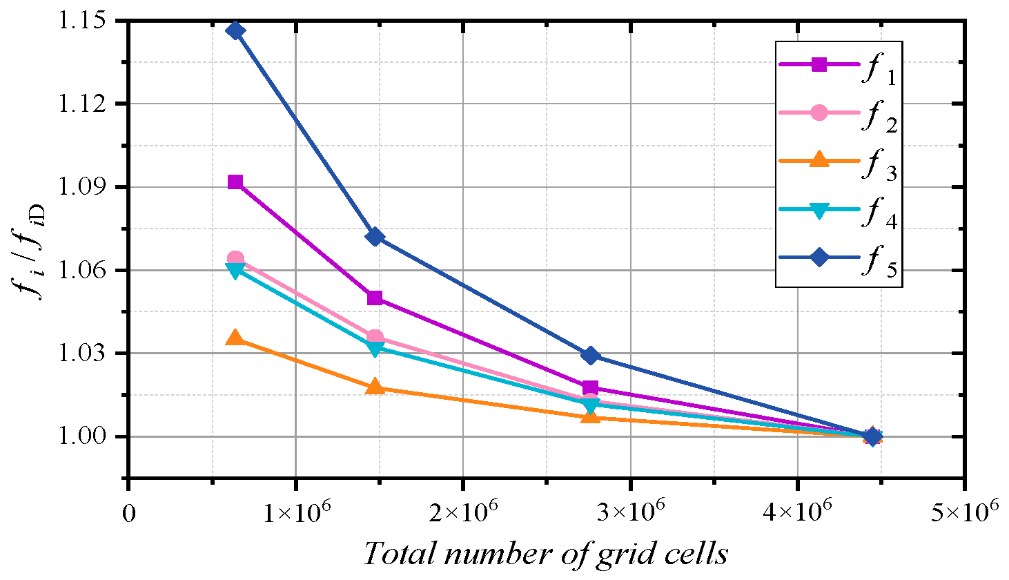
2.2. Finite Element Model

A prototype Francis pump turbine runner with nine blades was taken as the object of this article. The runner was made of structural steel: the density was 7850 kg/m3, the Poisson’s ratio was 0.3, and the elastic modulus was 200 GPa. The cut-away view and 3D modeling of the runner and the surrounding fluid are shown in Figure 1. Several geometric parameters of the runner are given here in dimensionless form.
First, the independence of the grid was checked. The fixed constraint was set at the bolt centerline, the interface between the fluid domain and the structure was set as the fluid–structure interaction surface, the interface between the fluid domain and the runner chamber was set as the rigid wall, and the interface between the fluid domain and the external fluid domain was set as the full absorption boundary.
The geometry of the clearance was very narrow; therefore, the prediction accuracy of the pressure wave could be greatly improved by using the hexahedral mesh to discretize it. However, the runner and its internal fluid were divided by tetrahedral mesh. In addition, the nodes on the fluid–structure interaction surface were kept at one-to-one correspondence. Four sets of grids were divided according to a certain proportion, named A, B, C, and D, and their parameters are shown in Table 1. For the first five modes of the runner, the frequency ratio fi/fiD was used to analyze the grid independence, and the results were shown in Figure 2. fi is the ith natural frequency of the runner, and the subscript D represents the result corresponding to the grid D.
It can be seen that the frequencies of each order tended to a stable value with the increasing number of elements. Considering the accuracy and efficiency of the solution, grid C was selected for the simulations. The finite element model is shown in Figure 3.

2.3. Definition of Vibration Mode

For hydraulic machinery runners, the vibration mode is similar to that of a disk. To describe and analyze the modes of the runner conveniently, the concepts of nodal diameter (ND) and nodal circle (NC) in the vibration mode of the disks should be introduced. ND and NC refer to the straight or circumferential line where the displacement of the disc structure remains at zero during vibration. In fact, ND and NC modes refer specifically to axial vibration. However, there are also circumferential and radial vibrations in the modes of the disk-like structure, as shown in Figure 4.
The geometry of the runner is much more complicated than that of the disk. Therefore, there are some special vibration patterns in ND and NC modes, such as crown dominant (CD), band dominant (BD), and counter phase (CP) [15]. In addition, the modes of the runner also include the vibration modes dominated by blades.

3. Results and Discussion

3.1. Modes under Different Constraints

The fixed constraints were set on the shaft-connecting surface, bolt centerline, and the top of the short shaft, respectively (as shown in Figure 1), and then the modes of the runner in channels were calculated by the acoustic–structure coupling method. The modal shapes and the natural frequencies under different constraints were compared.
The first 10 modes of the runner under surface constraint are shown in Figure 5. Among them, the first five modes are typical ND and NC modes; the sixth is the torsional mode; the seventh is the radial vibration mode; the eighth and tenth order modes are dominated by blade vibration; and the ninth is an 0NC-CP mode. The deformation of the 0NC-CP mode was concentrated at the position where the inlet edge was far away from the blade due to restriction of the blade to the upper crown and lower band.
Comparing the modes under different constraint conditions, it was found that the change of the modal shapes was generally small. The shapes of the 1ND mode, the 0NC mode, the Torsional mode, and the Radial mode changed obviously, as shown in Table 2. For the radial mode with the most obvious change, the maximum vibration point moved upward and even showed a certain axial swing when the shaft was considered.
To analyze the influence of the constraint condition on the natural frequencies, the frequency fS under surface constraint was defined as the reference value. Then, the frequency ratios fL/fS and fSh/fS were obtained by dividing the natural frequencies fL (under line constraint) and fSh (under shaft constraint) with the corresponding reference frequencies. The frequency ratio of each mode is shown in Figure 6. It can be seen that the influence of the constraints on the frequencies of different modes was quite different. Among them, the Torsional and the Radial modes were the most variable modes, especially affected by the rotating shaft. For example, the frequency of the Torsional mode was reduced to 0.851 fS under the line constraint, and the frequency could be further reduced to 0.307 fS when the shaft was considered. For the ND modes, the 1ND mode was most affected by the constraints. Additionally, with the increase in the order, the influence decreased rapidly. A similar rule also appeared in the NC modes, but it changed slowly. For the modes dominated by blade vibration, the change of the frequency with the constraint condition could be ignored.
If only the maximum difference of natural frequencies under different constraints is concerned, it can be described by Δ m = (fmaxfmin) fS. fmax and fmin are the maximum and minimum natural frequencies of a mode under different constraints. The Δ m of each mode is shown in Table 3. It can be seen that the Torsional mode, the Radial mode, the 1ND mode, and the 0NC mode varied most significantly with the constraint condition. The maximum differences in the natural frequencies of these four modes under different constraints were 69.3%, 56.4%, 35.1%, and 9.4%, respectively. When these modes are involved in practical engineering problems, it is necessary to carefully analyze whether the setting of constraint condition is reasonable, especially considering the influence of the shaft or even the rotor system. For example, if the constraint condition is not accurate, it is likely to misjudge the resonance characteristics of the runner when the 1ND exciting force appears in the unit.
Theoretically, the above results are reasonable. When the surface constraint was adopted, the local stiffness was the largest, and the natural frequencies of the runner were the highest. When the line constraint or shaft constraint was used instead, the local stiffness was reduced, and the natural frequencies were reduced. It can be seen from the modal shapes that the stiffness here strongly restricted the movement of the Torsion mode, the Radial mode, the 1ND mode, and the ONC mode, and the restriction on the movement of other modes was weak. Therefore, the change of the natural frequencies presented such a rule.

3.2. Modes Considering Energy Loss on the Wall

The rigid wall boundary on the runner chamber was changed to the absorption boundary, and the absorption coefficient α was set to 0.2, 0.4, and 0.6, respectively. Firstly, the results showed that the absorption coefficient had no impact on the shapes of most modes except the 1NC mode. When α increased to 0.2, the position of the nodal circle of the 1NC mode obviously moved outward, and the position of maximum displacement shifted from the outer edge to the center; when α increased to 0.4, the 1NC mode disappeared. The change of the modal shape was shown in Figure 7.
Figure 8 shows the variation of the natural frequency of each mode with the absorption coefficient. Here, the frequency ratio fα/f0 was used for demonstration. fα is the natural frequency under different absorption coefficients, and f0 is the frequency when the absorption coefficient is 0.
The results showed that, with the increase in the absorption coefficient on the runner chamber, the natural frequencies of the runner increased except for a few modes. It is well known that the proximity of the outer wall increases the added mass of water, thereby reducing the natural frequencies of the underwater structure. When the outer wall was not rigid, it vibrated along with the structure–water system and absorbed some of the energy in the pressure wave. At this time, the influence of the wall on the added mass was weakened, so the natural frequencies of the structure increased. Among them, the frequency change of the NC modes was the most significant, followed by the ND modes and the Torsional mode. The variation of the Radial mode and the blade vibration modes could be ignored. Compared with other modes, the frequencies of the NC modes changed too much; thus, they are shown separately in Figure 8a. For the NC modes, the change rule of the frequency of each mode was different. In particular, the frequency of the 1NC mode was abnormal. When α increased to 0.2, the frequency of the 1NC mode decreased by approximately 35%. Meanwhile, the frequencies of 0NC and 0NC-CP modes increased by 7% and 1%, respectively. For the ND modes, the change of the frequency of each mode with the absorption coefficient was almost the same. Additionally, with the increase in α, the frequency gradient of the ND modes increased.
In fact, the proximity of the wall has very different effects on the added mass of different modes. For example, during the movement of the nodal circle modes, the runner moves upward or downward as a whole to squeeze the water in the side chamber. At this time, the wall has a strong reaction force against the runner–water system, which causes a great added mass. For the blade vibration modes, the Radial mode, etc., the influence of the wall on the added mass is very small. The above results can be found in the study of Li et al. [21]. In the same way, when the absorption coefficient on the wall increased, the change in the added mass of the nodal circle modes was the most obvious, and the change in the blade vibration modes and the Radial mode was small. As for the abnormal change of the 1NC modal frequency, we think that it was caused by the change of the modal shape.
In general, the energy loss on the runner chamber had little impact on the runner’s modes. When α was increased from 0 to 0.2, the frequency variation of each mode was within 0.5%, except for the NC modes. Therefore, in the numerical modal analysis of the runner, only the influence of the energy loss on the NC modes needs to be considered.

4. Conclusions

In this paper, the influence of the constraint condition and the energy loss on the natural modes of hydraulic machinery runner was analyzed. The conclusions are as follows.
The constraint condition determines the local stiffness of the structure; therefore, it has a significant impact on the modes of the runner. The influence of constraint condition on the frequencies of the different modes is quite different, and the degree of the effect is closely related to the modal shapes. Among them, the Torsional mode, the Radial mode, the 1ND mode, and the 0NC mode varied most significantly with the constraint condition. The maximum differences in the natural frequencies of these four modes under different constraints were 69.3%, 56.4%, 35.1%, and 9.4%, respectively. When the above modes are involved in practical engineering problems, the rationality of the setting of the constraint condition must be carefully analyzed. In particular, the correct modelling of the shaft region is essential for the correct determination of natural frequencies and avoiding exciting frequencies.
When the chamber wall was not rigid, it vibrated along with the structure–water system and absorbed some of the energy in the pressure wave. At this time, the influence of the wall on the added mass was weakened, so the natural frequencies of the structure increased. The frequency variations of the Radial mode and the blade vibration modes can be ignored, and the variations of the ND modes and the Torsional mode are also small, but the variations of the NC modes are significant. Except for several specific modes, the modal shapes of the runner were almost unchanged. The results showed that it is necessary to pay attention to the influence of the energy loss on the chamber on the NC modes in the numerical modal analysis of the runner.

Author Contributions

Conceptualization, Z.W.; methodology, Z.W.; software, X.X.; validation, D.L. and J.Y.; formal analysis, D.L.; investigation, J.Y.; resources, Z.W.; writing—original draft preparation, X.X.; writing—review and editing, D.L.; funding acquisition, Z.W.; All authors have read and agreed to the published version of the manuscript.

Funding

This research was funded by the National Natural Science Foundation of China, grant number 51876099.

Institutional Review Board Statement

Not applicable.

Informed Consent Statement

Not applicable.

Data Availability Statement

Not applicable.

Conflicts of Interest

The authors declare no conflict of interest. The funders had no role in the design of the study; in the collection, analyses, or interpretation of data; in the writing of the manuscript, or in the decision to publish the results.

References

  1. Liang, Q.W.; Wang, Z.W.; Fang, Y. Modal analysis of Francis turbine with considering FSI. J. Hydroelectr. Eng. 2004, 23, 116–120. (In Chinese) [Google Scholar]
  2. Rodriguez, C.G.; Egusquiza, E.; Escaler, X.; Liang, Q.; Avellan, F. Experimental investigation of added mass effects on a Francis turbine runner in still water. J. Fluids Struct. 2006, 22, 699–712. [Google Scholar] [CrossRef]
  3. Han, Q.L.; Xing, W.T.; Li, W.H.; Zhang, Z.; Guo, S.S. Experimental modal analysis of blades in different media. Acta Energ. Sol. Sin. 2019, 40, 285–290. (In Chinese) [Google Scholar]
  4. Presas, A.; Valero, C.; Huang, X.X.; Egusquiza, E.; Farhat, M.; Avellan, F. Analysis of the dynamic response of pump-turbine runners—Part I: Experiment. In Proceedings of the IOP Conference Series: Earth and Environmental Science, Beijing, China, 19–23 August 2012; IOP Publishing: Bristol, UK, 2012; Volume 15. [Google Scholar]
  5. Østby, P.T.K.; Sivertsen, K.; Billdal, J.T.; Haugen, B. Experimental investigation on the effect off near walls on the eigen frequency of a low specific speed francis runner. Mech. Syst. Signal Process. 2019, 118, 757–766. [Google Scholar] [CrossRef]
  6. Egusquiza, E.; Valero, C.; Liang, Q.W.; Coussirat, M.; Seidel, U. Fluid added mass effect in the modal response of a pump-turbine impeller. In Proceedings of the 2009 International Conference on Mechatronic and Embedded Systems and Applications, San Diego, CA, USA, 30 August–2 September 2009; Volume 48982, pp. 715–724. [Google Scholar]
  7. Hübner, B.; Seidel, U.; Roth, S. Application of fluid-structure coupling to predict the dynamic behavior of turbine components. In Proceedings of the 25th IAHR Symposium on Hydraulic Machinery and Systems, Timisoara, Romania, 20–24 September 2010. [Google Scholar]
  8. Liu, X.; Luo, Y.Y.; Karney, B.W.; Wang, Z.; Zhai, L. Virtual testing for modal and damping ratio identification of submerged structures using the PolyMAX algorithm with two-way fluid-structure Interactions. J. Fluids Struct. 2015, 54, 548–565. [Google Scholar] [CrossRef]
  9. Liang, Q.W.; Rodriguez, C.G.; Egusquiza, E.; Escaler, X.; Farhat, M.; Avellan, F. Numerical simulation of fluid added mass effect on a francis turbine runner. Comput. Fluids 2007, 36, 1106–1118. [Google Scholar] [CrossRef]
  10. Egusquiza, E.; Valero, C.; Huang, X.X.; ou, E.; Guardo, A.; Rodriguez, C. Failure investigation of a large pump-turbine runner. Eng. Fail. Anal. 2012, 23, 27–34. [Google Scholar] [CrossRef] [Green Version]
  11. Huang, X.X.; Escaler, X. Added mass effects on a Francis turbine runner with attached blade cavitation. Fluids 2019, 4, 107. [Google Scholar] [CrossRef] [Green Version]
  12. Huang, X.X.; Oram, C.; Sick, M. Static and dynamic stress analyses of the prototype high head Francis runner based on site measurement. In Proceedings of the IOP Conference Series: Earth and Environmental Science, Montreal, QC, Canada, 22–26 September 2014; IOP Publishing: Bristol, UK, 2014; Volume 22, p. 032052. [Google Scholar]
  13. Rodriguez, C.G.; Flores, P.; Pierart, F.G.; Contzen, L.R.; Egusquiza, E. Capability of structural-acoustical FSI numerical model to predict natural frequencies of submerged structures with nearby rigid surfaces. Comput. Fluids 2012, 64, 117–126. [Google Scholar] [CrossRef]
  14. Askari, E.; Jeong, K.; Amabili, M. Hydroelastic vibration of circular plates immersed in a liquid-filled container with free surface. J. Sound Vib. 2013, 332, 3064–3085. [Google Scholar] [CrossRef]
  15. He, L.Y.; Zhou, L.J.; Ahn, S.H.; Wang, Z.; Nakahara, Y.; Kurosawa, S. Evaluation of gap influence on the dynamic response behavior of pump-turbine runner. Eng. Comput. 2019, 36, 491–508. [Google Scholar] [CrossRef]
  16. Valentín, D.; Ramos, D.; Bossio, M.; Presas, A.; Egusquiza, E.; Valero, C. Influence of the boundary conditions on the natural frequencies of a Francis turbine. In Proceedings of the IOP Conference Series: Earth and Environmental Science, Grenoble, France, 4–8 July 2016; IOP Publishing: Bristol, UK, 2016; Volume 49, p. 072004. [Google Scholar]
  17. Egusquiza, E.; Valero, C.; Presas, A.; Huang, X.; Guardo, A.; Seidel, U. Analysis of the dynamic response of pump-turbine impellers. Influence of the rotor. Mech. Syst. Signal Process. 2016, 68, 330–341. [Google Scholar] [CrossRef]
  18. Woyjak, D.B. Acoustic and Fluid Structure Interaction, A Revision 5.0 Tutorial; Swanson Analysis Systems: Houston, TX, USA, 1992. [Google Scholar]
  19. Rajakumar, C.; Ali, A. Acoustic boundary element eigenproblem with sound absorption and its solution using lanczos algorithm. Int. J. Numer. Methods Eng. 1993, 36, 3957–3972. [Google Scholar] [CrossRef]
  20. ANSYS Inc. Mechanical APDL Theory Guide; ANSYS: Canonsburg, PA, USA, 2017. [Google Scholar]
  21. Li, D.K.; Xia, X.; Zhou, L.J.; Gong, K.; Wang, Z. Effect of outer edge modification on dynamic characteristics of pump turbine runner. Eng. Fail. Anal. 2021, 124, 105379. [Google Scholar] [CrossRef]
Figure 1. Schematic diagram of the runner and surrounding fluid.
Jmse 09 00434 g001
Figure 2. The first five natural frequencies of the runner in channels with different grid sizes.
Jmse 09 00434 g002
Figure 3. Finite element model of fluid–structure coupling modal analysis of runner.
Jmse 09 00434 g003
Figure 4. Schematic of vibration modes of a disk.
Jmse 09 00434 g004
Figure 5. The first 10 modes of the runner with surface constraint.
Jmse 09 00434 g005
Figure 6. Influence of the constraint condition on the natural frequencies.
Jmse 09 00434 g006
Figure 7. Variation of the 1NC mode with absorption coefficients.
Jmse 09 00434 g007
Figure 8. Variation of the natural frequencies with absorption boundary: (a) NC modes; (b) other modes.
Jmse 09 00434 g008
Table 1. Grid parameters of fluid structure coupling modal analysis of runner.
GridABCD
Unit number of structure (-)271,271638,7131,209,7952,033,087
Unit number of water (-)366,915834,0531,551,4372,414,909
Total unit number (-)638,1861,472,7662,761,2324,447,996
Table 2. Modal shapes under different constraints.
1ND0NCTorsionalRadial
Surface constraint Jmse 09 00434 i001 Jmse 09 00434 i002 Jmse 09 00434 i003 Jmse 09 00434 i004
line constraint Jmse 09 00434 i005 Jmse 09 00434 i006 Jmse 09 00434 i007 Jmse 09 00434 i008
shaft constraint Jmse 09 00434 i009 Jmse 09 00434 i010 Jmse 09 00434 i011 Jmse 09 00434 i012
Table 3. Maximum differences of natural frequencies under different constraints.
Modal1ND2ND3ND0NC1NC
Δ m 0.3510.0170.0040.0940.027
Modal0NC-CPTorsionalRadialBlade IBlade II
Δ m 0.0160.6930.5640.0030.011
Publisher’s Note: MDPI stays neutral with regard to jurisdictional claims in published maps and institutional affiliations.

