Article

High-Frequency Radar Cross Section of Ocean Surface for an FMICW Source

1
The School of Information Engineering, Nanchang University, Nanchang 330031, China
2
The School of Electronic Information, Wuhan University, Wuhan 430072, China
*
Authors to whom correspondence should be addressed.
J. Mar. Sci. Eng. 2021, 9(4), 427; https://doi.org/10.3390/jmse9040427
Submission received: 23 March 2021 / Revised: 10 April 2021 / Accepted: 12 April 2021 / Published: 15 April 2021
(This article belongs to the Special Issue Development of Oceanographic Sensors)

Abstract

:
The frequency-modulated interrupted continuous waveform (FMICW) has been widely used in remotely sensing sea surface states by high-frequency ground wave radar (HFGWR). However, the radar cross section model of the sea surface for this waveform has not yet been presented. Therefore, the first- and second-order cross section models of the sea surface about this waveform are derived in this study. The derivation begins with the general electric field equations. Subsequently, the FMICW source is introduced as the radar transmitted signal to obtain the FMICW-incorporated backscattered electric field equations. These equations are used to calculate range spectra by Fourier transforming. Therefore, Fourier transformation of the range spectra calculated from successive sweep intervals gives the Doppler spectra or the power spectral densities. The radar cross section model is obtained by directly comparing the Doppler spectra with the standard radar range equation. Moreover, the derived first- and second-order radar cross section models for an FMICW source are simulated and compared with those for a frequency-modulated continuous waveform (FMCW) source. Results show that the cross section models for the FMICW and FMCW cases have different analytical expressions but almost the same numerical results.

1. Introduction

High-frequency ground wave radar (HFGWR) can be used to monitor ocean surface sea states with high spatial and temporal resolution [1,2,3]. The working frequency of the HFGWR is in the high-frequency (HF) band (3–30 MHz). Radio signals within this frequency band strongly interact with the ocean surface waves [4]. Moreover, these radio signals can propagate along the ocean surface to ranges well beyond 200 km due to the high conductivity of the ocean water [5]. The backscattered signals contain significant information about the ocean surface sea states [6]. To extract the sea states from the backscattered signals, a scatter model or cross section model of the ocean surface for the HFGWR is crucial theoretical basis.
So far, the derivation of the HFGWR cross section model of the ocean surface has been studied for over four decades. Seminal studies by Barrick [7] first presented a HFGWR cross section model. Later, Walsh and his colleagues addressed the cross section model based on a generalized function theory with the assumption of a dipole source [8,9]. This approach also has been extended to develop models for some complex scenes, such as bistatic HFGWR system [10,11], receiving and transmitting antennas on a floating platform [12,13], an antenna on a floating platform for bistatic HFGWR system [14,15], and shipborne HFGWR system [16]. All of these models are developed specifically for pulsed waveform HFGWR. However, in pulsed radar system, the competing relationship between range resolution and detectable range results in a trade-off between achieving long range and increasing range resolution. Compared to this, frequency-modulated continuous waveform (FMCW) radar can achieve high range resolution and long detection range, as the FMCW has a 100% duty cycle and its bandwidth can be configured freely. Consequently, FMCW has been widely used in HFGWR and the corresponding cross section models also have been studied. Walsh et al. [17] presented the first- and second-order monostatic radar ocean surface cross sections for an FMCW source. Furthermore, a bistatic HFGWR ocean surface cross section model for an FMCW source with an antenna on a floating platform has been established and simulated [18]. Moreover, the FMCW HFGWR cross section model for mixed-path ionosphere–ocean propagation has been developed in [19]. However, when the transmitter and receiver are collocated, the transmitted FMCW signal will overwhelm the HFGWR receiver due to the simultaneous running of the transmitter and receiver. Thus, a frequency-modulated interrupted continuous waveform (FMICW), which consists of a gating signal and an FMCW signal, has been designed for HFGWR to handle this problem [20]. Just like the FMCW, such FMICW can also provide high sensitivity, range, and Doppler information, and avoid aliasing and ambiguities. Because of these characteristics, the FMICW has been widely used throughout the HFGWR remote sensing community. However, the HFGWR cross section model for ocean surface about the FMICW source has not yet been presented.
In this paper, we derive the HFGWR cross section model of the ocean surface for the FMICW source. In Section 2, the electric field equations related to the FMICW source are first deduced, and the power spectral density (PSD) of the received electric field is obtained. Then, the first- and second-order cross section models are also derived in this section. Section 3 provides simulation and discussion about the derived cross section model. Section 4 gives a summary of the paper.

2. Derivation of the Cross Section

2.1. General First- and Second-Order Electric Field Equations

For a general vertically polarized HF source, the general equations for the scattered electric field from rough sea surface have been developed by Walsh and Gill [9]. The first-order scattered electric field for a monostatic radar in frequency domain, E 1 ( ω ) , can be written as
E 1 ( ω ) = k C 0 ( 2 π ) 3 / 2 K P K K ρ F 2 ( ρ ) ρ 3 / 2 e j π / 4 e j ρ ( K 2 k ) d ρ
Here, C 0 = Δ l k 2 I ( ω ) j ω ϵ 0 is the dipole constant for a dipole of length Δ l carrying a current I ( ω ) whose radian frequency is ω and whose wave number is k in a space with permittivity of ϵ 0 . P K denotes the Fourier coefficient of the scattering surface whose wave vector is K with a magnitude of K and a direction of θ K (i.e., K = ( K , θ K ) ). ρ represents the distance between the radar and the scattering patch. F ( ρ ) is the Sommerfeld attenuation function. Correspondingly, the second-order scattered electric field for a monostatic radar, E 2 ( ω ) , can be expressed as
E 2 ( ω ) = k C 0 ( 2 π ) 3 / 2 K 1 K 2 P K 1 P K 2 K S Γ P × ρ F 2 ( ρ ) ρ 3 / 2 e j π / 4 e j ρ ( K 2 k ) d ρ
This expression accounts for the total electric field originating from a single scatter from second-order ocean waves and a twice scatter by a rough patch surface. K 1 and K 2 are the two first-order ocean wave vectors forming a second-order ocean wave for the single scatter case and are the first and second scattering wave vectors for the twice scatter case. These two wave vectors satisfy the constraint K 1 + K 2 = K in these two cases. P K 1 and P K 2 are the Fourier coefficients associated with K 1 and K 2 , respectively. S Γ P is the total coupling coefficient, which is defined as S Γ P = E Γ P H Γ P , where E Γ P and H Γ P , respectively, are the electromagnetic coupling coefficient and the hydrodynamic coupling coefficient.
Here, both Equations (1) and (2) are different from their counterparts presented in Walsh and Gill [9]. The term containing factors of e j π / 4 e j ρ ( K + 2 k ) has been omitted from the integrals in both Equations (1) and (2). Moreover, the antenna gain has been replaced with constant 1. However, Equation (1) is exactly the same as Equation (6) in Walsh et al. [17]. Equation (2) is derived from the analysis in Walsh and Gill [11] and also consisting with the equations in Walsh et al. [17].

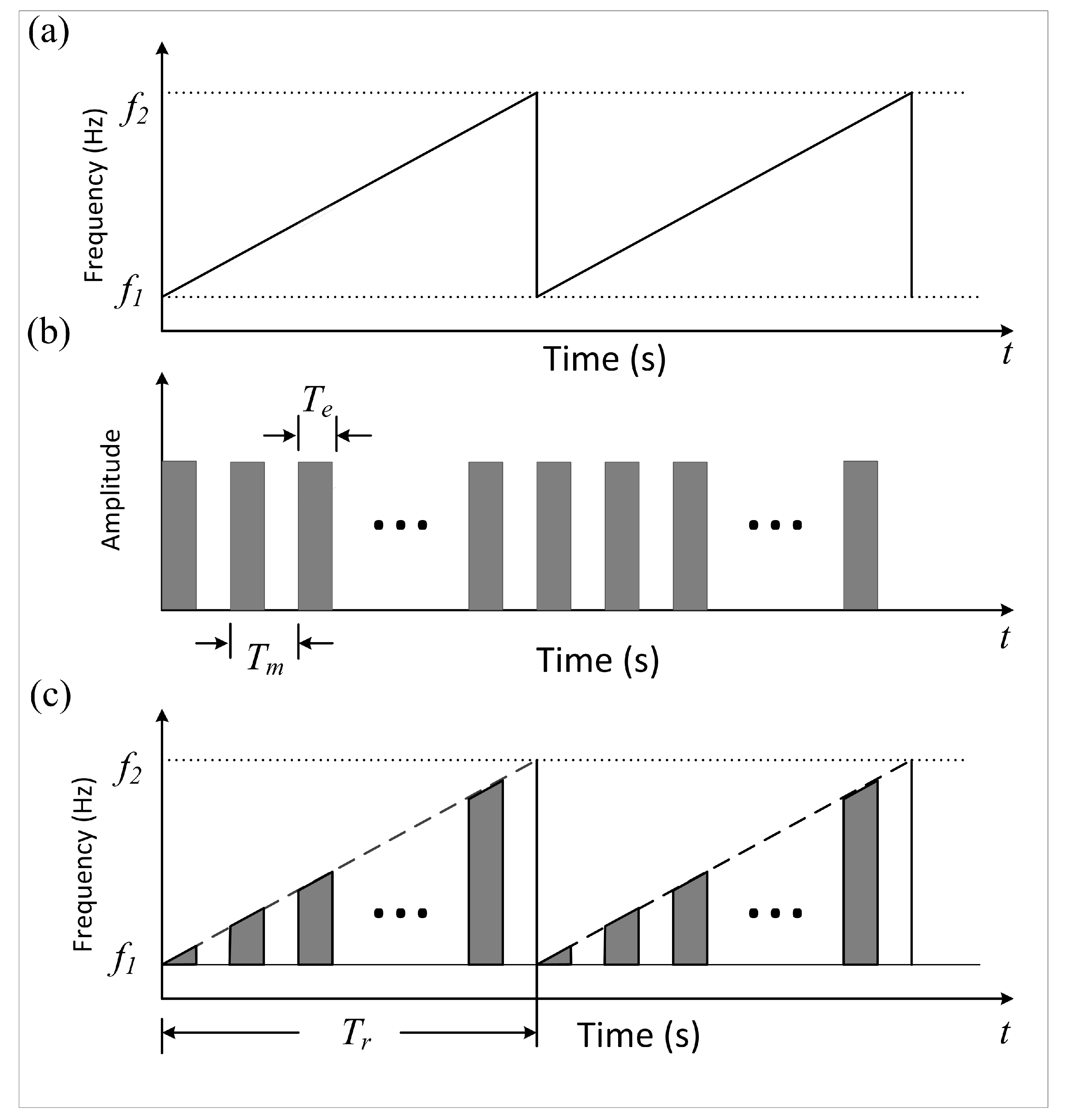
2.2. The FMICW Source

A typical example of an FMICW signal is shown in Figure 1. The FMICW can be treated as an FMCW times a gate function. The FMCW signal, c ( t ) , in this study, only the up-sweep is considered. Therefore, c ( t ) for one sweep interval can be given as
c ( t ) = I 0 e j ω 0 t + α π t 2 h t + T r 2 h t T r 2
where I 0 is the peak current, ω 0 is the center radian frequency, α is the frequency sweep rate, and h is the usual Heaviside function. Referring to Figure 1, we have ω 0 = ( f 2 + f 1 ) × π and α = ( f 2 f 1 ) / T r . Besides, the gate function, g ( t ) , within one sweep interval ( T r ) can be expressed as
g ( t ) = n = 0 N 1 h t + T r 2 n T m h t + T r 2 n T m T e
where N = T r / T m represents the number of periods of the gate function within one sweep. Thus, the FMICW signal, i ( t ) , within one sweep interval can be cast as
i ( t ) = c ( t ) · g ( t ) = I 0 e j ω 0 t + α π t 2 n = 0 N 1 h t + T r 2 n T m h t + T r 2 n T m T e

2.3. Electric Field Equations Incorporating the FMICW Source

Following a similar analysis as in [17,18,19], Equation (1) can be inversely Fourier-transformed to give the received electric field in the time domain as
E 1 ( t ) = F 1 E 1 ( ω ) = 1 ( 2 π ) 3 / 2 K P K K ρ F 2 ρ ρ 3 / 2 e j K ρ F 1 k C 0 · e j 2 k ρ e j π / 4 d ρ
where F 1 represents the inverse Fourier transformation. The transformation in this equation can be expressed as
F 1 k C 0 · e j 2 k ρ = F t 1 k C 0 · e j 2 ω ρ / c = F t 1 k C 0 * t δ t 2 ρ c
where * t indicates a time convolution and δ ( · ) is the Dirac delta function. Using c = 1 / μ 0 ϵ 0 , where μ 0 is permeability of the free space, η 0 = μ 0 / ϵ 0 , and the FMICW source in Equation (5), the inverse Fourier transform of k C 0 is given by
F 1 k C 0 = j η 0 Δ l c 2 2 i ( t ) t 2 j I 0 η 0 Δ l ω 0 2 c 2 e j ω 0 t + α π t 2 × n = 0 N 1 h t + T r 2 n T m h t + T r 2 n T m T e
Here, the leading and trailing edge impulse terms in the derivative of Equation (5) are neglected. Similar neglect is extensively used in related open literature, such as in [17,18,19,21]. Besides, the approximation in Equation (8) is permissible because ω 0 2 π α t . Using Equations (7) and (8) in Equation (6), we can obtain
E 1 t r = j I 0 η 0 Δ l k 0 2 ( 2 π ) 3 2 K P K K e j π 4 × 0 F 2 ρ ρ 3 2 e j ω 0 t r + α π t r 2 e j K 2 k 0 ρ e j 4 π α ρ c t r e j 4 π α ρ 2 c 2 × n = 0 N 1 h t r + T r 2 2 ρ c n T m h t r + T r 2 2 ρ c n T m T e d ρ
where k 0 = ω 0 / c , and t has been renamed to t r for emphasizing that the time is within the interval of T r / 2 , T r / 2 .
At this stage, the received electric field signal is demodulated for further processing. This demodulation involves coherently mixing the acquired signal with an FMCW signal, which contains the same linear frequency ramp with the transmitted original FMICW signal (details can be found in [20]), and low-pass filtering the outcome. Consequently, the factor involving e j ω 0 t r + α π t r 2 will be eliminated, the phase terms will be replaced by their complex conjugate, and the other factors remain the same. Equation (9) becomes
E 1 D t r = j I 0 η 0 Δ l k 0 2 ( 2 π ) 3 2 K P K K e j π 4 × 0 F 2 ρ ρ 3 2 e j K 2 k 0 ρ e j 4 π α ρ 2 c 2 e j 4 π α ρ c t r × n = 0 N 1 h t r + T r 2 2 ρ c n T m h t r + T r 2 2 ρ c n T m T e d ρ
where E 1 D t r represents the demodulated version of E 1 t r .
The next step within the process is to Fourier transform the demodulated electric field with respect to t r to obtain the so-called “range transform”, which is denoted as E 1 D ( ω r ) with ω r being the frequency variable. On the other hand, in Equation (10), only the last two terms are a function of t r . Therefore, the Fourier transformation only performs on the last two terms to obtain E 1 D ( ω r ) , which is given as
E 1 D ( ω r ) = j I 0 η 0 Δ l k 0 2 T e ( 2 π ) 3 / 2 K P K K e j π 4 ρ F 2 ( ρ ) ρ 3 / 2 e j ( K 2 k 0 + 2 k r ) ρ e j 4 π α c 2 ρ 2 × n = 0 N 1 e j ( 4 π α ρ c ω r ) ( n T m + T e 2 T r 2 ) S a T e 2 ω r 4 π α ρ c d ρ
where S a ( x ) = sin x / x and k r = ω r / c . Defining a range ρ r as ρ r = c ω r 4 π α and a range variable ρ s as ρ s = ρ ρ r , we have d ρ = d ρ s and
E 1 D ( ω r ) = j I 0 η 0 Δ l k 0 2 T e ( 2 π ) 3 / 2 K P K K e j π 4 e j K 2 k 0 + k r ρ r ρ s F 2 ρ r + ρ s ρ r + ρ s 3 / 2 × e j K 2 k 0 ρ s e j k r ρ s 2 / ρ r e j k e k B ρ s × n = 0 N 1 e j ω r n T m ρ s / ρ r S a k e ρ s d ρ s .
where k e = 2 π α T e / c and k B = 2 π α T r / c . We also should note that
n = 0 N 1 e j ω r n T m ρ s / ρ r = e j N 1 N k B ρ s sin ( k B ρ s ) sin ( 1 N k B ρ s ) .
Here, the factor sin ( k B ρ s ) sin ( k B ρ s / N ) performs a “band-pass” sampling of the variable ρ s , which obviously is similar to a beam pattern formed from a uniform linear antenna array in sampling bearing domain. Consequently, most of the return is from the values of ρ s = 0 within the main lobe of this sampling factor. In other words, the most of the contribution to the integral about ρ s in Equation (12) should come from ranges in a neighborhood of the peak ( ρ s = 0 , ρ = ρ r ) . One way to stipulate this is to specify the values of ρ s as
π 2 < k B ρ s < π 2 π 2 k B < ρ s < π 2 k B
Therefore, a convenient and common definition of range resolution ( Δ ρ ) can be expressed as
Δ ρ = 2 π 2 k B = c 2 B
where B = α T r . On the other hand, in the physical sense, it can be assumed that ρ r Δ ρ / 2 . This will be true generally when the scattering patch is a few kilometers from the radar. Besides, it has been proved that the factor containing the exponent of ρ s 2 in Equation (12) can be neglected as small in [17]. Thus, Equation (12) can be written as
E 1 D ( ω r ) j I 0 η 0 Δ l k 0 2 T e ( 2 π ) 3 / 2 K P K K e j π 4 e j K 2 k 0 + k r ρ r F 2 ρ r ρ r 3 / 2 × Δ ρ / 2 Δ ρ / 2 e j K 2 k 0 ρ s e j k e k B ρ s × n = 0 N 1 e j ω r n T m ρ s / ρ r S a k e ρ s d ρ s = j c I 0 η 0 Δ l k 0 2 F 2 ρ r 2 α ( 2 π ρ r ) 3 / 2 K P K K e j π 4 e j K 2 k 0 + k r ρ r × n = 0 N 1 S m ( K , k e , k B , n , Δ ρ )
where S m ( K , k e , k B , n , Δ ρ ) is defined as
S m ( K , k e , k B , n , Δ ρ ) = 1 π S i K 2 k 0 + k B n ω r T m / ρ r Δ ρ 2 S i K 2 k 0 + k B n ω r T m / ρ r 2 k e Δ ρ 2 ,
and the S i is the sine integral
S i ( x ) = 0 x sin ( t ) t d t .
By direct comparison with the corresponding first-order backscatter analysis, the second-order field appearing in Equation (2) becomes
E 2 D ( ω r ) = j c I 0 η 0 Δ l k 0 2 F 2 ρ r 2 α ( 2 π ρ r ) 3 / 2 K 1 K 2 P K 1 P K 2 S Γ P × K e j π 4 e j K 2 k 0 + k r ρ r × n = 0 N 1 S m ( K , k e , k B , n , Δ ρ )

2.4. Cross Section for the FMICW Source

It is assumed that the scattered fields from successive sweeps (chirps) are collected and the scattering surface has a slow time variation. To account for this, a factor, e j ω t , should be introduced into the representations of the first- and second-order electric field equations. Consequently, we have 0cm0cm
E 1 ( ω r , t ) = j c I 0 η 0 Δ l k 0 2 F 2 ρ r 2 α ( 2 π ρ r ) 3 / 2 K P K K e j π 4 e j K 2 k 0 + k r ρ r e j ω t × n = 0 N 1 S m ( K , k e , k B , n , Δ ρ )
and
E 2 ( ω r , t ) = j c I 0 η 0 Δ l k 0 2 F 2 ρ r 2 α ( 2 π ρ r ) 3 / 2 K 1 K 2 P K 1 P K 2 S Γ P × K e j π 4 e j K 2 k 0 + k r ρ r e j ω t × n = 0 N 1 S m ( K , k e , k B , n , Δ ρ ) .
Note that the variable t in here is the sweep-to-sweep time, and it is different from the t in Section 2.2 and Section 2.3.
An approach similar to that in [11,17,18,19] is used to derive the cross section from the received electric field equations. The approach first calculates the autocorrelation functions of the electric field equations. Then, it performs Fourier transformation on the autocorrelation functions to obtain power spectral density (PSD). Finally, it derives the cross section models from comparing the normalized PSD with the standard radar range equation.
The autocorrelation function, R ( τ ) , is defined as [17]
R ( τ ) = A r 2 η 0 1 ( N T e ) 2 E ( t + τ ) E * ( t )
where τ is time shift, · denotes statistical or ensemble average, * represents complex conjugation, and A r refers to the effective aperture of the receiving antenna. Substituting Equation (20) into this definition, we have 0cm0cm
R 1 ( τ ) = A r η 0 I 0 2 Δ l 2 k 0 4 F 4 ρ r Δ ρ 2 T r 2 2 N 2 T e 2 ( 2 π ρ r ) 3 × K P K K P K * K K e j K 2 k 0 + k r ρ r e j K 2 k 0 + k r ρ r × e j ω ( t + τ ) e j ω t n = 0 N 1 S m ( K , k e , k B , n , Δ ρ ) n = 0 N 1 S m ( K , k e , k B , n , Δ ρ ) = A r η 0 I 0 2 Δ l 2 k 0 4 F 4 ρ r Δ ρ 2 T r 2 4 N 2 T e 2 ( π ρ r ) 3 × m = ± 1 π π 0 S ( m K ) e j m g K τ K 2 n = 0 N 1 S m ( K , k e , k B , n , Δ ρ ) 2 d K d θ K
Here, g is gravitational acceleration, and S ( m K ) is the directional ocean wave spectrum for wave vectors m K , with m = ± 1 .
Now, the first-order PSD P 1 ( ω d ) can be derived from the Fourier transformation; that is, P 1 ( ω d ) = F [ R 1 ( τ ) ] , where ω d is the Doppler frequency. After operating the Fourier transformation, we have
P 1 ( ω d ) = A r η 0 I 0 2 Δ l 2 k 0 4 F 4 ρ r Δ ρ 2 T r 2 8 N 2 T e 2 g π 2 ρ r 3 × m = ± 1 π π S ( m K ) K 2.5 n = 0 N 1 S m ( K , k e , k B , n , Δ ρ ) 2 d θ K
This equation accounts for the first-order electric field returns scattered by a range cell that is dictated by a width or range resolution Δ ρ at range ρ r . Therefore, the scattering area normalized first-order PSD, P 1 N ( ω d ) , can be expressed as
P 1 N ( ω d ) = P 1 ( ω d ) π π ρ r Δ ρ d θ K = A r η 0 I 0 2 Δ l 2 k 0 4 F 4 ρ r Δ ρ T r 2 8 N 2 T e 2 g π 2 ρ r 4 × m = ± 1 S ( m K ) K 2.5 n = 0 N 1 S m ( K , k e , k B , n , Δ ρ ) 2
On the other hand, the standard monostatic radar range equation takes the form
P 1 S ( ω d ) = η 0 I 0 2 Δ l 2 k 0 2 A r F 4 ρ r Δ ρ 2 ( 4 π ) 3 ρ r 4 σ 1 ( ω d )
where σ 1 ( ω d ) is the first-order cross section. Thus, direct comparison of Equation (26) with Equation (25) gives the first-order cross section for the FMICW source as
σ 1 ( ω d ) = 16 π k 0 2 T r 2 N 2 T e 2 m = ± 1 S ( m K ) K 2.5 g 1 / 2 Δ ρ n = 0 N 1 S m ( K , k e , k B , n , Δ ρ ) 2
where ω d = m g K , and the direction of the wave vector K is the radar look angle.
Similarly, using Equation (21) in Equation (22), we can obtain the autocorrelation function for second-order electric field. Then, we perform Fourier transformation to calculate PSD. By comparing the scattering-area normalized PSD with radar equation, the resulting second-order cross section for the FMICW source is
σ 2 ω d = 8 π k 0 2 T r 2 N 2 T e 2 m 1 = ± 1 m 2 = ± 1 0 π π 0 × S ( m 1 K 1 ) S ( m 2 K 2 ) S Γ P 2 K 1 K 2 Δ ρ × δ ω d + m 1 g K 1 + m 2 g K 2 × n = 0 N 1 S m ( K , k e , k B , n , Δ ρ ) 2 d K 1 d θ K 1 d K
Here, θ K 1 is the direction of K 1 , and the four possible combinations of m 1 and m 2 correspond to four different Doppler frequency regions [22].

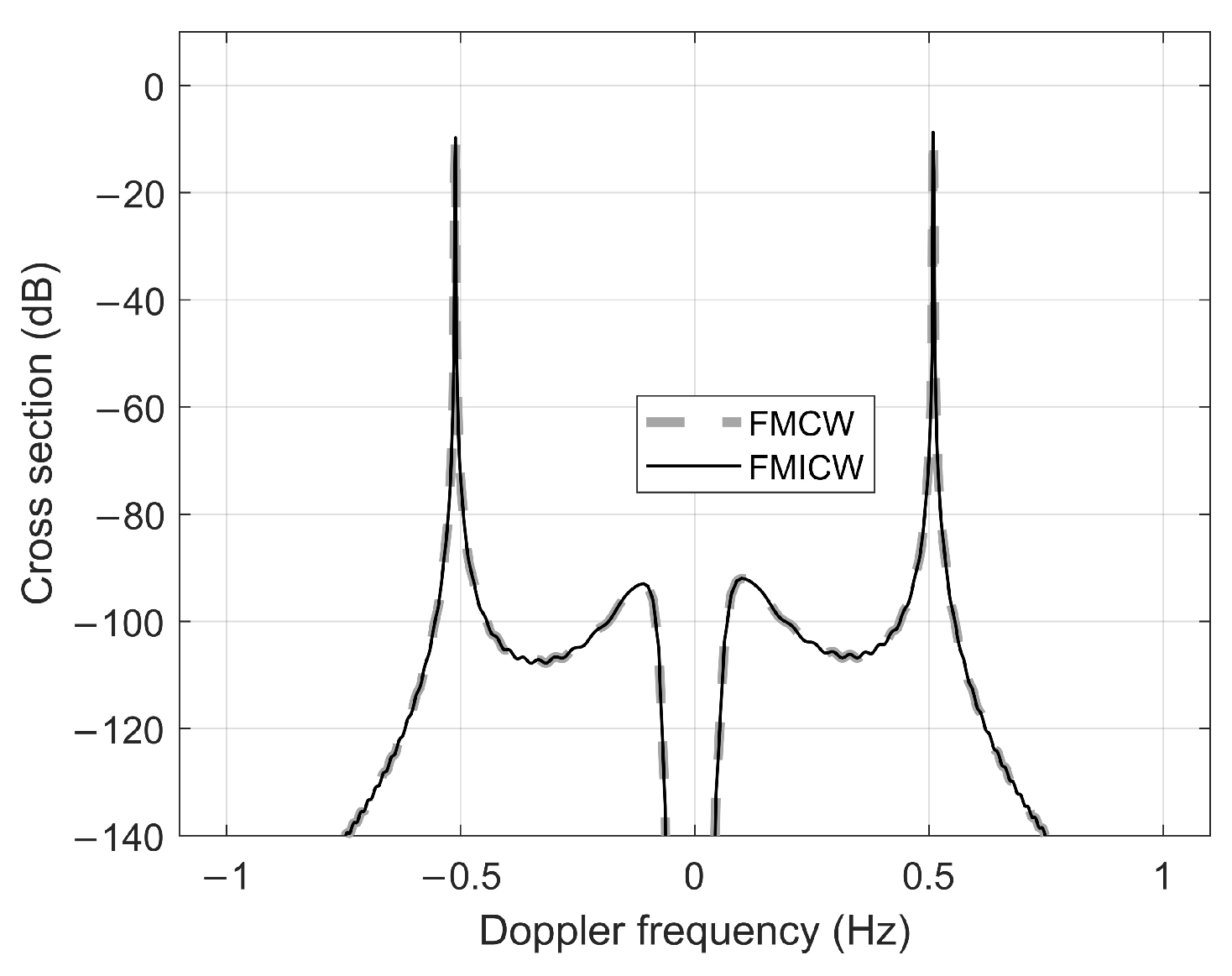
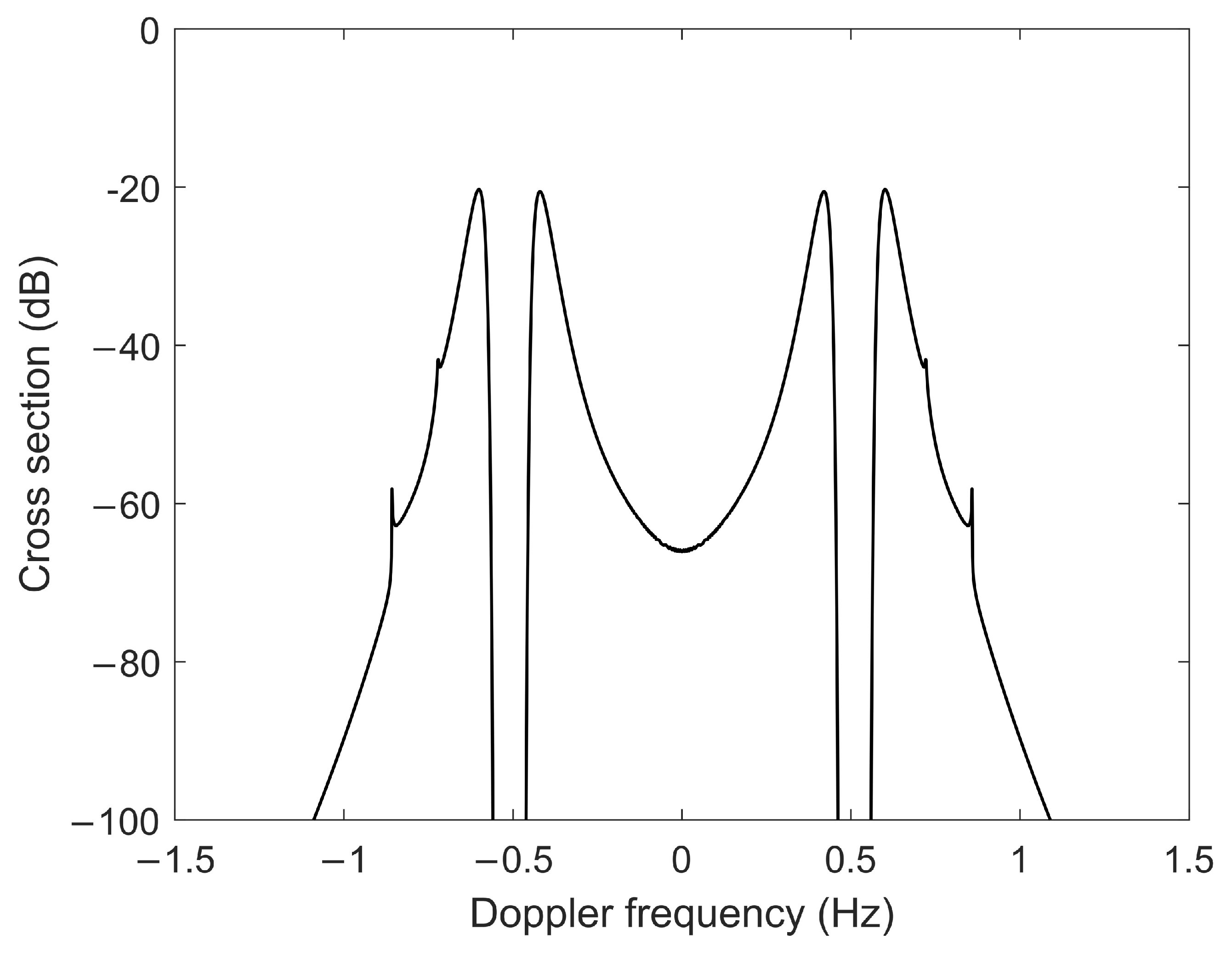
3. Simulation Results and Discussion

To illustrate the newly derived models, the radar cross section was calculated based on Equations (27) and (28). Moreover, we also intend to illustrate the differences in the cross section between the FMICW and FMCW [17] source cases. To calculate the radar cross section, a Pierson–Moskowitz (PM) ocean wave spectral model [23] with a cardioid directional spreading function was selected, as this model only needs the sea surface wind information.
Figure 2 illustrates the smoothed versions of the first-order cross section for the FMCW and FMICW sources when the central operating frequency is 25 MHz. The sweep interval, T r , is chosen as 0.39 min with the sweep bandwidth of 100 kHz. Accordingly, the corresponding range resolution, Δ ρ , is 1.5 km. The wind speed in this simulation is 15 m/s with a direction perpendicular to the radar look direction. These parameters are shared for these two waveform cases, but T e and T m are extra set for FMICW source. T e and T m are, respectively, set as 0.2 ms and 0.6 ms in this simulation.
From Figure 2, we can see that there are two narrow and sharp peaks at ± 2 g k 0 , which are classically referred to as the Bragg frequencies [7]. These two peaks, which are indicative of scatter from two ocean waves with one traveling toward and the other traveling away from radar, are the usual first-order peaks in the radar received sea echoes, and they are first experimentally observed by Crombie [4]. Note that the cross section displayed in Figure 2 is symmetrical about zero Doppler frequency, but this is not always the case. When the wind direction is not perpendicular to the radar look direction, this symmetry will not occur. Actually, the asymmetry cases have been discussed in [17], where first-order cross sections for FMCW waveform case with wind directions of 60 , 30 , and 0 relative to the radar look direction have been discussed. Besides, the effect of the sea surface currents on the first-order cross section was not taken into consideration in this study. Fortunately, existing literature has studied the effect of the sea surface currents. The sea surface currents result in Doppler frequency shifts of these two first-order peaks, and they have no effect on the amplitude [22]. These Doppler frequency shifts resulting from sea surface currents have been well modeled and used to extract ocean surface current velocity. On the other hand, Figure 2 also shows that the cross sections for the FMCW and FMICW waveforms are almost the same. According to the work in [17], the first-order cross section for the FMCW waveform is
σ 1 F M C W ( ω d ) = 16 π k 0 2 m = ± 1 S ( m K ) K 2.5 g 1 / 2 Δ ρ S m 2 ( K , k B , Δ ρ )
where k 0 , K , K, g, Δ ρ , and k B are defined in Section 2; S m ( K , k B , Δ ρ ) is defined as
S m ( K , k B , Δ ρ ) = 1 π S i ( K 2 k 0 + k B ) Δ ρ 2 S i ( K 2 k 0 k B ) Δ ρ 2
with S i ( · ) defined in Equation (18). Comparing Equation (27) with Equation (29) suggests that these two models are obviously different. However, these two models are numerically almost the same. It is verified numerically that the intrinsic cause for the cross sections of these two waveforms to be almost numerically identical is
S m 2 ( K , k B , Δ ρ ) T r 2 N 2 T e 2 × n = 0 N 1 S m ( K , k e , k B , n , Δ ρ ) 2 .
On the other hand, note that the FMCW is a special case for the FMICW with a duty cycle of 100 percent. Thus, the cross section model for the FMICW implicitly includes the FMCW cross section case. It is easily known that Equation (27) can be simplified to Equation (29) for the case of T e = T m , which is just the FMCW source case.
Just like the first-order cross section model, the difference between the second-order cross section models for the FMCW source and the FMICW source also is S m 2 ( K , k B , Δ ρ ) being replaced with T r 2 N 2 T e 2 × n = 0 N 1 S m ( K , k e , k B , n , Δ ρ ) 2 . This difference can be easily verified from comparing Equation (28) with the FMCW model in [17]. Considering Equation (31), we can infer that the second-order cross sections for FMCW and FMICW cases are numerically almost the same.
To simulate the second-order cross section for the FMICW source, a similar technique used in [11,17] was adopted. Figure 3 illustrates the second-order cross section calculated from Equation (28) with all the waveform and sea states (or wind) parameters being the same as the before-mentioned first-order cross section displayed in Figure 2. Figure 3 illustrates that there are relative maxima of the second-order cross section adjacent to the positive and negative Bragg frequencies (±0.51 Hz). These maxima result from the fact that ω d being very close to ± 2 g k 0 will lead to K 1 or K 2 nearing zero. On the contrary, ω d being far away from ± 2 g k 0 will result in K 1 or K 2 being a large value. In the PM ocean wave spectral model, both large and small wave numbers have a low spectral energy, which leads to the term S ( m 1 K 1 ) S ( m 2 K 2 ) in Equation (28) being small, while medium wave numbers have relative large spectral energy, meaning that S ( m 1 K 1 ) S ( m 2 K 2 ) has a relative large value. Moreover, there are local peaks at frequency positions of ± 0.721 and ± 0.858 . These frequency positions are equal to the theoretical singular peaks at ± 2 g k 0 and the “corner reflector” peaks at ± 2 3 / 4 2 g k 0 . The singular peaks originate from the case of K 1 = K 2 , and the “corner reflector” peaks stem from the case of K 1 · K 2 = 0 . Similar discussions for these “corner reflector” peaks and singular peaks about FMCW source can be found in [17], and those about the pulsed waveform with bistatic configuration can be found in [11].

4. Conclusions

The development of a new HF radar cross section model of the ocean surface has been presented for the case of an FMICW source. The derivation process of our model begins with the general received electric field equations derived in [9]. Subsequently, the FMICW source is introduced as the radar transmitted signal. Then, the derivation carries out the development of the temporal field equations, followed by the calculation of the PSD functions, and, finally, the derivation of the first- and second-order cross section models. A similar derivation process also can be found in [17] where an FMCW source is considered. In particular, the differences between the current work and that presented earlier in [17] is that the FMICW source considered in this work has a more complicated structure and more parameters than the FMCW source. Thus, the new model is more complex with some other specific parameters to the FMICW source. Based on the new cross section model, numerical computation is performed for comparing the cross sections for the FMICW source with that for the FMCW source. It is found that the cross section models for the FMICW and FMCW sources are numerically almost the same. Therefore, inversion schemes used to determine sea states from the radar signal for the FMCW radar can also be used for the FMICW radar.
This work gives solid evidence demonstrating the relationship between the cross section model for the FMICW case and that for the FMCW case. Using the conclusion derived from this work, we need only to know one of the cross section models for FMCW and FMICW sources and we can deduce the other one. For example, based on the models for the bistatic FMCW radar with an antenna on a floating platform [18] and the monostatic FMCW radar for mixed-path ionosphere-ocean propagation [19], we can directly give the counterparts for the FMICW radar which have not been presented in existing literatures. To be more precise, the analytical expression for the FMICW radar cross section model in the above-mentioned two scenes can be given by replacing S m ( K , k B , Δ ρ ) with T r N T e n = 0 N 1 S m ( K , k e , k B , n , Δ ρ ) . Thus, this work can contribute to extend the available models for the FMCW waveform case to the FMICW waveform case. Moreover, the cross section model presented in this paper can improve our understanding of using FMICW radar to remotely sense the ocean surface and provide a theoretical basis for the application of the FMICW HFGWR in ocean surface sensing.

Author Contributions

Conceptualization, Y.L.; methodology, Y.L. and H.Z. (Hangyu Zhao); software, H.Z. (Hangyu Zhao) and Y.L.; validation, H.Z. (Hangyu Zhao) and Y.L.; formal analysis, H.Z. (Hangyu Zhao) and Y.L.; writing—original draft preparation, H.Z. (Hangyu Zhao) and Y.L.; writing—review and editing, Y.L. and H.Z. (Hangyu Zhao); visualization, H.Z. (Hangyu Zhao) and Y.L.; supervision, Y.W. and H.Z. (Hao Zhou); project administration, Y.W. and H.Z. (Hao Zhou); funding acquisition, Y.L. All authors have read and agreed to the published version of the manuscript.

Funding

This work was supported by the National Natural Science Foundation of China (NSFC) project (41906171), the China Postdoctoral Science Foundation projects (2019M652286, 2020T130275), and the Postdoctoral Science Foundation of Jiangxi Province (2019KY60).

Institutional Review Board Statement

Not applicable.

Informed Consent Statement

Not applicable.

Data Availability Statement

Not applicable.

Conflicts of Interest

The authors declare no conflict of interest.

References

  1. Mantovani, C.; Corgnati, L.; Horstmann, J.; Rubio, A.; Reyes, E.; Quentin, C.; Cosoli, S.; Asensio, J.; Mader, J.; Griffa, A. Best practices on high frequency radar deployment and operation for ocean current measurement. Front. Mar. Sci. 2020, 7, 210. [Google Scholar] [CrossRef] [Green Version]
  2. Jena, B.; Arunraj, K.; Suseentharan, V.; Tushar, K.; Karthikeyan, T. Indian coastal ocean radar network. Curr. Sci. 2019, 116, 372–378. [Google Scholar] [CrossRef]
  3. Paduan, J.D.; Washburn, L. High-frequency radar observations of ocean surface currents. Annu. Rev. Mar. Sci. 2013, 5, 115–136. [Google Scholar] [CrossRef] [PubMed] [Green Version]
  4. Crombie, D.D. Doppler spectrum of sea echo at 13.56 mc./s. Nature 1955, 175, 681–682. [Google Scholar] [CrossRef]
  5. Gurgel, K.-W.; Essen, H.-H.; Kingsley, S. High-frequency radars: Physical limitations and recent developments. Coast. Eng. 1999, 37, 201–218. [Google Scholar] [CrossRef]
  6. Barrick, D.E.; Headrick, J.M.; Bogle, R.W.; Crombie, D.D. Sea backscatter at HF: Interpretation and utilization of the echo. Proc. IEEE 1974, 62, 673–680. [Google Scholar] [CrossRef]
  7. Barrick, D. First-order theory and analysis of MF/HF/VHF scatter from the sea. IEEE Trans. Antennas Propag. 1972, 20, 2–10. [Google Scholar] [CrossRef] [Green Version]
  8. Walsh, J.; Donnelly, R. Consolidated approach to 2-body electromagnetic scattering. Phys. Rev. A 1987, 36, 4474–4485. [Google Scholar] [CrossRef]
  9. Walsh, J.; Gill, E.W. An analysis of the scattering of high-frequency electromagnetic radiation from rough surfaces with application to pulse radar operating in backscatter mode. Radio Sci. 2000, 35, 1337–1359. [Google Scholar] [CrossRef] [Green Version]
  10. Gill, E.W.; Walsh, J. Bistatic form of the electric field equations for the scattering of vertically polarized high-frequency ground wave radiation from slightly rough, good conducting surfaces. Radio Sci. 2000, 35, 1323–1335. [Google Scholar] [CrossRef]
  11. Gill, E.W.; Walsh, J. High-frequency bistatic cross sections of the ocean surface. Radio Sci. 2001, 36, 1459–1475. [Google Scholar] [CrossRef]
  12. Walsh, J.; Huang, W.; Gill, E. The first-order high frequency radar ocean surface cross section for an antenna on a floating platform. IEEE Trans. Antennas Propag. 2010, 58, 2994–3003. [Google Scholar] [CrossRef]
  13. Walsh, J.; Huang, W.; Gill, E. The second-order high frequency radar ocean surface cross section for an antenna on a floating platform. IEEE Trans. Antennas Propag. 2012, 60, 4804–4813. [Google Scholar] [CrossRef]
  14. Ma, Y.; Gill, E.W.; Huang, W. First-order bistatic high-frequency radar ocean surface cross-section for an antenna on a floating platform. IET Radar Sonar Navig. 2016, 10, 1136–1144. [Google Scholar] [CrossRef] [Green Version]
  15. Ma, Y.; Huang, W.; Gill, E.W. The second-order bistatic high frequency radar scattering cross section of the ocean surface for the case of floating platform. In Proceedings of the OCEANS 2015—MTS/IEEE, Washington, DC, USA, 19–22 October 2015; pp. 1–5. [Google Scholar]
  16. Yao, G.; Xie, J.; Huang, W. First-order ocean surface cross-section for shipborne HFSWR incorporating a horizontal oscillation motion model. IET Radar Sonar Navig. 2018, 12, 973–978. [Google Scholar] [CrossRef]
  17. Walsh, J.; Zhang, J.; Gill, E.W. High-frequency radar cross section of the ocean surface for an FMCW waveform. IEEE J. Ocean. Eng. 2011, 36, 615–626. [Google Scholar] [CrossRef]
  18. Ma, Y.; Huang, W.; Gill, E.W. Bistatic high frequency radar ocean surface cross section for an FMCW source with an antenna on a floating platform. Int. J. Antennas Propag. 2016, 2016, 9. [Google Scholar] [CrossRef] [Green Version]
  19. Chen, S.; Gill, E.W.; Huang, W. A first-order HF radar cross-section model for mixed-path ionosphere-ocean propagation with an FMCW source. IEEE J. Ocean. Eng. 2016, 41, 982–992. [Google Scholar] [CrossRef]
  20. Barrick, D.E.; Lipa, B.J.; Lilleboe, P.M.; Isaacson, J. Gated FMCW DF Radar and Signal Processing for Range/Doppler/Angle Determination. U.S. Patent 5,361,072, 1 November 1994. [Google Scholar]
  21. Silva, M.T.; Huang, W.; Gill, E.W. High-frequency radar cross-section of the ocean surface with arbitrary roughness scales: A generalized functions approach. IEEE Trans. Antennas Propag. 2021, 69, 1643–1657. [Google Scholar] [CrossRef]
  22. Lipa, B.J.; Barrick, D.E. Extraction of sea state from HF radar sea echo: Mathematical theory and modeling. Radio Sci. 1986, 21, 81–100. [Google Scholar] [CrossRef]
  23. Pierson, W.J.; Moskowitz, L. A proposed spectral form for fully developed wind seas based on the similarity theory of s. a. kitaigorodskii. J. Geophys. Res. Atmos. 1964, 69, 5181–5190. [Google Scholar] [CrossRef]
Figure 1. Example of (a) frequency-time plot for frequency-modulated continuous waveform (FMCW) signal, (b) gate function, and (c) frequency-time plot for frequency-modulated interrupted continuous waveform (FMICW) signal. f 1 and f 2 are the starting and ending frequencies, respectively. T r is the frequency sweep interval. T m and T e are the period and the time width of the gate function, respectively.
Jmse 09 00427 g001
Figure 2. First-order cross section for FMCW and FMICW sources with a operating frequency of 25 MHz.
Jmse 09 00427 g002
Figure 3. Second-order cross section for FMICW source with a operating frequency of 25 MHz.
Jmse 09 00427 g003
Publisher’s Note: MDPI stays neutral with regard to jurisdictional claims in published maps and institutional affiliations.

