First-Order Peaks Determination for Direction-Finding High-Frequency Radar


Abstract
1. Introduction
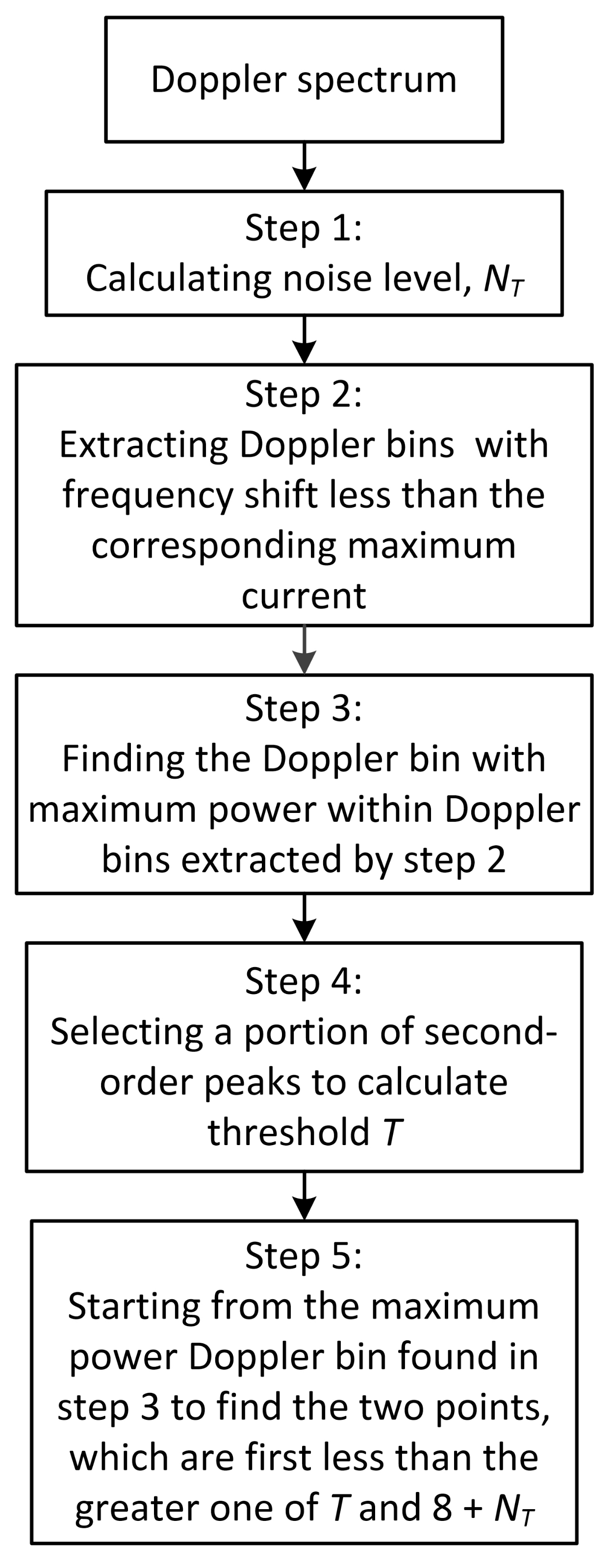
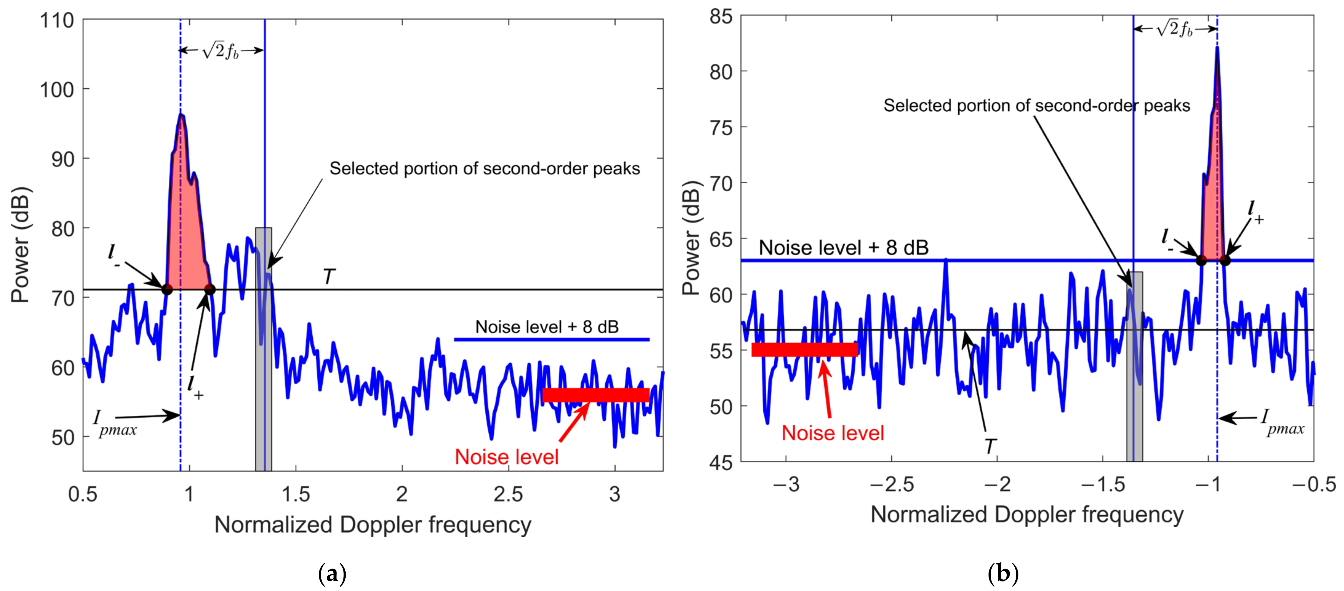
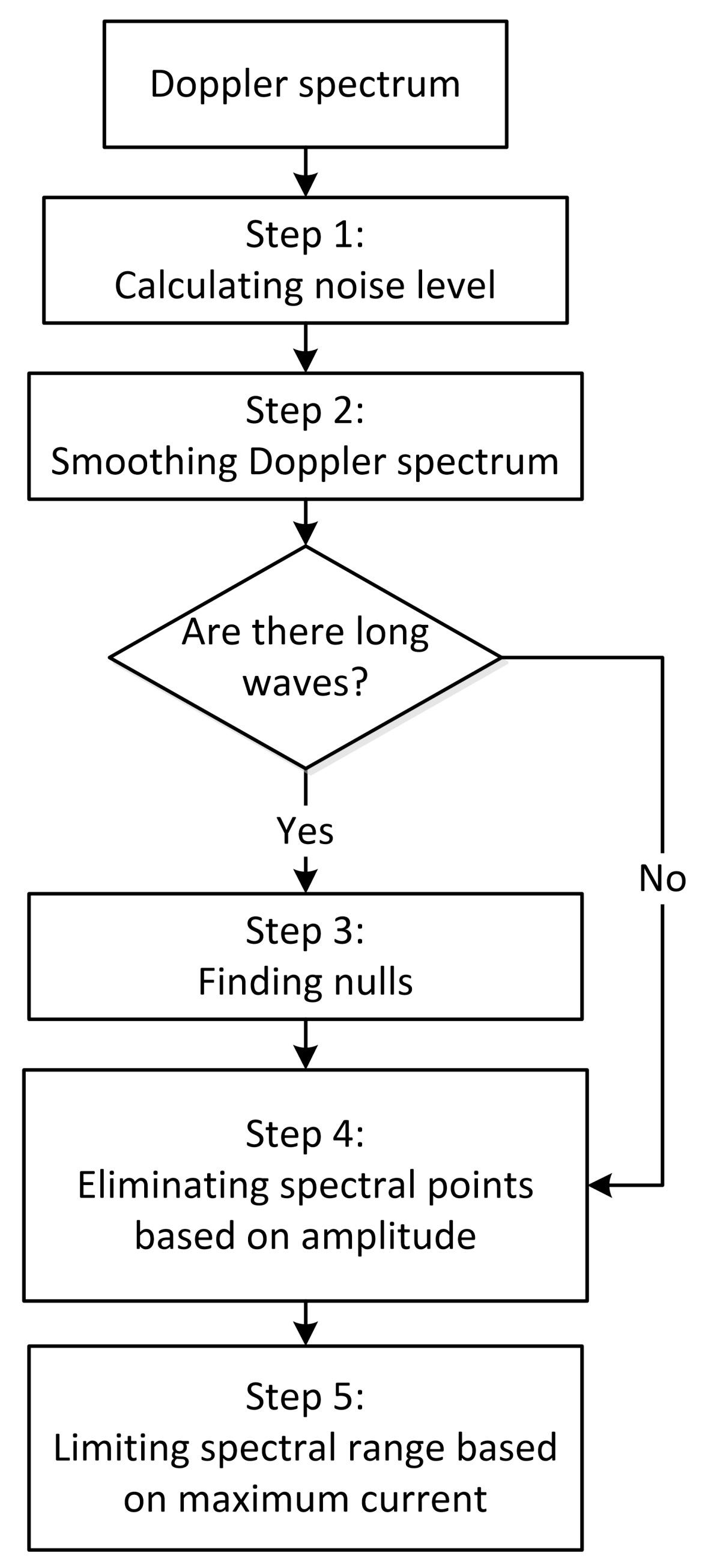
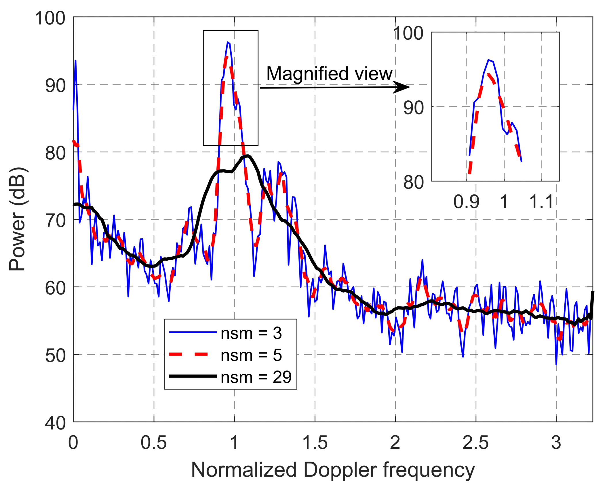
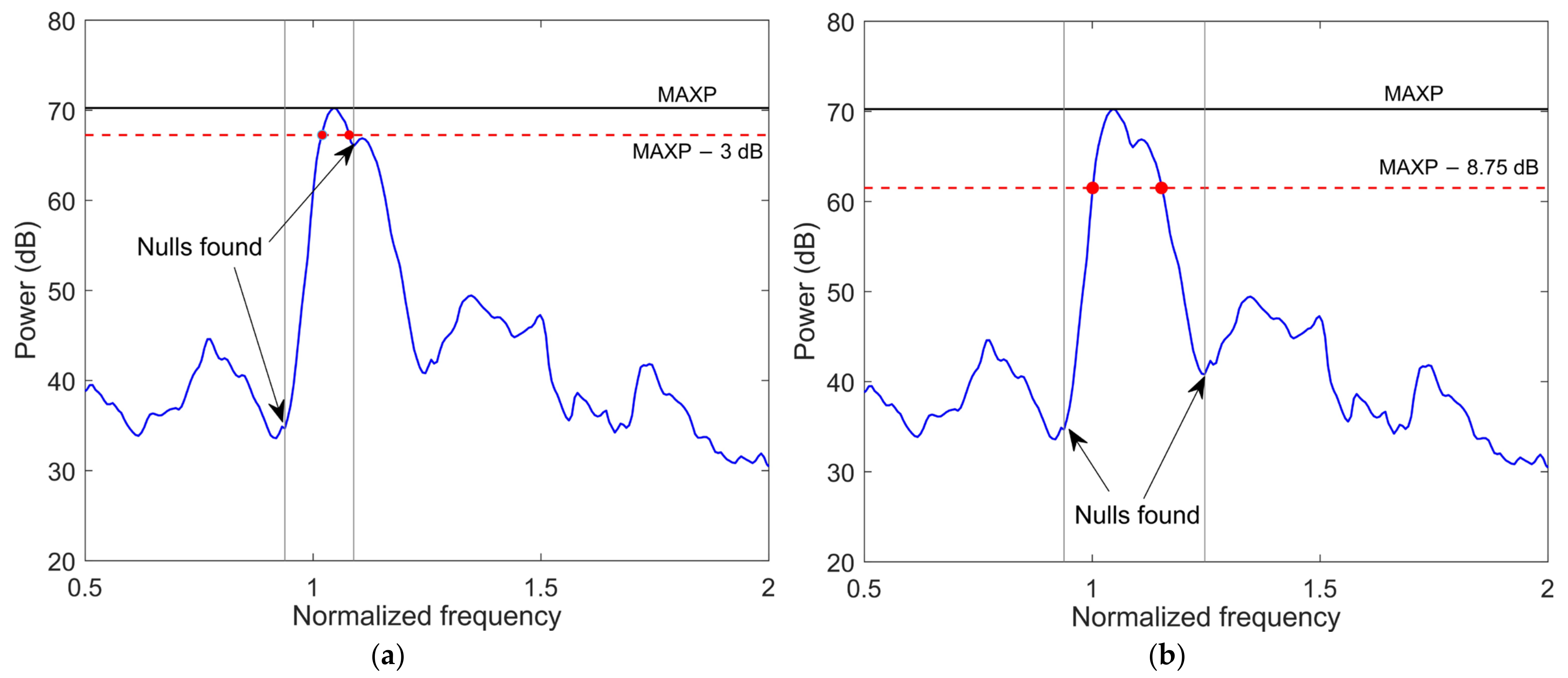
2. The Proposed SSB Method
3. Testing the SSB Method
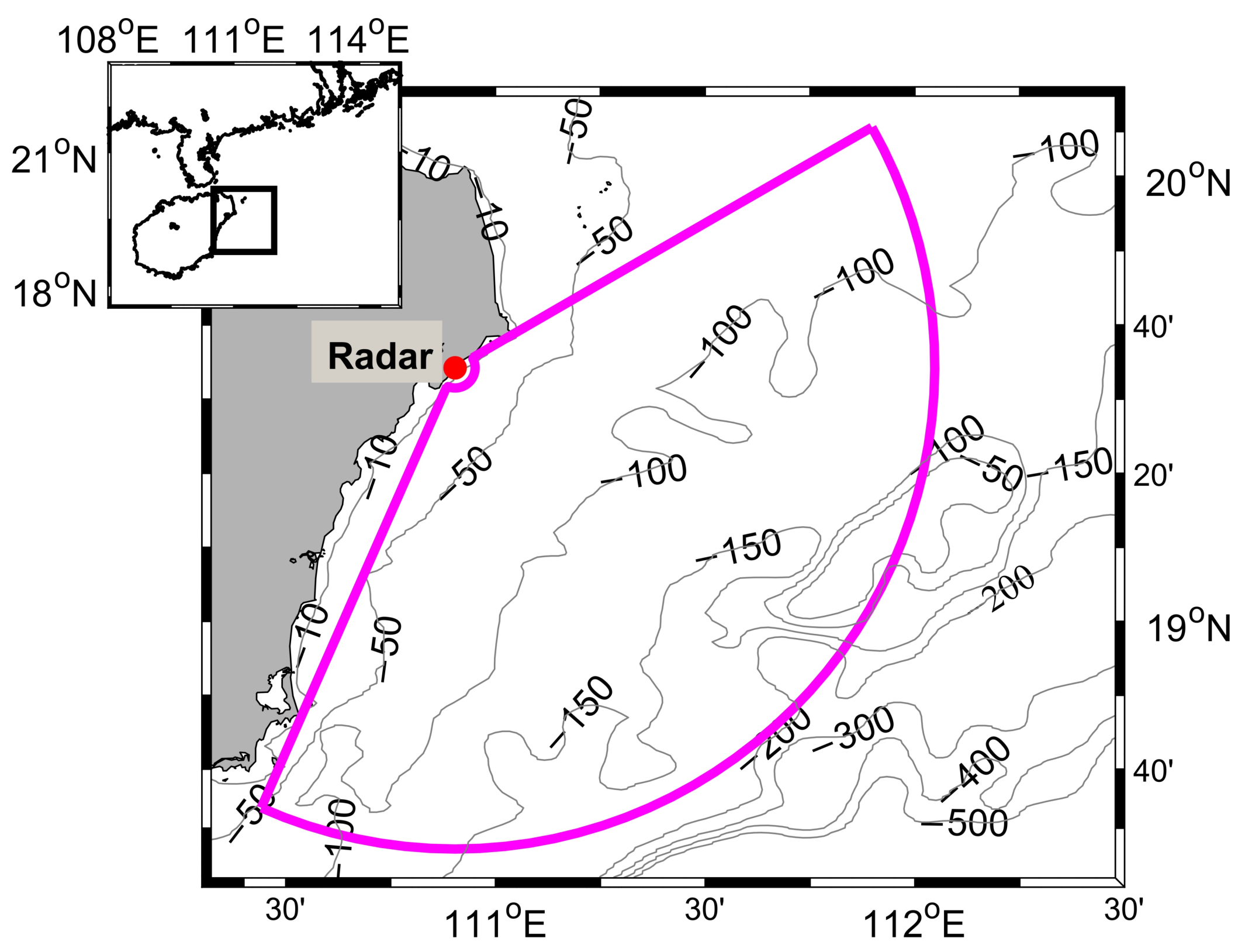
3.1. Test Data Set
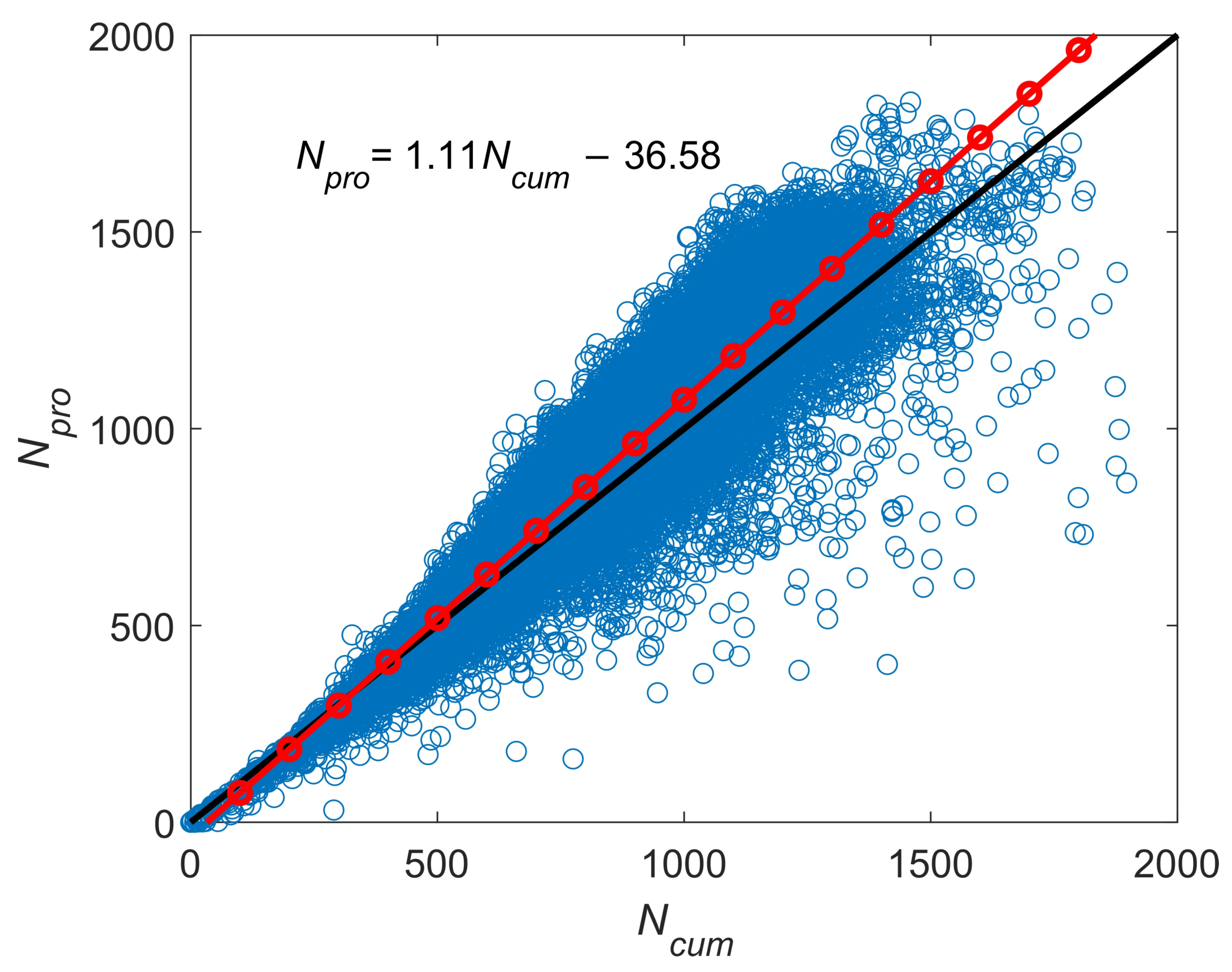
3.2. Results
4. Discussion
5. Conclusions
Author Contributions
Funding
Institutional Review Board Statement
Informed Consent Statement
Data Availability Statement
Conflicts of Interest
Appendix A. The SeaSonde Method


References
- Paduan, J.D.; Washburn, L. High-Frequency Radar Observations of Ocean Surface Currents. Annu. Rev. Mar. Sci. 2013, 5, 115–136. [Google Scholar] [CrossRef] [PubMed]
- Mantovani, C.; Corgnati, L.; Horstmann, J.; Rubio, A.; Reyes, E.; Quentin, C.; Cosoli, S.; Asensio, J.; Mader, J.; Griffa, A. Best Practices on High Frequency Radar Deployment and Operation for Ocean Current Measurement. Front. Mar. Sci. 2020, 7, 210. [Google Scholar] [CrossRef]
- Jena, B.; Arunraj, K.; Suseentharan, V.; Tushar, K.; Karthikeyan, T. Indian Coastal Ocean Radar Network. Curr. Sci. 2019, 116, 372–378. [Google Scholar] [CrossRef]
- Roarty, H.; Cook, T.; Hazard, L.; George, D.; Harlan, J.; Cosoli, S.; Wyatt, L.; Alvarez Fanjul, E.; Terrill, E.; Otero, M.; et al. The Global High Frequency Radar Network. Front. Mar. Sci. 2019, 6, 164. [Google Scholar] [CrossRef]
- Barrick, D. First-Order Theory and Analysis of MF/HF/VHF Scatter from the Sea. IEEE Trans. Antennas Propag. 1972, 20, 2–10. [Google Scholar] [CrossRef]
- Stewart, R.H.; Joy, J.W. HF Radio Measurements of Surface Currents. Deep. Sea Res. Oceanogr. Abstr. 1974, 21, 1039–1049. [Google Scholar] [CrossRef]
- Barrick, D.; Lipa, B.; Crissman, R. Mapping Surface Currents with CODAR. Sea Technol. 1985, 26, 43–48. [Google Scholar]
- Graber, H.C.; Haus, B.K.; Chapman, R.D.; Shay, L.K. HF Radar Comparisons with Moored Estimates of Current Speed and Direction: Expected Differences and Implications. J. Geophys. Res. Ocean. 1997, 102, 18749–18766. [Google Scholar] [CrossRef]
- Gurgel, K.W.; Antonischki, G.; Essen, H.H.; Schlick, T. Wellen Radar (WERA): A New Ground-wave HF Radar for Ocean Remote Sensing. Coast. Eng. 1999, 37, 219–234. [Google Scholar] [CrossRef]
- Barrick, D.E.; Evans, M.W.; Weber, B.L. Ocean Surface Currents Mapped by Radar. Science 1977, 198, 138–144. [Google Scholar] [CrossRef]
- Lipa, B.; Barrick, D. Least-Squares Methods for the Extraction of Surface Currents from CODAR Crossed-Loop Aatenna: Application at ARSLOE. IEEE J. Ocean. Eng. 1983, 8, 226–253. [Google Scholar] [CrossRef]
- Liu, Y.; Weisberg, R.H.; Merz, C.R. Assessment of CODAR SeaSonde and WERA HF Radars in Mapping Surface Currents on the West Florida Shelf. J. Atmos. Ocean. Technol. 2014, 31, 1363–1382. [Google Scholar] [CrossRef]
- Emery, B.; Washburn, L. Uncertainty Estimates for SeaSonde HF Radar Ocean Current Observations. J. Atmos. Ocean. Technol. 2019, 36, 231–247. [Google Scholar] [CrossRef]
- COS. Defining First-Order Region Boundaries. CODAR Ocean Systems Technical Manual. 2002. Available online: http://support.codar.com/Technicians_Information_Page_for_SeaSondes/Docs/Informative/FirstOrder_Settings.pdf (accessed on 22 December 2020).
- COS. SeaSonde Radial Suite Release 7; CODAR Ocean Sensors (COS): Mountain View, CA, USA, 2013. [Google Scholar]
- Kirincich, A. Improved Detection of the First-Order Region for Direction-Finding HF Radars Using Image Processing Techniques. J. Atmos. Ocean. Technol. 2017, 34, 1679–1691. [Google Scholar] [CrossRef]
- Crombie, D.D. Doppler Spectrum of Sea Echo at 13.56 Mc./s. Nature 1955, 175, 681–682. [Google Scholar] [CrossRef]
- Ivonin, D.V.; Shrira, V.I.; Broche, P. On the Singular Nature of the Second-Order Peaks in HF Radar Sea Echo. IEEE J. Ocean. Eng. 2006, 31, 751–767. [Google Scholar] [CrossRef]
- Zhou, H.; Wen, B. Wave Height Estimation Using the Singular Peaks in the Sea Echoes of High Frequency Radar. Acta Oceanol. Sin. 2018, 37, 108–114. [Google Scholar] [CrossRef]
- Tian, Y.; Wen, B.; Tan, J.; Li, Z. Study on Pattern Distortion and DOA Estimation Performance of Crossed-Loop/Monopole Antenna in HF Radar. IEEE Trans. Antennas Propag. 2017, 65, 6095–6106. [Google Scholar] [CrossRef]
- Ivonin, D.V.; Broche, P.; Devenon, J.L.; Shrira, V.I. Validation of HF Radar Probing of the Vertical Shear of Surface Currents by Acoustic Doppler Current Profiler Measurements. J. Geophys. Res. Ocean. 2004, 109. [Google Scholar] [CrossRef]
- Tian, Z.; Tian, Y.; Wen, B.; Wang, S.; Zhao, J.; Huang, W.; Gill, E.W. Wave-Height Mapping From Second-Order Harmonic Peaks of Wide-Beam HF Radar Backscatter Spectra. IEEE Trans. Geosci. Remote. Sens. 2020, 58, 925–937. [Google Scholar] [CrossRef]
- Lai, Y.; Zhou, H.; Zeng, Y.; Wen, B. Accuracy Assessment of Surface Current Velocities Observed by OSMAR-S High-Frequency Radar System. IEEE J. Ocean. Eng. 2018, 43, 1068–1074. [Google Scholar] [CrossRef]
- Lai, Y.; Zhou, H.; Zeng, Y.; Wen, B. Quantifying and Reducing the DOA Estimation Error Resulting from Antenna Pattern Deviation for Direction-Finding HF Radar. Remote Sens. 2017, 9, 1285. [Google Scholar] [CrossRef]
- Lai, Y.; Zhou, H.; Zeng, Y.; Wen, B. Relationship Between DOA Estimation Error and Antenna Pattern Distortion in Direction-Finding High-Frequency Radar. IEEE Geosci. Remote Sens. Lett. 2019, 16, 1235–1239. [Google Scholar] [CrossRef]
- Saha, D.; Deo, M.C.; Bhargava, K. Interpolation of the Gaps in Current Maps Generated by High-Frequency Radar. Int. J. Remote Sens. 2016, 37, 5135–5154. [Google Scholar] [CrossRef]
- Fredj, E.; Roarty, H.; Kohut, J.; Smith, M.; Glenn, S. Gap Filling of the Coastal Ocean Surface Currents from HFR Data: Application to the Mid-Atlantic Bight HFR Network. J. Atmos. Ocean. Technol. 2016, 33, 1097–1111. [Google Scholar] [CrossRef]
- Halle, C. HF Radar Processing Using “Nearest-Neighbor” Statistics; Techreport; University of California, Davis, Bodega Marine Laboratory: Davis, CA, USA, 2008; 26p. [Google Scholar]
- NDBC. Handbook of Automated Data Quality Control Checksand Procedures; NOAA/NDBC: Hancock County, MS, USA, 2009; 78p. [Google Scholar]
- Kirincich, A.R.; De Paolo, T.; Terrill, E. Improving HF Radar Estimates of Surface Currents Using Signal Quality Metrics, with Application to the MVCO High-Resolution Radar System. J. Atmos. Ocean. Technol. 2011, 29, 1377–1390. [Google Scholar] [CrossRef]


Publisher’s Note: MDPI stays neutral with regard to jurisdictional claims in published maps and institutional affiliations. |
© 2020 by the authors. Licensee MDPI, Basel, Switzerland. This article is an open access article distributed under the terms and conditions of the Creative Commons Attribution (CC BY) license (http://creativecommons.org/licenses/by/4.0/).
Share and Cite
Lai, Y.; Wang, Y.; Zhou, H. First-Order Peaks Determination for Direction-Finding High-Frequency Radar. J. Mar. Sci. Eng. 2021, 9, 8. https://doi.org/10.3390/jmse9010008
Lai Y, Wang Y, Zhou H. First-Order Peaks Determination for Direction-Finding High-Frequency Radar. Journal of Marine Science and Engineering. 2021; 9(1):8. https://doi.org/10.3390/jmse9010008
Chicago/Turabian StyleLai, Yeping, Yuhao Wang, and Hao Zhou. 2021. "First-Order Peaks Determination for Direction-Finding High-Frequency Radar" Journal of Marine Science and Engineering 9, no. 1: 8. https://doi.org/10.3390/jmse9010008
APA StyleLai, Y., Wang, Y., & Zhou, H. (2021). First-Order Peaks Determination for Direction-Finding High-Frequency Radar. Journal of Marine Science and Engineering, 9(1), 8. https://doi.org/10.3390/jmse9010008