In-Stream Tidal Energy Resources in Macrotidal Non-Cohesive Sediment Environments: Effect of Morphodynamic Changes at Two Bays in the Upper Gulf of California

Abstract

Because of the need to diversify the renewable energy matrix and because hydrokinetic tidal energy technologies are mature, many in-stream tidal energy resource studies are available globally. Still, there are many questions regarding the effect of seabed changes on tidal energy resources. For coastal regions in particular, where the seabed is generally more mobile than in deep waters, bathymetric evolution could significantly affect tidal energy production. Here, two models are used to analyse the potential effect of natural morphodynamic change on tidal energy resources at two macro-tidal sandy bays, Adaír Bay and San Jorge Bay, in the Upper Gulf of California, Mexico. One of the models is (purely) hydrodynamic, and the other is a morphodynamic model (with hydrodynamic–morphodynamic coupling). The models are validated against tidal current observations obtained with acoustic Doppler current profilers in the region of interest, using three different error statistics, which showed good agreement between models and observations. The results also showed that the most significant bed changes and the largest renewable energy resources are located near the shore. Moreover, there was a good correlation between (a) regions with the most significant depth changes and (b) the areas where the difference in annual energy production with and without depth change was largest. Finally, a two-year simulation with the morphodynamic model permitted to analyse the seabed evolution of a zonal profile off Punta Choya, the headland between the two bays. This profile evolved towards a featureless equilibrium, as expected from the morphological classification for macro-tidal sandy environments under a dominant tidal forcing. However, most importantly, this natural evolution would not be detrimental to tidal energy exploitation at the site.

1. Introduction

The Gulf of California (GC), located in the northwest Mexican coast (See Figure 1), is the only marginal sea in the Eastern Pacific. Many studies (both numerical and observational) have described different oceanographic phenomena in the GC and their dynamics, for example, trapped coastal waves, coastal upwelling, gyre evolution and mixing, or tides and residual tidal currents, to name a few [1,2,3,4].

Some authors have suggested that tides in the GC may be a possible source of renewable energy [4,5]. In the upper GC, located north of the Great Island Region, and in particular close to the head, tides are dominated by the semi-diurnal M₂ principal component, with tidal ranges near the head varying between six and eight meters [3]. Spring-neap cycles are also evident throughout the GC, as observed in tidal gauge data obtained from http://predmar.cicese.mx/ (last accessed on 9 April 2021). Tidal ranges and spring-neap cycle characteristics both affect tidal energy production for tidal lagoon developments. Other studies have also shown that tidal currents are commercially viable energy resources in the Great Island Region and the upper GC [6].

The first analysis assessing the effects of morphology on renewable energy resources used the Infiernillo Channel as a case study [7]. The Infiernillo Channel is a strait between Tiburón Island and Mexico’s mainland; it is around 40 km long and 8 km wide in its widest section. Magar [7] showed that variations of bathymetric conditions had remarkable effects on the monthly tidal power density (TPD) predicted by the models, specifically on the TPD magnitude and the locations of maximum TPD. This dependence of the TPD on the bathymetric input conditions may cause substantial technical impacts on Renewable Energy device deployments.

Coastal headlands are also potential in-stream tidal energy sites because of the local flow accelerations caused by the headland [8]. Therefore, one may envisage assessing the tidal energy resources around headlands within the GC. One such headland is Punta Choya, shown in Figure 1. However, there are no islands in front of it that constrain the flow, as in the Infiernillo Channel, the two headlands delimiting the entrance to Adaír Bay constrict the flow within the Bay. Near Punta Choya, the tidal range is more than six meters, and flow speeds between slack waters could be sufficiently large for in-stream tidal array developments. The energy demand of the region depends on commercial activities and the electricity and illumination needs of nearby towns, and therefore the power transmission lines are well developed [9]. While new renewable energy developments would require an increase in transmission line capacity, having the transmission line infrastructure nearby is advantageous.

Regional models may be used to evaluate either the effect of tidal turbines on the environment or the impact of the environment on the tidal turbines’ efficiency. Chatzirodou et al. [10] and Robins et al. [11] have studied the former in the context of tidal sandbanks and formulated a level of “acceptable change”. This research focuses on the latter by evaluating the effect of morphological change on energy production. Such an effect may be crucial for in-stream tidal plant planning if minor changes in morphology lead to significant changes in possible energy production. This study aims to assess tidal currents and morphological evolution under climatologically mild conditions in the Upper GC region and their effect on the tidal energy resources. We set up two models with high resolution in the area of interest. The models have the same open-boundary forcings at the mouth of the GC and same initial bathymetry, but one of them is only hydrodynamic, and the other is a morphodynamic model. The high-resolution part of the domain covers two macro-tidal bays on the Upper GC’s northeastern side: Adaír Bay and San Jorge Bay (See Figure 1). The models are validated against acoustic Doppler current profiler (ADCP) observations. A climatologically mild year is assumed, so the models are forced only with tides at the open boundary. The flow velocity fields, the mean annual tidal power density (TPD) and the annual energy production (AEP) are determined for one simulation year. The morphodynamic model is run for a second year to assess how the seabed is evolving in the longer term.

The paper is organised as follows. In Section 2, the model equations and the initial and boundary conditions are described, together with the calibration parameters and statistical measures used for the calibration and validation of the models against the ADCP observations. In Section 3, the mean peak flow during spring tides, $U_{STM}$, the annual average of the tidal power density (TPD), and some considerations on the annual energy production (AEP) are presented and discussed. Then, the implications of natural seabed changes for tidal energy resource exploitation in the area are analysed, particularly in the regions with the largest $U_{STM}$, TPD, and AEP values. A two-year simulation is undertaken with the morphodynamic model to assess the seabed evolution over more extended periods. It is worth recalling that the model assumes mild weather conditions and that it is unlikely that this is valid over two years in a row. Still, the study allows us to understand the system’s behaviour when tidal forcings prevail.

2. Materials and Methods

2.1. Description of the Hydrodynamic and Morphodynamic Models

2.1.1. Hydrodynamics Formulation

The numerical simulations of the hydrodynamics for both GC_MD and GC_MD_mor models were carried out with the hydrodynamics modules of Delft3D-FLOW. Delft3D-FLOW solves the incompressible Navier–Stokes equations under the shallow water and the Boussinesq approximations to simulate shallow water flows [12]. In 3D simulations, the default version of Delft3D uses curvilinear coordinates in the horizontal dimensions and $\sigma$ terrain-following coordinates in the vertical dimension [13]. In this work, we implemented the two-dimensional, depth-averaged model with the default coordinate settings.

The depth-averaged system of equations consists of two momentum conservation equations for the velocity components $(U,V)$, a conservation equation for the hydrostatic pressure P, and the continuity (mass conservation) equation for the sea surface height $\zeta$:

$$\frac{\partial U}{\partial t}+U\frac{\partial U}{\partial x}+V\frac{\partial U}{\partial y}-fV=-\frac{1}{{\rho }_0}\frac{\partial P}{\partial x}+F_x+M_x+\nabla ·(D_H\nabla U)+{\tau }_{sx}-{\tau }_{bx},$$

(1)

$$\frac{\partial V}{\partial t}+U\frac{\partial V}{\partial x}+V\frac{\partial V}{\partial y}+fU=-\frac{1}{{\rho }_0}\frac{\partial P}{\partial y}+F_y+M_y+\nabla ·(D_H\nabla V)+{\tau }_{sy}-{\tau }_{by},$$

(2)

$$P=g{\rho }_0(\zeta +d),\mathrm{and}$$

(3)

$$\frac{\partial \zeta }{\partial t}+\frac{\partial \left[\right(\zeta +d\left)U\right]}{\partial x}+\frac{\partial \left[\right(\zeta +d\left)V\right]}{\partial y}=0,$$

(4)

where $\zeta$ is measured from the reference level corresponding to mean sea level (MSL) and d is the water depth from MSL, defined as positive downwards. The terms $(F_x,F_y)$ are the components of a vector force representing the unbalance of the horizontal Reynolds stresses; the Reynolds stresses are modelled using the eddy viscosity concept introduced by [14]. The forces $(F_x,F_y)$ are necessary because, although the model is capable of resolving the turbulent scales, usually the hydrodynamic grids are too coarse to resolve the fluctuations. Therefore the momentum equations are Reynolds-averaged, introducing so-called Reynolds stresses. The Reynolds stresses are related to the Reynolds-averaged flow quantities through a turbulence closure formulation. $(M_x,M_y)$ are the external forcing and source/sink terms due, for instance, to discharge or withdrawal of water, water-structure interactions, or wave stresses; $D_H$ is the depth-averaged horizontal turbulent eddy viscosity, and ${\tau }_s-{\tau }_b$ represents the difference between the surface and the bottom shear stresses, respectively [15].

2.1.2. Sediment Transport and Morphodynamics Formulations

The sediment transport and morphodynamics are solved with an advection-diffusion equation and with Exner’s equation, respectively. For the GC_MD_mor model setup, we assumed that the seabed was mainly composed of non-cohesive sediments with a median sediment diameter D₅₀ of 200 µm, corresponding to a sandy seafloor; a specific density of 2650 kg m⁻³; a dry bed density of 1600 kg m⁻³; and an initial sediment layer thickness of 5 m. Note that in the northeastern side of the Upper GC, the sediment on the seafloor varies from medium to fine sand, as one can see from Figure 2 (modified from [16]). Figure 2 shows that in the high-resolution sub-domain (see Figure 3) D₅₀ is larger than 7.8 µm, and generally between 62.5 µm and 0.25 mm close to the coast, which corresponds to the range for non-cohesive sediments. This sediment composition agrees with the qualitative sediment sample observations we performed during the fieldwork campaigns of 2017 and 2018. Note that Carriquiry et al. [16] had very few sediment sampling stations in Adaír Bay and San Jorge Bay. However, since we have no riverine sources of sediment and no mangrove or saltmarsh fields with high organic content in Adaír Bay and San Jorge Bay, it is justifiable to assume that the sediments here are mostly non-cohesive. Thus, it is reasonable to take a uniform median grain diameter of the order of $0.2$ mm throughout the study region as a first modelling approximation.

Van Rijn’s model for sediment bedload and suspended load transport is used in the computations [17]. In this approach, the suspended sediment concentration C of the single sediment fraction [in kg m⁻³], satisfies in the depth-average formulation a two-dimensional advection-diffusion equation of the form:

$$\begin{array}{c}\hfill \frac{\partial \left[\left(\zeta +d\right)C\right]}{\partial t}+\frac{\partial \left[\left(\zeta +d\right)UC\right]}{\partial x}+\frac{\partial \left[\left(\zeta +d\right)VC\right]}{\partial y}=\\ \hfill \left(\zeta +d\right)\left[\frac{\partial }{\partial x}\left(D_H\frac{\partial C}{\partial x}\right)+\frac{\partial }{\partial y}\left(D_H\frac{\partial C}{\partial y}\right)\right]+\left(\zeta +d\right)S,\end{array}$$

(5)

where $(U,V)$ are the depth-averaged flow velocity components (m s⁻¹), $D_H$ the sediment diffusivity (m² s⁻¹), and S the sediment source/sink terms (kg m⁻³ s⁻¹). The bottom boundary condition for non-cohesive sediments is a balance between the erosion (E) and deposition (D) flux terms, which in turn depend on the settling processes at a bottom reference bed level $z=z_b$:

$$E-D=w_{s}C,$$

(6)

with $w_s$ the (terminal) settling velocity (m/s). As there are neither estuaries nor other sources of sediment discharge in the area of interest, the source/sink terms in Equation (6) are directly linked to $E-D$, as defined in Equation (6). The model also includes a bedload transport formulation that is considered in the bathymetric evolution, the reader is referred to the Delft3D manual for further information [15]. As mentioned above, the same timestep is used for the momentum and the advection-diffusion equations. Note that model outputs, both at the observation points and in map format, are stored at 30-minute intervals only due to data storage constraints.

2.2. Boundary Conditions

2.2.1. Tidal Forcing Assumptions

Gross and Magar [18] ran a simulation that included the potential tidal forcing over the whole domain and the tidal forcing at the mouth of the GC. They concluded that the potential tidal forcing effect was negligible compared to that caused by the co-oscillation with the Pacific Ocean at the mouth. Therefore, here both the GC_MD and GC_MD_mor models were forced at the mouth of the GC with 13 principal tidal harmonics (M2, S2, N2, K2, K1, O1, P1, Q1, MF, MM, M4, MS4, MN4) from the TPXO8.1 model, a Global Inverse Tidal Model [19,20]. The tides were the only forcing implemented in the model because we assumed climatologically mild conditions, and thus the tides dominate over other forcing mechanisms. This assumption is justified because the renewable energy resources generated by tidal currents in this region are significantly larger than those generated by wind-driven currents, even during a climatologically average year (see [6] for more details).

2.2.2. Bathymetry

The bathymetry chosen for the simulations was the General Bathymetric Chart of the Oceans (GEBCO2014). GEBCO2014 has a spatial resolution of approximately 900 m (see Figure 1). Because the GEBCO data was unreliable in the coastal lagoons, some regions were masked. Since this work focuses on the offshore regions around the coastal shoals of Adaír Bay and the areas in the two bays with water depths of 10 m or more, this masking does not affect the results presented here. Depth outliers in other parts of the domain were also removed. It is worth highlighting that although the Navy and other institutions provided some gridded bathymetry data obtained with in-situ surveys, their coverage was very small compared to the region of interest, and the resolution was also 900 m.

2.3. Spatio-Temporal Discretisation

2.3.1. Sub-Domain Selection

The morphodynamic model GC_MD_mor is equal to the hydrodynamic model GC_MD extended with sediment transport and morphological updating of the bathymetry. In both models, the computational domain is split into three sub-domains: A coarse domain d01 with a spatial resolution of 6480 m covering the western approach (where it connects to the Pacific Ocean) and the deep parts of the GC; an intermediate domain d02 with a spatial resolution of 2160 m in the coastal regions and the north part of the Gulf; and an inner domain d03 with a resolution of 240 m covering Adaír Bay and San Jorge Bay, located in the Northeastern part of the Gulf. The area covered by each of the three sub-domains is shown in Figure 3, with particular emphasis on the sub-domain with the highest resolution, namely d03, with grid cell size $\Delta x=240$ m. The grids are regular with square cells and are orientated roughly along the longitudinal axis of the GC. The communication between sub-domains occurs along the d01-d02 and the d02-d03 boundaries. All the sub-domains need to have the same parameter settings and timestep intervals, which increases computational costs. However, these costs can be compensated by carrying out the computations separately (using P-threading) at each sub-domain [15]. In fact, the domain-decomposition approach is more flexible, accurate, and generally faster than other nested or unstructured grid techniques.

2.3.2. Timestep Selection

The timestep used for all sub-domain computations is determined using the Courant–Friedrichs–Lewy (CFL) parameter, establishing a theoretical stability condition for sub-domain d03. In general terms, the CFL parameter is defined as:

$$CFL=\frac{u\Delta t}{\Delta x},$$

(7)

where u is a characteristic speed, $\Delta t$ the model timestep, and $\Delta x$ = 240 m the grid size of the highest-resolution sub-domain, d03. For Delft3D-FLOW, in general, $CFL<10$ is sufficient to achieve model stability. For this condition to hold in sub-domain d03, it was sufficient to take $\Delta t$ = 60 s. The same timestep is used in both the GC_MD and GC_MD_mor models. Some authors use a morphodynamic acceleration factor, $MORFAC$ [15],

$$\Delta t_{\mathrm{mor}}=MORFAC\times \Delta t,$$

where $\Delta t_{\mathrm{mor}}$ is the morphological timestep, and $\Delta t$ the hydrodynamical timestep already discussed above. $MORFAC$ generally is 3 to 10, or even larger, but the morphodynamic model still needs to be calibrated and tested with $MORFAC=1$. Therefore, here we set $\Delta t_{\mathrm{mor}}$ equal to the $\Delta t$ satisfying the $CFL$ condition in the sub-domain d03.

2.4. Calibration and Validation of the Models

The models were calibrated and validated using the tidal signal extracted from the model and from in-situ measurements. Because the hydrodynamic assumptions in both models are identical, we used GC_MD for the calibration and validation. The in-situ water levels and flow velocities were obtained from bottom-mounted acoustic Doppler current profilers (ADCPs) that we installed between 2017 and 2019 at three different locations (see in Figure 1). SJI1 and SJI2 were installed near San Jorge Island, and AB was installed west of Punta Choya in Adaír Bay. The average water depth at SJI1 was 16 m, and the average tidal range was 6.5 m. The average water depth at SJI2 was 22 m, and the average tidal range was 6.3 m. The average water depth at AB was 17 m, and the average tidal range was 7.3 m. The ADCPs were used either for calibration or validation according to their location and period of operation (the dates are in dd/mm/yyyy format):

• SJI1₁₇: Operational from 05/06/2017 to 26/11/2017. Used for calibration.
• SJI1₁₈: Operational from 22/06/2018 to 06/11/2018. Used for validation.
• SJI2: Operational from 21/06/2018 to 21/11/2018. Used for validation.
• AB: Operational from 14/12/2018 to 14/05/2019. Used for validation.

The ADCPs sampled at a frequency of one Hertz, but only 30-min or 60-min averages were stored in memory. Measurements were taken at one-meter intervals and 2.10 m upwards from the seafloor for SJI1₁₇, and 1.89 m upwards for the other monitoring campaigns. The measurement cells closest to the sea surface were removed due to the signal’s contamination by sound reflections from the water-air interface. The remaining cells’ data was depth-averaged, and we computed the tidal signal using the t_tide program [21]. t_tide was also used to determine the tidal signal from the depth-averaged velocities predicted with the model. An example of the reconstructed tidal signals is shown in Figure 4, for the GC_MD_mor model, and the data obtained with the ADCP in Adaír Bay. It is important to note that the tidal speed peak signal’s timings obtained with the models and those in the ADCP observations are almost the same, as one can see from Figure 4 and Figure 5. This is expected because of the predictability of tides. Therefore, only the velocity magnitudes are used for calibration and validation.

The model skill was assessed by determining the agreement between model $X=U_{mod}$ and ADCP data $Y=U_{obs}$, for the reconstructed tidal signal. This agreement was analysed by comparing the Pearson correlation coefficient, ${\displaystyle {\rho }_{X,Y}}$ [-] (non-dimensional), defined as [22]:

$${\rho }_{X,Y}=Cor{r}_U=\frac{cov(X,Y)}{{\sigma }_X{\sigma }_Y},$$

(8)

where cov is the covariance between the two time series, and ${\sigma }_X$ and ${\sigma }_Y$ the standard deviations of X and Y, respectively; the root mean square error, $RMS{E}_U$, [m s⁻¹]:

$$RMS{E}_U=\sqrt{\frac{1}{N}\sum _{i=1}^N{\left(U_{mod,i}-U_{obs,i}\right)}^2},$$

(9)

and at times the absolute relative error, $R{E}_U$ [%],

$$R{E}_U=∥\frac{{\overline{U}}_{obs}-{\overline{U}}_{mod}}{{\overline{U}}_{obs}}∥\times 100.$$

(10)

The time interval used for the model-measurement intercomparisons was 30 min at the SJI1₁₇, SJI1₁₈ and SJI2 moorings, and 60 min at the AB mooring.

2.4.1. Calibration Results

We compared the tidal signal predicted by the model against the tidal signal observed at SJI1₁₇ over part of the sampling period to calibrate the model parameters. The parameters we varied were the reflection parameter (dimensionless), the horizontal viscosity (m² s⁻¹), and the friction coefficient $C_f$ (m^1/2 s⁻¹). The reflection coefficient was introduced by Stelling [12] in the boundary conditions to make the boundaries less reflective for disturbances with the eigenfrequency of the model area; in ocean and sea models, it is recommended to set it to zero ([15], p. 203). The horizontal viscosity, on the other hand, is a parameter usually tuned according to the grid cell size, as it may affect model stability ([15], p. 371). For models with cell sizes between 20 and 40 m, a horizontal viscosity of 0.5 m² s⁻¹ works well. For grids with cell sizes in the order of 100 m, the default value of 1 m² s⁻¹ is reasonable. Preliminary results showed that the model predictions were not very sensitive to slight variations of the reflection parameter or the horizontal viscosity [23], so we set them to the default values. Thus, we only tested in detail the model sensitivity to variations of the friction coefficient $C_f$, based here on the Chézy formulation.

Table 1. Model calibration for the period of 04/06/2017–04/07/2017 (without the spin-up time).

${\mathit{C}}_{\mathit{f}}$	${\mathit{Corr}}_{\mathit{U}}$	${\mathit{RMSE}}_{\mathit{U}}$
100	0.6992	0.1122
80	0.7232	0.1077
65	0.7910	0.1034
60	0.7962	0.1018
55	0.7503	0.1001
45	0.7533	0.0972

shows $Cor{r}_U$ and $RMS{E}_U$ for seven values of $C_f$ (m^1/2 s⁻¹), for simulations that were run from StartTime = 01/06/2017 to EndTime = 04/06/2017. The first three days were the model’s spin-up time and were discarded in the computation of the errors. The final $C_f$ was taken as 45 m^1/2s ⁻¹, when $RMS{E}_U$ is smallest. Note that we expected that we would need to reduce the default value of $C_f$ to values around 45 m^1/2 s⁻¹, based on results by Baston et al. [24]. It was also for this value of $C_f$ when the plots of modelled and observed tidal signals, such as the one shown in Figure 4 for AB, looked best.

2.4.2. Validation Results

We used the ADCP moorings SJI1, SJI2 and AB, introduced in the previous section, to validate the results obtained with the models.

Table 2. Validation of GC_MD (first 4 rows) and GC_MD_mor (last row) at the ADCP locations.

Model	Mooring	Period (StartTime-EndTime)	$\overline{\mathit{U}}$ mod/adcp	${\mathit{Corr}}_{\mathit{U}}$	${\mathit{RE}}_{\mathit{U}}$	${\mathit{RMSE}}_{\mathit{U}}$
GC_MD	SJI117	05/06/2017–26/11/2017	0.23/0.22	0.8766	20%	0.0685
GC_MD	SJI118	22/06/2018–06/11/2018	0.23/0.19	0.8880	21%	0.0692
GC_MD	SJI2	21/06/2018–21/11/2018	0.22/0.23	0.7072	1.6%	0.1150
GC_MD	AB	14/12/2018–14/05/2019	0.16/0.15	0.8681	6.1%	0.0567
GC_MDmor	SJI117	05/06/2017–26/11/2017	0.29/0.22	0.8815	9%	0.2938

summarises the results of these validations for the yearly mean speed, $\overline{U}$, obtained from the depth-averaged model predSictions (mod) and ADCP observations (adcp) of the flow speed.

Overall, the correlation coefficient, the RE and the RMSE values obtained in the modelled-observed speed comparisons were acceptable, even though one may consider that a relative error of around 20% is at the limit of the acceptability threshold. SJI2 was the location and monitoring period with the smallest relative error, but a relatively large RMSE of 0.115 m/s. This large RMSE for the flow speeds causes significant errors for the TPD and the AEP validations at this location. We obtain the best agreement between the GC_MD model and the ADCP reconstructed tidal speed time series at the AB mooring, shown in Figure 4. However, in some tidal cycles, GC_MD seems to overestimate the flow speed.

To validate the morphodynamic model GC_MD_mor, we used the depth-averaged reconstructed tidal ADCP measurements taken at the SJI1₁₇ mooring, and the corresponding depth-averaged, reconstructed tidal signal predicted by GC_MD_mor. We found a good correlation of 0.88 (see Table 2) and an excellent relative error of 9% between model and measured data, but in Figure 5 we see that the GC_MD_mor model overestimates the flow speeds at the ADCP moorings. Table 2 shows the value of the $RMS{E}_U$, which is quite high, considering the mean values of the velocity field at this location, also shown in Table 2.

3. Results and Discussion

We ran a one-year simulation of the GC_MD and GC_MD_mor with the calibrated parameters, to map and analyse the yearly averaged spring tidal speed maxima, $U_{STM}$, the yearly averaged Tidal Power Density (TPD), and the Annual Energy Production (AEP). The instantaneous TPD, $TP{D}_i$, is defined as:

$$TP{D}_i=\frac{1}{2}\rho U_i^3,$$

(11)

with $U_i$ being the instantaneous speed. Its mean is defined simply as

$$TPD=\frac{1}{N}\sum _{i=1}^{N}TP{D}_i,$$

(12)

and the AEP is defined as:

$$AEP=\sum _{i=1}^{N}TP{D}_i.$$

(13)

Here N is the total number of hourly data in the simulated year, or the number of times when $TP{D}_i$ is above the threshold value of 50 W m⁻², depending on the variable used. This technical TPD threshold corresponds to a low-speed threshold of 0.46 m s⁻¹, typical of most tidal energy devices, as discussed in [6].

The mean spring tidal speed maxima, $U_{STM}$, is computed by identifying the maximum flow speed in spring tides, which for the year of simulation gives 26 maxima, and then computing the mean of those values.

3.1. Analysis of $U_{STM}$

Figure 6 shows the yearly mean of the spring tidal maxima flows, $U_{STM}$, for the GC_MD (Subplot 1) and the GC_MD_mor models (Subplot 2). The largest $U_{STM}$ values in San Jorge Bay were also on or near regions with bottom sand ridges, but the effect of the bottom bathymetry is more noticeable in Adaír Bay. The largest values of $U_{STM}$ were observed as well in the nearshore of Adaír Bay, where we have a series of shoals, with the site just North of Punta Choya (see Figure 1) being the most important region for tidal energy resources.

It was expected that Punta Choya would play an essential role for tidal energy resources because it is a headland, and other researchers have observed that coastal flows tend to accelerate around headlands [8]. It is worth mentioning that these possible tidal energy exploitation sites had not been identified with low-resolution models [6], which highlights the limitations of those models for nearshore tidal energy characterisation.

Figure 6 also shows the effect of coastal morphodynamics on the spring tidal maxima flows, for example, that the areas where the yearly averaged $U_{STM}$ is 1 m s⁻¹ or above expand when the bottom is allowed to evolve under tidal action. This effect will be explored in more detail using the yearly tidal power density.

3.2. Analysis of TPD

Figure 7 shows the yearly mean TPD obtained for the GC_MD model (Subplot 1) and the morphodynamic model GC_MD_mor model (Subplot 2) over the simulation year. We found areas in the nearshore region of Adaír Bay, where the maximum TPD values are above 200 W/m², but in general below 400 W/m². We observe TPD values that are significantly lower than those reported for the seven US sites analysed in the Tidal In-Stream Energy Conservation (TISEC) program [25]. The TISEC site with the lowest power density was Head Harbour Passage (New Brunswick), with a TPD of 940 W/m². In contrast, the Minas Passage in Nova Scotia has a TPD of 4.5 kW/m², i.e., more than 20 times larger than the largest TPD observed in our study site. For sites with lower TPD, the return on investment will take longer. Small scale also increases the costs by a factor of three [25], and this applies to pilot sites. Despite these drawbacks, this site could still be a useful test site for some devices.

As mentioned in the previous section, the best tidal current energy resources are located off the headland separating Adaír Bay and San Jorge Bay, but other tidal current energy hot spots can also be observed along the eastern coast of Adaír Bay. These regions are, consistently, in the same locations of the domain in the GC_MD and the GC_MD_mor models. However, in GC_MD_mor, the regions with high TPD are spread over larger areas. We observe, in general, an increase in yearly averaged TPD throughout Adaír Bay in the GC_MD_mor model, in comparison with the GC_MD model. At locations marked (a) and (b) in Figure 7, for example,

$$\%\left(TPD\right)=\frac{TP{D}_{\mathrm{mor}}-TPD}{TPD}$$

is of 34.40% at (a) and 69.25% in (b), respectively (the absolute TPD values at (a), (b), (c) and (d) are reported in

Table 3. Water depth (m), yearly TPD (W m⁻²), and AEP (kWh m⁻²) in the GC_MD and GC_MD_mor models, at the selected sample locations.

Loc	${\mathit{d}}_{\mathit{i}}$	${\mathit{d}}_{\mathit{f}}$	${\displaystyle \frac{{\mathit{d}}_{\mathit{f}}-{\mathit{d}}_{\mathit{i}}}{{\mathit{d}}_{\mathit{i}}}}$	TPD	TPDmor	%(TPD)	AEP	AEPmor
a	5.7	7	22.8	128.13	172.32	34.48	1122.6	1509.7
b	11	11.03	0.27	63.71	107.83	69.25	558.16	944.72
c	2.7	2.9	7.41	95.26	79.16	−16.9	834.61	693.53
d	30.32	30.31	−0.033	25.3	48.39	91.26	221.66	423.96

). However, initially the TPD at (a) is much larger than at (b), so even if percentually the yearly TPD does not increase as much in (a) as in (b), the tidal current energy resource is still better at (a). At location (c) in the nearshore of San Jorge Bay, in contrast, the tidal current energy resource decreases in GC_MD_mor in comparison to GC_MD, by 16.9%. Finally, at location (d), %(TPD) = 91.26%, but initially the tidal current energy resources are the lowest here, and therefore it remains low in GC_MD_mor. Please note that %(AEP) = %(TPD).

3.3. Analysis of AEP

Figure 8 shows the AEP maps, with contours of 500 kWh m⁻² delimiting high-energy regions in Adaír bay; these contours can be seen in the results for both the GC_MD (subplot 1a) and the GC_MD_mor models (subplot 2a). When using the GC_MD_mor model (subplot 2a), i.e., when the seabed evolves in time, these high-energy regions cover a much larger area. In particular, the region with maxima AEP located at the southeastern boundary of Adaír Bay extends further to the west in the model GC_MD_mor, in comparison to GC_MD. In the plots 1b and 2b of Figure 8, we also observe this spreading of what we may call good sites for tidal energy exploitation, as measured by the spread of the 200 kWh m⁻² contour, extending in San Jorge Bay in GC_MD_mor, and an increase from 200 to 400 kWh m⁻² in the locations of large AEP. However, in San Jorge Bay these regions are significantly smaller than in Adaír Bay, for both the GC_MD (plot 1a vs plot 1b in Figure 8) and the GC_MD_mor models (plot 2a vs. plot 2b in Figure 8). We can identify the sites with the best renewable energy resources from the AEP maps. Most importantly, however, is the fact that the plots in Figure 8 show the impact of natural seabed evolution on areas with exploitable renewable energy resources. Indeed, within a year the size of such regions has more than doubled in Adaír Bay, a reassuring result for any would-be tidal energy developer interested in implementing a tidal energy demonstration plant in the region.

3.4. Technical Constraints

Some devices, such as Flumill [26] for deployments in waters as shallow as 10 m and up to 50 m deep, or Minesto [27] for deep water deployments, can operate at the low tidal stream speeds of around 1.0 m s⁻¹ that are found in some locations in the Adaír and San Jorge Bays (as shown in Figure 6). Another technical constraint to consider is the cut-in speed. Most commercially viable technologies require cut-in tidal speeds of around 0.5 m s⁻¹ before they start generating any power from the flow; this cut-in speed corresponds to $TPD=$ 50 W m⁻². In Figure 9 and Figure 10, we only consider TPD values of 50 W m⁻² or above, defined as $TPD=TP{D}_{>50}$, and use this for the corresponding computations of $AEP=AE{P}_{>50}$ in Figure 10. The mesh resolution of 240 m, combined with the 30-arcsecond resolution (equivalent to around 900 m) for the bathymetry, gives a better representation of the tidal energy resources in shallow regions in comparison to the global model used by [6]. However, we observe that the global model (Figure 5 of [6]) and the GC_MD model (left subplot, or subplot 1, in Figure 9 in this paper) both show that the northern side of San Jorge Bay, and the nearshore areas in Adaír Bay, do not provide commercially viable conditions for in-stream tidal energy exploitation. Despite this, we can also see some areas with $TP{D}_{>50}$ over 200 W m⁻² in Adaír Bay, such as the nearshore area marked as (a) in Figure 9 and Figure 10, or the area at the southern edge of Adaír Bay marked as (b). Unfortunately, at the observation point $AB$ inside Adaír Bay, we obtained low TPD values and a correspondingly low AEP, but this does not affect the use of $AB$ for model validation purposes. The area marked (c) in San Jorge Bay is the only area in this Bay with $TP{D}_{>50}$ above 200 W m⁻². As can be seen on the left subplot of Figure 10, the area (a) has the largest $AE{P}_{>50}$ of the four marked regions. In fact, at (a) the AEP obtained after one year with the model GC_MD is actually 1122.6 kWh m⁻², as shown in Table 3. The only place where such high values of AEP are observed is in the nearshore region of Adaír Bay.

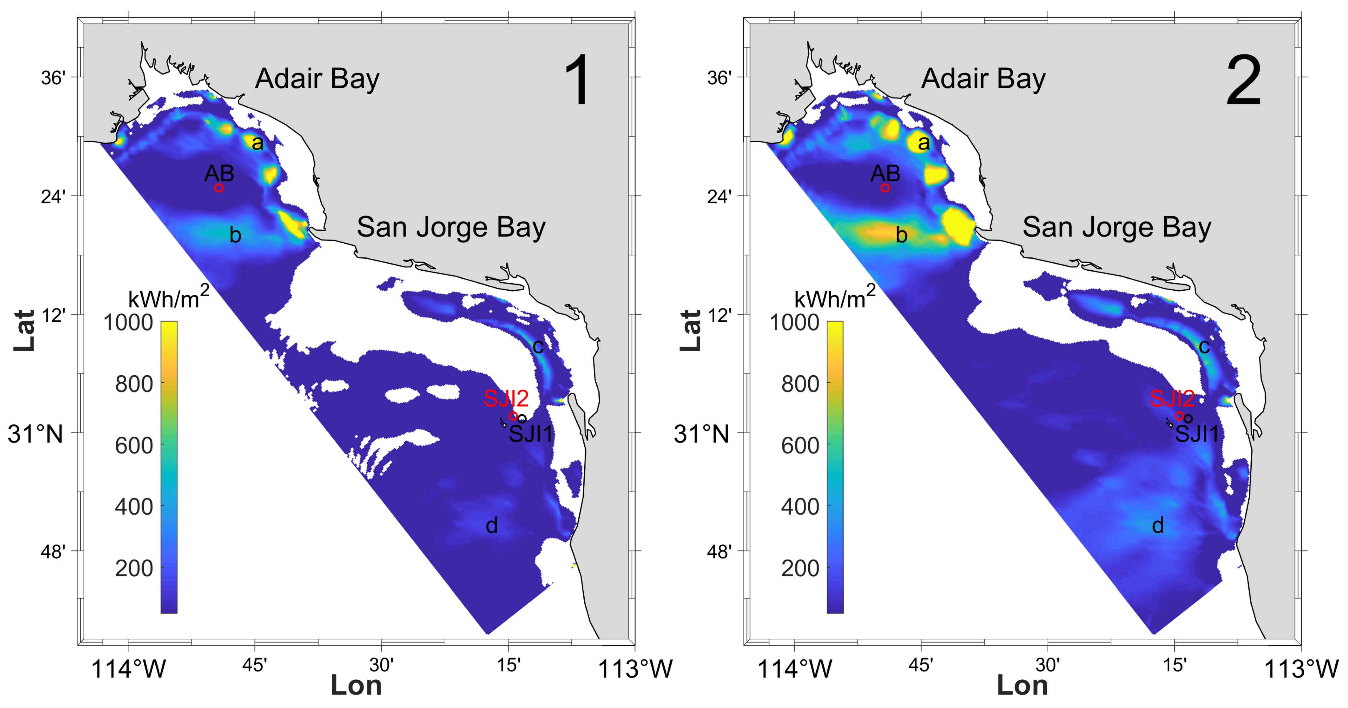
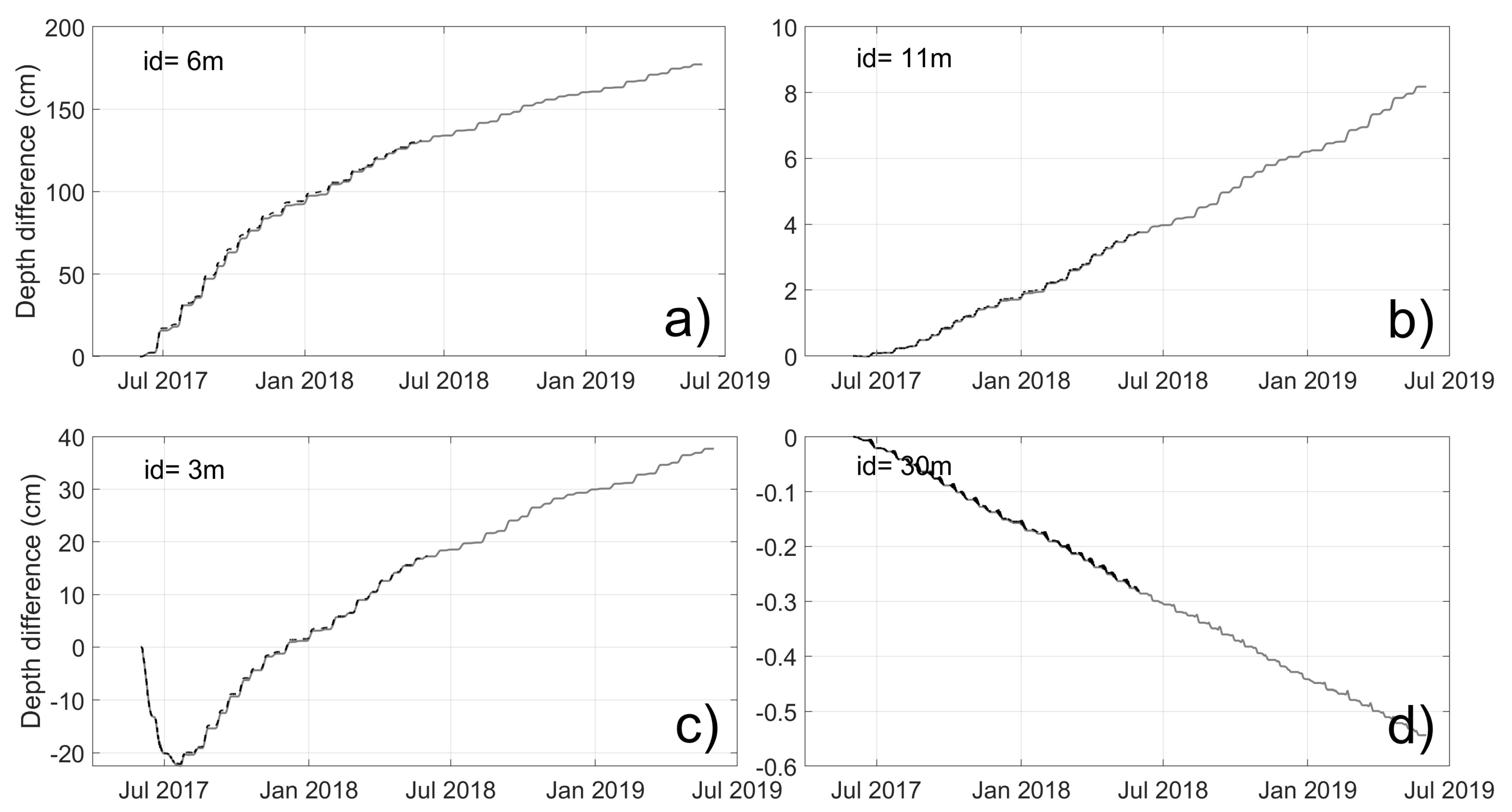
3.5. Effects of Morphological Evolution on Tidal Energy Resources

Figure 9 and Figure 10 show the predicted $TP{D}_{>50}$ and $AE{P}_{>50}$ for the GC_MD (on the left) and the GC_MD_mor (on the right) models. Firstly, we observe that the best locations for in-stream tidal energy exploitation do not shift in space after one year when we have seabed changes (model GC_MD_mor results on the right) in comparison to when we have a fixed bathymetry (model GC_MD results on the left). In Adaír Bay, the area covered by these locations increases in the GC_MD_mor model, which is reassuring as the seabed in this region is naturally mobile, and therefore the GC_MD_mor predictions are expected to be closer to reality. In contrast, in San Jorge Bay, although we see an increase in in-stream tidal energy resources predicted by GC_MD_mor at the locations where the resources were good in GC_MD, the area they cover does not increase in comparison to the area they cover in the GC_MD simulation. While the resources remain marginally exploitable in both simulations, these analyses indicate that Adaír Bay is a better location than San Jorge Bay for a demonstration in-stream tidal energy site, and its suitability improves when the tides force the seabed to evolve, at least in the first year.

We consider now the percentage of time, $\%T$, when the TPD is equal or above the cut-in TPD of 50 W m⁻², and evaluate the impact of morphodynamic evolution. Subplots 1a and 1b in Figure 11 show $\%T$ when TPD is above 50 W m⁻², for the GC_MD model, and subplots 2a and 2b in Figure 11 show $\%T$ when TPD is above 50 W m⁻², for the GC_MD_mor model. The maps in subplots 1a and 2a show Adaír Bay, where we can identify regions where TPD is above 50 W m⁻² for more than 40% of the time, for both for GC_MD and GC_MD_mor. There are also vast regions in Adaír Bay where $\%T$ is close to 60%. Figure 11 shows results that are consistent with those in Figure 9 and Figure 10, obtaining good agreement between areas with the largest $TP{D}_{>50}$ and $AE{P}_{>50}$ and areas with the largest $\%T$. We also note that the region along and near the same longitude as that of location (b) (see Figure 9), is the region with the largest morphological changes near the coast, in particular close to the eastern shore of the bay, but this impact is positive from an in-stream renewable resource perspective. On the other hand, in San Jorge Bay we found that the percentage of time when TPD is above the cut-in value is generally below 40% (Subplots 1b and 2b in Figure 11), and in the GC_MD model (no morphodynamics), the regions satisfying this constraint are quite small (Figure 11, 1b). These results show that the optimal location for tidal energy resource exploitation is near the southeastern corner of Adaír Bay, west of the peninsular hook known locally as “Punta Choya”. The results show that when the seabed evolves with time, the regions with high tidal energy potential remain centred in the same locations, but the area they cover spreads and becomes larger within a year. In these regions $\%T$ is between 40% and 60%, for both GC_MD and GC_MD_mor simulations.

We now investigate in more detail the bathymetric changes over one year, and the changes they cause on tidal energy resources. Figure 12 shows the difference between final and initial bathymetry for GC_MD_mor after one year of simulation, Figure 13 shows the difference in AEP predicted by GC_MD and GC_MD_mor for that same year, and the subplots in Figure 14 show local depth change for that same year at the locations marked as (a), (b), (c), and (d) in Figure 12. We first describe and discuss the depth and AEP change pattern maps (Figure 12 and Figure 13), after one year of simulation, over Adaír Bay and San Jorge Bay. In general, we observe a close correlation between regions with large depth changes (Figure 12) and regions with large AEP changes (Figure 13), in particular in areas where the AEP predicted by GC_MD was already large. The largest depth changes are in the nearshore region of Adaír Bay (see Figure 12a), particularly off Punta Choya (marked on the map of Figure 13).

Table 3 shows $d_i$ (m), the water depth for the GC_MD model, which remains unchanged; $d_f$ (m), the final water depth at these locations in GC_MD_mor, with the initial water depth being the one reported for GC_MD; AEP (kWh m⁻²), the AEP obtained with the GC_MD model; AEP_mor (kWh m⁻²), the AEP obtained with the GC_MD_mor model; and the relative change in AEP relative to the purely hydrodynamic model.

In the nearshore of Adaír Bay, marked as (a), the change in water depth can be larger than one meter, as can be seen in Figure 12a. Since the initial water depth here is of 5.7 m, with a relative change in water depth is of 22.8%. This is within the range of 15 to 25% of relative bathymetric change that can be qualitatively observed in this region (see also Figure 14a). The bathymetry in the nearshore of Adaír Bay consists of a series of sandy shoals, which are flattened over time by the tides over the simulation year. This shoal flattening leads to an increase in water depth (yellow/light grey regions in the nearshore) at the crests of the shoals, and a decrease in water depth on the slopes of the shoals (blue/dark grey regions, adjacent to the yellow/light grey regions previously mentioned). That is, the tides tend to flatten the shoals in the nearshore region, but do not make the shoals migrate. However, there is a net transport of sediment towards the sea. This region is very shallow and perhaps some tidal fences or horizontal Flumill devices could be used for energy exploitation, however they may be exposed at low tide, so the tidal energy plant would have to be an exclusion zone to ship traffic. Implementing an exclusion zone could cause security problems and would reduce the temporal windows for energy generation. We observe an increase of 34.5% in AEP in GC_MD_mor relative to GC_MD at location (a)—see Table 3. In this area we have relatively large changes in depth in one year, but a relative increase in AEP that is modest in comparison to the change in AEP at other areas of the study region.

The southern edge of Adaír Bay is the second area that we investigated, marked as (b) in Figure 12. In this region the relative change in water depth is significantly smaller than in the nearshore area of Adaír Bay, because, as we can see in Table 3 and in Figure 14b, the initial depth was of 11 m, and the change in water depth after one year was a bit larger than 3 cm. Therefore, the relative water depth change is really small, around 0.27%. Despite this very small relative water depth change, we observe an increase of 69.3% in AEP between GC_MD and GC_MD_mor. The local change in water depth, being almost negligible at location (b), cannot alone explain such a large increase in AEP when the morphology is allowed to evolve. Therefore, the local change in AEP is likely driven by a local water speed increase due to bathymetric changes in nearby locations. It is important to note that location (b) is still quite shallow, even if it is not as shallow as location (a), and that this will also constrain the size of the devices that can be installed here.

The third area investigated, marked as (c) in Figure 12, is the nearshore area of San Jorge Bay. Here we have a small, curved sand ridge that initially increases in size due to sediment feedbacks from the nearshore, but after that the water depth increases as the ridge is flattened by the action of the tides. The initial increase in sand ridge size is of only 20 cm, and the ridge flattening induced a final bathymetry change from the initial depth of around 20 cm as well, after on year of simulation. As shown in Table 3, the initial water depth is 2.7 m, so here the relative change in bathymetry between the initial and final bathymetries is of 7.4%. Here the AEP in the GC_MD_mor model is smaller than that predicted by the GC_MD model, corresponding to a decrease of 16.9% in AEP. Finally, it is important to note that this area is possibly too shallow for tidal energy exploitation, except for devices developed specifically for such environments.

Finally, we consider the least-shallow region at the southern edge of San Jorge Bay, marked as (d) in Figure 12. As shown in subplot d) in Figure 14, the initial water depth here is of 30.32 m, and the bathymetry only changed around 1 cm, so the relative change in water depth is only 0.03%. Despite this, we have an increase in AEP of around 202 kWh m⁻² between the GC_MD_mor and the GC_MD models, corresponding to an increase of 91.3% in AEP, between GC_MD_mor and GC_MD. The AEP predicted by both models, however, is much smaller in this area than in the nearshore of Adaír Bay. As with location (b), it is likely that the observed difference in AEP at location (d), where the change in water depth is almost negligible, is due to a local increase in water speed that is driven by larger water depth variations at nearby locations within the domain.

From this analysis of changes in annual energy production at these two macro-tidal bays, based on a coupled hydrodynamic–morphodynamic model relative to a purely hydrodynamic model, we may infer the following. In both models the largest AEP is located near the shore and in the area with the largest tidal range of the region, these two conditions are satisfied in the northeastern side of Adaír Bay, and specifically in area just north of “Punta Choya” headland (location a). Other shallow areas also undergo bathymetric changes but they are not as important, and the AEP in these regions, although still considerable, may not be exploitable, due to the extreme shallowness in the area (location c).

Large changes in AEP between the two models are observed even in areas where the bathymetry changes very little, such as the deeper regions in the mouth of Adaír Bay (location b), or south of San Jorge Bay (location d). These large AEP changes are likely to be due to local velocity accelerations associated with bed changes at other locations. However the AEP in these regions were smaller in absolute terms than in the shallow regions, and even if relatively they increase more in the hydrodynamic–morphodynamic model, in comparison to the hydrodynamic model, than at other locations, they are still less attractive in AEP terms, than the shallow regions, for tidal current energy exploitation. This implies that those shallow regions are to be preferred under mild-weather conditions, and this choice is still best even when we take into account the change in AEP caused by morphological changes over a year.

Finally, we now assess the depth changes along a transect across the region with largest AEP changes, which corresponds to a transect off Punta Choya and passing through the area (b), as shown in Figure 13.

Figure 15 shows depth changes as a function of distance to shore after one year and after two years of simulation. The region between 2 and 5 km from the shoreline is an erosion zone, while the region between 5 and 8 km from the shoreline is an accretion zone. We also observe a small accretion zone between 11 and 13 km from the shoreline. The figure shows there is a net seawards migration of sediment over time. The profile is likely to be converging towards an equilibrium profile under the action of the tidal forcing. The equilibrium profile has a slope that is much smaller than that for the equilibrium beach profiles defined by Dean [28] for wave-driven sandy beaches, in line with macrotidal environments such as this one [29]. However, the tendency towards an equilibrium is not observed at other locations further offshore, as Figure 14 demonstrates.

In this paper, we have demonstrated the importance of including the hydrodynamic-morphodynamic coupling in numerical simulations, but also that bathymetric evolution is not detrimental, at most locations, to tidal current energy production. Finally, it is also important to note that when the devices are present, they extract energy from the system. In that case, other forcings’ effects may become more important than we have assumed in this work and should not be neglected.

4. Conclusions

In this work, we developed two regional domain-decomposition models with three sub-domains, covering the Gulf of California (GC), Mexico, and with a high resolution sub-domain on the northeastern side of the Upper GC, in order to assess the likely effects of morphological evolution on tidal energy resources at San Jorge Bay and Adaír Bay, two macrotidal sandy bays located in this region. The three sub-domains, gridded models with one-way coupling (from coarse grid to fine grid only), had regular grids with cell sizes of 6480 m, 2140 m, and 240 m, respectively. The GC_MD and the GC_MD_mor models were set up not only with the same grids, but also the same boundary forcings and same parameter settings. The main difference between the two was that one of them, the GC_MD model, was purely hydrodynamic, while the GC_MD_mor model, was a coupled hydrodynamic–morphodynamic model. We validated both models using in-situ measurements at San Jorge Bay and Adaír Bay obtained with three ADCPs, with very acceptable results. We used three renewable energy indicators, namely the mean tidal spring flow speed, the tidal power density, and the annual energy production, to characterise the tidal energy resources in the region, and to analyse the effects of depth changes on the annual power production, AEP, after one year of simulation. We computed the AEP with the two models, and we found that the regions with the most substantial depth changes in the GC_MD_mor simulations are well correlated with the regions where the AEP difference between the GC_MD and the GC_MD_mor model predictions was largest. Most of these regions are found near the shore, with the area with most significant changes being west of Punta Choya, that is, west of the headland joining San Jorge Bay and Adaír Bay. A closer analysis of the seabed evolution along a transect off Punta Choya, based on a two-year simulation, showed that the seabed profile here is likely to evolve towards an equilibrium profile, with a smaller slope than that expected from Dean’s for wave-driven beaches. Based on the morphological drivers and characteristics of macrotidal, sandy beaches, such result is expected in some regions near the shore. However, this tendency towards an equilibrium profile is not observed at other locations further offshore. Finally, future research should explore the impact of other forcings and the tidal energy devices on the environment and the available tidal energy resources.

References

1. Gutiérrez, M.O.; López, M.; Candela, J.; Castro, R.; Mascarenhas, A.; Collins, C.A. Effect of coastal-trapped waves and wind on currents and transport in the Gulf of California. J. Geophys. Res. Ocean. 2014, 119, 5123–5139. [Google Scholar] [CrossRef] [Green Version]
2. Lluch-Cota, S.E. Coastal upwelling in the eastern Gulf of California. Oceanol. Acta 2000, 23, 731–740. [Google Scholar] [CrossRef] [Green Version]
3. Marinone, S.G.; Lavín, M.F. Residual Flow and Mixing in the Large Islands Region of the Central Gulf of California. In Nonlinear Processes in Geophysical Fluid Dynamics; Springer: Dordrecht, The Netherlands, 2003; pp. 213–236. [Google Scholar] [CrossRef]
4. Carbajal, N.; Backhaus, J.O. Simulation of tides, residual flow and energy budget in the Gulf of California. Oceanol. Acta 1998, 21, 429–446. [Google Scholar] [CrossRef] [Green Version]
5. Hiriart Le Bert, G. Potencial energético del Alto Golfo de California. Boletín Sociedad Geol. Mexicana 2009, 61, 143–146. [Google Scholar] [CrossRef]
6. Magar, V.; Godínez, V.M.; Gross, M.S.; López-Mariscal, M.; Bermúdez-Romero, A.; Candela, J.; Zamudio, L. In-Stream Energy by Tidal and Wind-Driven Currents: An Analysis for the Gulf of California. Energies 2020, 13, 1095. [Google Scholar] [CrossRef] [Green Version]
7. Magar, V. Tidal Current Technologies. In Sustainable Energy Technologies; CRC Press: Boca Raton, FL, USA, 2017; pp. 293–308. [Google Scholar] [CrossRef]
8. Haverson, D.; Bacon, J.; Smith, H.C.; Venugopal, V.; Xiao, Q. Modelling the hydrodynamic and morphological impacts of a tidal stream development in Ramsey Sound. Renew. Energy 2018, 126, 876–887. [Google Scholar] [CrossRef]
9. Magar, V.; Gross, M.; González-García, L. Offshore wind energy resource assessment under techno-economic and social-ecological constraints. Ocean. Coast. Manag. 2018, 152, 77–87. [Google Scholar] [CrossRef]
10. Chatzirodou, A.; Karunarathna, H.; Reeve, D.E. 3D modelling of the impacts of in-stream horizontal-axis Tidal Energy Converters (TECs) on offshore sandbank dynamics. Appl. Ocean. Res. 2019, 91, 101882. [Google Scholar] [CrossRef]
11. Robins, P.E.; Neill, S.P.; Lewis, M.J. Impact of tidal-stream arrays in relation to the natural variability of sedimentary processes. Renew. Energy 2014, 72, 311–321. [Google Scholar] [CrossRef] [Green Version]
12. Stelling, G.S. On the Construction of Computational Methods for Shallow Water Flow Problems. Ph.D. Thesis, Department of Applied Sciences, Delft University of Technology (TU Delft), The Netherlands, 1983. [Google Scholar]
13. Phillips, N.A. A Coordinate System having some special advantages for numerical forecasting. J. Meteorol. 1957, 14, 184–185. [Google Scholar] [CrossRef] [Green Version]
14. Rodi, W. Turbulence Models and Their Application in Hydraulics: A State of the Art Review; International Association for Hydraulic Research: Rotterdam, The Netherlands, 1984. [Google Scholar]
15. Deltares. Delft3D-FLOW User Manual Version 3.15: Simulation of Multi-Dimensional Hydrodynamic Flows and Transport Phenomena, Including Sediments; Technical Report; Deltares: Delft, The Netherlands, 2018. [Google Scholar]
16. Carriquiry, J.D.; Sánchez, A.; Camacho-Ibar, V.F. Sedimentation in the northern Gulf of California after cessation of the Colorado River discharge. Sediment. Geol. 2001, 144, 37–62. [Google Scholar] [CrossRef]
17. Van Rijn, L. Principles of Sediment Transport in Rivers, Estuaries and Coastal Seas; Aqua Publications: Blokzijl, The Netherlands, 1993; p. 715. [Google Scholar]
18. Gross, M.; Magar, V. Wind-Induced Currents in the Gulf of California from Extreme Events and Their Impact on Tidal Energy Devices. J. Mar. Sci. Eng. 2020, 8, 80. [Google Scholar] [CrossRef] [Green Version]
19. Egbert, G.D.; Bennett, A.F.; Foreman, M.G.G. TOPEX/POSEIDON tides estimated using a global inverse model. J. Geophys. Res. 1994, 99, 24821. [Google Scholar] [CrossRef] [Green Version]
20. Egbert, G.D.; Erofeeva, S.Y. Efficient Inverse Modeling of Barotropic Ocean Tides. J. Atmos. Ocean. Technol. 2002, 19, 183–204. [Google Scholar] [CrossRef] [Green Version]
21. Pawlowicz, R.; Beardsley, B.; Lentz, S. Classical tidal harmonic analysis including error estimates in MATLAB using T_TIDE. Comput. Geosci. 2002, 28, 929–937. [Google Scholar] [CrossRef]
22. Pearson, K. Mathematical Contributions to the Theory of Evolution. III. Regression, Heredity, and Panmixia. Philos. Trans. R. Soc. Math. Phys. Eng. Sci. 1896, 187, 253–318. [Google Scholar] [CrossRef] [Green Version]
23. Bermúdez-Romero, A.; Magar, V.; Gross, M.S.; Godínez, V.M.; López-Mariscal, M.; Rivera-Lemus, E. Characterization of in-stream tidal energy resources in the Gulf of California: Implementation, calibration and validation of a hydrodynamic model. In Proceedings of the 13th European Wave and Tidal Energy Conference (EWTEC2019), Napoli, Italy, 1–6 September 2019. European Wave and Tidal Energy Conference Series. [Google Scholar]
24. Baston, S.; Waldman, S.; Side, J. Modelling Extraction in Tidal Flows. In TeraWatt Position Papers—A “Toolbox” of Methods to Better Understand and Assess the Effects of Tidal and Wave Energy Arrays on the Marine Environment; Marine Alliance for Science and Technology in Scotland: Saint Andrews, Scotland, 2015; pp. 75–108. [Google Scholar]
25. Chen, F. The Kuroshio Power Plant; Springer International Publishing: Cham, Switzerland, 2013. [Google Scholar] [CrossRef]
26. The European Marine Energy Centre. Flumill. Available online: http://www.emec.org.uk/about-us/our-tidal-clients/flumill/ (accessed on 9 April 2021).
27. Minesto. 2019. Available online: https://www.minesto.com/our-technology (accessed on 19 November 2019).
28. Dean, R.G.; Charles, L. Equilibrium Beach Profiles: Concepts and Evaluation; Technical Report; University of Florida: Gainesville, FL, USA, 1994. [Google Scholar]
29. Scott, T.; Masselink, G.; Russell, P. Morphodynamic characteristics and classification of beaches in England and Wales. Mar. Geol. 2011, 286, 1–20. [Google Scholar] [CrossRef] [Green Version]
Figure 1. Bathymetry of the study area. The coastline shown corresponds to the mean sea level. The water depths are higher than expected in some nearshore regions; these regions were masked in order to avoid inaccurate flow speed computations. This is not expected to have a significant effect on the computations in the rest of the domain. SJI1, SJI2, and AB are the locations of the acoustic Doppler current profilers (ADCPs) used for calibration and verification of the numerical model. The indices a, b, c and d indicate locations used for the in-depth energy resource analysis.
Jmse 09 00411 g001
Figure 2. Sediment distribution schematics based on the median grain diameter D 50 (modified from [16]). The white marks correspond to sediment sampling stations. The hashes correspond to the following sediment classes: Vertical, widely spaced (between the coast and contour 1) for 0.125 mm D 50 < 0.25 mm; horizontal, thinly spaced (between contours 1 and 2 from coast) for 62.5 µm D 50 < 0.125 mm; vertical, thinly spaced (between contours 2 and 3 from coast) for 31.25 µm D 50 < 62.5 µm; 45 incline, thinly spaced (between contours 3 and 4 from coast) for 15.6 µm D 50 < 31.25 µm; minus 45 incline (thinly spaced between contours 4 and 5, and very thinly spaced inside contour 4) for 7.8 µm D 50 < 15.6 µm; horizontal, very thinly spaced (inside contour 5) for D 50 7.8 µm.
Jmse 09 00411 g002
Figure 3. Domain-decomposition grids of the study area. Sub-domain d01 covers the mouth and the deep parts of the GC with grid size Δ x = 6480 m. Sub-domain d02 covers the northern part of the GC and the shallow areas near the coast, with Δ x = 2140 m. Sub-domain d03 covers the Bays of San Jorge and Adaír, on the northeastern upper GC, with Δ x = 240 m.
Jmse 09 00411 g003
Figure 4. Tidal Signals for ADCP measurements and GC_MD model outputs at AB. The time series period covers a neap–spring–neap cycle at the observation point, with the high frequency oscillations corresponding to the semi–diurnal dominant tide, the M2 principal component.
Jmse 09 00411 g004
Figure 5. Tidal signal for the ADCP measurements (blue), the GC_MD model (dashed red), and the GC_MDmor model, for a fortnight period at the SJI1 mooring.
Jmse 09 00411 g005
Figure 6. Yearly average of spring tidal maxima flows, U S T M , obtained with the CG_MD (left, 1) and the GC_MDmor (right, 2) models.
Jmse 09 00411 g006
Figure 7. Yearly averaged Tidal Power Density (TPD) obtained with the GC_MD (left, Subplot 1) and the GC_MDmor (right, Subplot 2) models.
Jmse 09 00411 g007
Figure 8. Annual energy production (AEP) contours for Adaír Bay (subplots 1a and 2a) and San Jorge Bay (plots 1b and 2b) obtained with the GC_MD (subplots 1a and 1b) and with the GC_MDmor models (subplots 2a and 2b).
Jmse 09 00411 g008
Figure 9. Map of T P D > 50 , corresponding to the yearly mean of TPD when T P D > 50 W m 2 , obtained with the GC_MD (left, subplot 1) and with the GC_MDmor models (right, subplot 2).
Jmse 09 00411 g009
Figure 10. Map of A E P > 50 , corresponding to the annual energy production when only the values of T P D > 50 W m 2 are considered, obtained with the GC_MD (left, subplot 1) and with the GC_MDmor models (right, subplot 2).
Jmse 09 00411 g010
Figure 11. Percentage time, % T , when TPD is above 50 W m 2 , for Adaír Bay (subplots 1a and 2a) and San Jorge Bay (plots 1b and 2b) obtained with the GC_MD (subplots 1a and 1b) and with the GC_MDmor models (subplots 2a and 2b).
Jmse 09 00411 g011
Figure 12. Depth change pattern maps after one year of simulation (GC_MDmor model). Yellow areas: Seabed erosion regions, with a depth change of 100 cm or larger. Blue areas: Seabed accretion regions, with a depth change of −100 cm or larger. These blue and yellow areas are (a) near the coast of Adaír Bay, mostly on the eastern side of the Bay, and; (b) near the coast of San Jorge Bay, mostly on northeastern and eastern sides of the Bay.
Jmse 09 00411 g012
Figure 13. Difference between the AEP obtained in the morphodynamic model GC_MDmor, and the hydrodynamic model, GC_MD, after one year of simulation, with the transect off “Punta Choya” shown as a dashed line.
Jmse 09 00411 g013
Figure 14. Bathymetric evolution trends in GC_MDmor after two years of simulation, with the first year in a darker shade, at the locations (ad) marked in the maps of Figure 12 and Figure 13. The id number on the northwestern side of the subplots is the initial depth at the location being considered. The high-frequency oscillations are driven by the neap-spring tidal cycle. The tendency of change in the second year is similar to that in the first year at all four locations, so only the first year is discussed in detail.
Jmse 09 00411 g014
Figure 15. Bathymetric profile along a transect off Punta Choya: Initial profile, and evolution after one year and after two years. We observe how the sandy shoal located between two and six kilometers from the shore gets flattened out by the tides, and the sand moves offhore; this means this part of the profile is tending towards a featureless (equilibrium) profile. Further offshore, the profile changes very little after two years of simulation.
Jmse 09 00411 g015