Article

Adaptive Digital Disturbance Rejection Controller Design for Underwater Thermal Vehicles

School of Mechanical Engineering, Tianjin University, Jinnan District, Tianjin 300350, China
*
Author to whom correspondence should be addressed.
J. Mar. Sci. Eng. 2021, 9(4), 406; https://doi.org/10.3390/jmse9040406
Submission received: 16 March 2021 / Revised: 7 April 2021 / Accepted: 8 April 2021 / Published: 11 April 2021

Abstract

:
Underwater thermal vehicles, as ocean observation tools, are frequently affected by environment disturbances such as waves and currents, which may cause degradation of the observation accuracy of the vehicles. Consequently, it is important to design a controller for a vehicle that can resist ocean disturbance. In this study, an underwater thermal vehicle principle is introduced, and the mathematical model is established in the vertical plane motion. On this basis, an adaptive digital disturbance suppression control method is proposed. For known disturbance parameters, this controller could compensate for external disturbances by pre-setting control parameters using the internal model principle and parameterizations method. For the case where the disturbance parameters are unknown, disturbance parameter estimation method based on forgetting factor least-squares method is proposed to transform the unknown parameter disturbance into a disturbance with known parameters, which is then suppressed by the adaptive digital disturbance rejection control approach. This solution could effectively solve the challenges caused by parameter uncertainty and unknown time-varying ocean external disturbances. Finally, simulations are carried out for the Petrel underwater thermal glider as an example. The simulation results show the proposed control method’s superiority and inherent robustness.

1. Introduction

The ocean plays the very important role in maintaining the ecological environment of the earth. The exploration of the ocean has never been interrupted [1,2,3]. For a long time, most of ocean exploration relies on ships or satellites. However, these tools only could cover the surface of the ocean but were unable to detect the deep ocean [4,5]. In recent years, with the increasing demand for deep ocean exploration, underwater vehicles (Argo, underwater gliders, etc.) have emerged. There are many studies on underwater vehicles, such as lift drag characteristics [6,7], guidance [8], communication [9], and cooperative network control [10,11], and so on. The studies on underwater vehicles have been increasingly mature. The underwater vehicles are gradually being applied to practical observation in the ocean, and they have collected a large amount of valuable ocean environmental information for ocean scientists [12,13]. At present, there is a trend towards using underwater vehicles to observe complex ocean environments.
As an underwater vehicle, underwater thermal vehicles have the advantages of safety, environmental friendliness, a long time in position, and long-range (theoretically up to 40,000 km) [14]. It represents future development. This type of vehicle can harvest ocean thermal energy through a heat transfer medium and convert the collected energy into kinetic energy for the propulsion of the vehicle. Compared to typical underwater vehicles, underwater thermal vehicles usually have several heat transfer tubes, which contain PCM (phase change material) and working fluid.
The observation accuracy is an important indicator of the underwater thermal vehicle as a marine exploration equipment. However, due to its operating mode, the speed of the underwater thermal vehicle is slower, and it is more susceptible to environmental disturbances (such as waves or currents), which results in poor motion stability [15], which can significantly affect the observation accuracy in the ocean environment. Thus, the stability control of underwater thermal vehicles is critically important.
Currently, there is numerous research on control strategies such as Proportion Integration Differentiation control (PID), Model Prediction Control (MPC), Linear Quadratic Regulator Control (LQR), H∞ control, Sliding Mode Control (SMC), and Adaptive Control (AC) for underwater vehicles, and have achieved many achievements.
The PID is a direct and straightforward method for underwater vehicles and is mainly applied to the pitch control [16,17]. However, this algorithm has poor performance in robust and response time for disturbances rejection.
The principle of the MPC algorithm is that the current control action is obtained by solving a finite time domain open-loop optimal control problem [18]. At present, this algorithm has been preliminary used in underwater vehicles. It has achieved a good effect in disturbance suppression [19,20,21,22,23]. In actuality, this algorithm needs to be optimized in real-time based on measurement information, which strongly depends on the sensors. However, with a limited energy carrying capacity, the underwater thermal vehicle cannot carry enough sensors to provide sufficient information. Therefore, the application of this algorithm in underwater thermal vehicles is very restricted.
In recent years, LQR control and H∞ control have been utilized in underwater vehicles. E. Roche, S.Roy et al. have proposed a full-order H∞ controller for underwater vehicles [24,25,26]. Ismaila B et al. [27] proposed an LQR. control method based on a multi-objective differential evolutionary algorithm that was successfully applied to the underwater vehicle. B. Ulah et al. [28] proposed an LQR control strategy for external disturbances (ocean currents, etc.) in the motion of an underwater glider. Feng et al. [29] proposed a lowest-order H∞ control strategy, and the effectiveness of this strategy was verified in simulation experiments. While this control strategy has excellent robustness, it also has some limitations. Since the disturbance information is not fully utilized in the controller design, this leads to a conservative controller design. This could lead to the controller gain being too large.
As a nonlinear control method, the SMC algorithm has received widespread attention from researchers in the field of underwater vehicles, and some successful results have been achieved. Mai The Vu et al. designed an over-driven Autonomous Underwater Vehicle(AUV) motion control strategy based on Dynamic Sliding Mode Control (DSMC) theory for the problem of various environmental disturbances due to underwater vehicle currents, propulsion systems, and unmodeled disturbances [30,31,32]. H. Joe et al. [16] designed a second-order SMC method to suppress an underwater vehicle’s disturbance. Cui et al. [33] proposed a multivariate SMC decoupling algorithm for the underwater vehicle. Zhou et al. [34] propose an adaptive robust control method based on a nonlinear disturbance observer, which effectively overcomes the problems posed by parameter uncertainty and unknown time-varying external disturbances. However, because of the discontinuous derivative in the sliding surface, this effect will easily cause the actuator to shake, which is detrimental to the system.
Currently, the AC has been widely applied to underwater vehicles [18,35,36]. It can be self-tuned at any time against the disturbance. Huang et al. [15] proposed a self-optimal control method. This controller can be used to effectively compensate for external disturbances, which may adversely affect the underwater thermal vehicle’s pitching attitude maintenance or switching. This type of control can provide better performance to deal with the uncertain disturbance of the underwater vehicle.
Considering the shortage of PID, MPC, LQR, H∞, and SMC control strategies in disturbance rejection, an adaptive disturbance rejection digital control strategy is proposed in this paper with the adaptive control architecture. Compared with the existing literature, the main contributions of this work lie in the following:
  • At the current stage, the development of control strategies for underwater vehicles is mainly focused on the traditional analog controller design. Although the accuracy of analog controllers is relatively high, the structure is very complex. It is not suitable for underwater vehicles. With breakthroughs in digital computer technology, digital controllers have excellent performance and low cost-effectiveness. Compared with analog controllers, this paper’s digital controller has a simple structure, strong anti-interference ability, and a more straightforward control structure, making it easier to implement in hardware;
  • A robust digital controller is designed. When the disturbance signal is known, the low-order disturbance can be well rejected by the simple parameterized controller. When the disturbance signal is unknown, the unknown frequency and amplitude can be accurately and quickly identified by the system identification algorithm, thus achieving a perfect estimation of the disturbance signal. On this basis, the parameterized controller can then be used for disturbance rejection. Compared to adaptive frequency estimators [19,37,38,39] and adaptive observers [40,41,42], the robust digital controller approach based on parameter identification is easier to deal with random signals and un-modeled dynamics in real-time for multiple frequencies. It can be applied in the application of underwater vehicle disturbances rejection.
This paper is organized as follows. Section 2 introduces the basic principle and mathematical model of the underwater thermal vehicle. Section 3 proposes the adaptive robust digital controller for suppressing disturbances with known and unknown frequency information, respectively. In Section 4, the effectiveness of the controller is demonstrated by simulation. At last, Section 5 presents the conclusions.

2. Working Principle and Mathematical Model

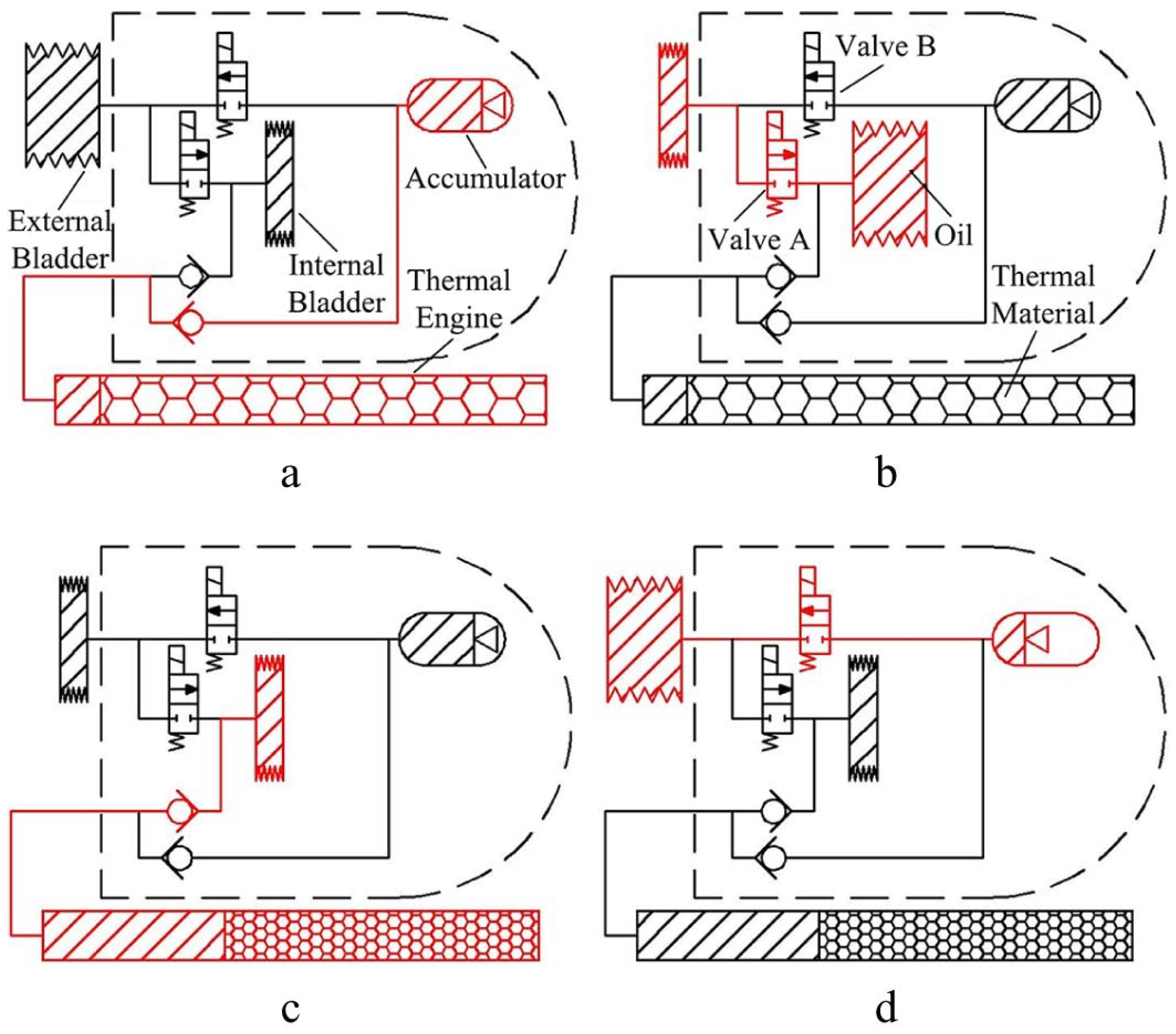
2.1. Working Principle

The “Petrel” underwater thermal vehicle is shown in Figure 1. It includes vehicle body and thermal engine. The functionality of the thermal engine is to harvest ocean thermal energy, and transform it into hydraulic potential energy which can be easily utilized. Compared with the conventional way of storing heat, this type of vehicle utilizes the volume difference between solid and liquid conditions of PCM to harvest thermal energy [43]. The underwater thermal vehicle working principle is shown in Figure 2 [44].
  • The vehicle initially drift on the sea surface, as shown in Figure 2a. Because of the high temperature of seawater, the PCM in the thermal machine is in liquid state. At this stage the working fluid is stored in the external bladder.
  • When the vehicle is prepared to dive, as shown in Figure 2b. The solenoid valve is opened, and the working fluid flows from the external bladder to the internal bladder. The volume of the vehicle is reduced, resulting in less buoyancy than gravity, and the vehicle sails to the deep ocean. When the vehicle sails to the deep sea, as shown in Figure 2c, the PCM solidifies and shrinks, causing a negative pressure in the thermal engine. Then the transfer fluid in the internal bladder flows into the thermal engine under this pressure difference.
  • When the vehicle is ready to ascend from the deep sea to the surface of the ocean, the channel in the solenoid valve that connects the accumulator to the external bladder is opened, as shown in Figure 2d. The working fluid stored in the accumulator flows into the external bladder. As a result, the volume of the vehicle increases, which causes the buoyancy force to be higher than gravity, and the vehicle sails upward.
  • When the vehicle dives up to warmer waters, the temperature around it gets higher. As a consequence, the PCM transforms from solid into liquid and expands. The working fluid in the thermal engine is then compressed into the accumulator for energy storage. When the PCM is completely melted, the thermal vehicle will return to the initial state shown in Figure 2a for the next cycle.

2.2. Mathematical Model

The schematic diagram of the vehicle and the coordinate system are shown in Figure 3. In accordance with Fossen’s definition, the underwater thermal vehicle dynamics are described in this paper under two reference coordinate systems [45]: The coordinate body reference and inertial coordinate reference. The coordinate body reference is fixed to the vehicle, with the floating center position as the coordinate origin and the X-axis as the direction of the vehicle’s axis. The inertial coordinate reference is the geodetic coordinate system. It records the global movement of the vehicle. Due to the non-linearity of the underwater vehicle itself and the uncertainty of its environment [46], the following assumptions are required before building the mathematical model to facilitate the design of the controller.
  • The center of buoyancy in a thermal vehicle can be considered to be constant. Buoyancy can be alternately reduced or increased by its buoyancy adjustment system while maintaining a nearly constant overall vehicle mass. The system decreases or increases the buoyancy to achieve a descending or ascending motion of the vehicle in the ocean;
  • The change of mass distribution in the vehicle caused by the actuator motion is neglected. The mass of the center of gravity adjustment is very small, and it can be neglected compared to the total mass and length of the thermal vehicle;
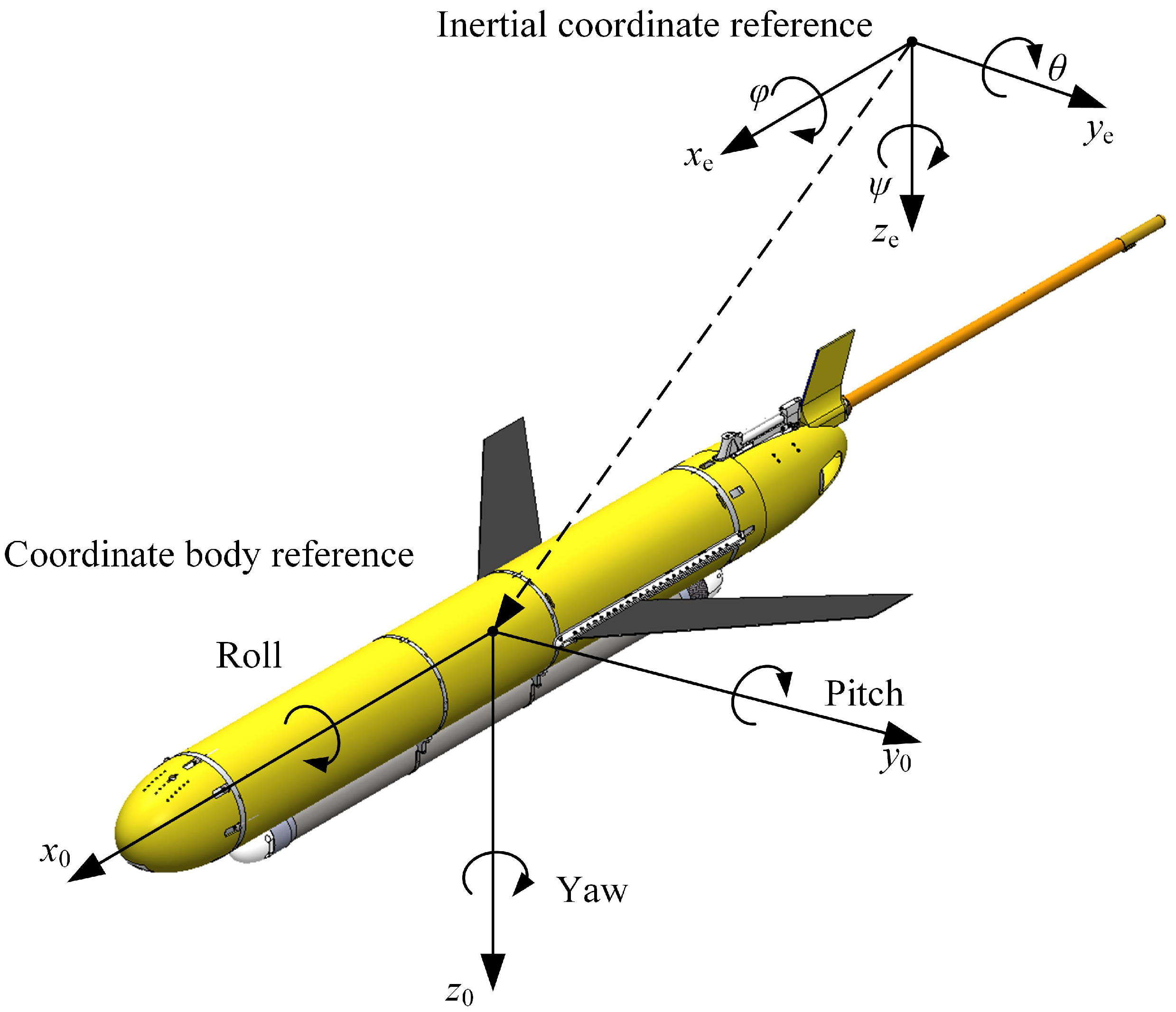
  • Since the underwater vehicle is rarely adjusted in the roll and yaw directions. Therefore, only considering the motion of the underwater vehicle in the vertical plane;
  • Pitching angle θ range from π / 2 to π / 2 .
Based on the above assumptions, the mathematical model of the underwater thermal vehicle in the vertical plane can be described as follows [41,47]:
θ ˙ = ω 2 ω 2 . = 1 J 2 + r m s s ( ( m f 3 m f 1 ) v 1 v 3 + M f c ( r m s ( v 1 + s ω 2 ) + s P P 3 ) ω 2 m s g ( r sin ( θ ) + s cos ( θ ) ) r ( P P 3 ω 2 m s v 3 ω 2 m s r ω 2 2 ) s u s ˙ = 1 m s ( P P 3 v 3 r ω 2 ) P ˙ P 3 = u
where θ is pitch angle, ω 2 is velocity of pitching, J 2 is moment of inertia of the vehicle, and M f c is the hydrodynamic coefficient of the vehicle, its expression is shown in Equation (2). v 1 and v 3 respectively represent the axial, longitudinal velocity of underwater vehicle, m f 1 , m f 3 are added mass and slider mass, m s 3 is the stationary body mass of vehicle, P P 3 is the vertical moment of inertia. s and r are the position of vehicle in the vertical plane, in which the slider is fixed in the axial movement position, so r can be set as a constant. g is gravity acceleration, u is the power for the axial movement of the slider, which is obtained from the motor driving the movement of the slider.
M f c = K M 0 + K M α v 1 2 + v 3 2
where the K M 0 and K M are constant coefficients. α is the trim angle. This model is a standard one, derived using airfoil theory and potential flow calculations and then verified using experimental observations [48].
Generally, there are natural limits on the linear and angular velocities of an underwater thermal vehicle. Therefore, the following boundary conditions can be defined:
ω 2 m i n ω 2 ω 2 m a x
where ω 2 m i n and ω 2 m a x are the upper and lower bounds of the angular velocity of underwater vehicles, and both can be obtained from the prototype design.
To facilitate controller design, the underwater thermal vehicle vertical plane dynamics as described in Equations (1) and (2) can be represented by the following nonlinear discrete state equation:
x ( t + 1 ) = f t ( x ( t ) ) + Bu ( t ) y ( t ) = C x ( t )
where x ( t ) = [ θ ( t ) , ω 2 ( t ) , s ( t ) , P P 3 ( t ) , ] T , B = [ 0 , s J 2 + r m s s , 0 , 1 ] T ,
f t x t = ω 2 1 J 2 + r m s s m f 3 m f 1 v 1 v 3 + K M 0 + K M α v 1 2 + v 3 2 r m s v 1 + s ω 2 + s P P 3 ω 2 m s g ( r sin ( θ ) + s cos ( θ ) ) r P P 3 ω 2 m s v 3 ω 2 m s r ω 2 2 1 m s P P 3 v 3 r ω 2 0 .
Because we only care about the change of the pitch angle θ ˙ , y t is set to θ ˙ . Therefore, C is set as [ 1 , 0 , 0 , 0 ] T .

3. Controller Design

3.1. Linearization of the Mathematical Model

To facilitate the expression, the state variables of the system can be defined as follows:
x 1 ( t ) = θ ˙ x 2 ( t ) = ω ˙ 2 x 3 ( t ) = s ˙ x 4 ( t ) = P ˙ P 3
where the x 1 ( t ) , x 2 ( t ) , x 3 ( t ) , x 4 ( t ) are each expressed as follows:
x ( t ) = x 1 ( t ) x 2 ( t ) x 3 ( t ) x 4 ( t ) T .
Since the thermal vehicle runs slowly and works in a relatively single state, it can be generally considered to work only near its working point. Setting the working point of the vehicle as [ θ c , ω 2 c , s c , P P 3 c ] , then the nonlinear model shown in Equation (3) can be linearized around its working point to obtain the following linear model:
x 1 ( t ) = x 2 ( t 1 ) x 2 ( t ) = a 21 x 1 ( t 1 ) + a 22 x 2 ( t 1 ) + a 23 x 3 ( t 1 ) + a 24 x 4 ( t 1 ) + b 2 u ( t 1 ) x 3 ( t ) = a 32 x 2 ( t 1 ) + a 34 u ( t 1 ) x 4 ( t ) = u ( t 1 ) .
The coefficients in Equation (7) are shown in Equations (8)–(14), respectively.
a 21 = g m s ( r cos ( θ c ) s c sin ( θ c ) ( J 2 + r m s s c )
a 22 = s c P P 3 c r ( m s v 3 P P 3 c + 2 m s r ω 2 c ) + m s r ( 2 ω 2 c s c + v 1 ) ( J 2 + r m s s c )
a 23 = m s r J 2 + r m s s c K M 0 + K M α v 1 2 + v 3 2 + s c u c r ( P P 3 c ω 2 c + m s v 3 ω 2 c + m s r ω 2 c 2 ) + m s g ( r sin ( θ c ) + s cos ( θ c ) ) + ( m f 3 m f 1 v 1 v 3 ) ω 2 c ( P P 3 c + m s r ω 2 c ) J 2 + r m s s c
a 24 = ω 2 c ( r + s c ) J 2 + r m s s c
a 32 = r
a 34 = 1 m s
b 2 = s c J 2 + r m s s c .
In order to facilitate the design of discrete controllers, in this paper, we describe the discrete-time system by introducing the delay operator q 1 . For example, the state φ t 1 at t 1 moments can be described as q 1 φ t . Thus, Equation (7) can be described as:
1 a 22 q 1 a 21 + a 23 a 32 q 2 x 1 ( t ) = q 1 a 23 a 34 + a 24 q 1 + b 2 q 2 u ( t ) .
Let the expressions of A ( q 1 ) , B ( q 1 ) respectively be in the form shown in Equations (16) and (17), then Equation (15) can be rewritten as in Equation (18).
A q 1 = 1 a 22 q 1 a 21 + a 23 a 32 q 2
B q 1 = b 2 q 1 + a 23 a 34 + a 24 q 2
y ( t ) = x 1 ( t ) = q 1 B ( q 1 ) A ( q 1 ) u ( t ) .
Assuming that the disturbance of the ocean environment is p ( t ) and it directly acts on the output of the underwater thermal vehicle, then the mathematical model of the underwater thermal vehicle with consideration of the environmental disturbance can be written as:
y ( t ) = q 1 B ( q 1 ) A ( q 1 ) u ( t ) + p ( t ) .
Generally, the environmental random disturbance signal can be expressed as a discrete-time white noise signal as input and the output signal of some structural filter. Its general expression is shown in the following form (Auto Regressive and Moving Average: ARMA) [49]:
p ( t ) = N ( q 1 ) D ( q 1 ) e ( t )
where e ( t ) is the normalized discrete-time white noise signal. N ( q 1 ) and D ( q 1 ) are coprime polynomials in q 1 , with degrees n N and n D . Since ocean disturbances are generally bandwidth limited, the roots of D ( q 1 ) are on the units circle [50]. The energy of the disturbance is represented by D ( q 1 ) , the contribution of the N ( q 1 ) is very weak and can be neglected.
By taking Equation (20) into Equation (19), the ARMAX model of the ocean thermal underwater vehicle can be obtained as shown in Equation (21).
y ( t ) = q 1 B ( q 1 ) A ( q 1 ) u ( t ) + N ( q 1 ) D ( q 1 ) e ( t ) .

3.2. Controller Design for Disturbances with Known Parameters

3.2.1. RS Controller Structure

The polynomial controller (RS) controller is a polynomial output feedback controller structure with polynomials R ( q 1 ) and S ( q 1 ) . Assume that the relationship between the controller structure polynomials R ( q 1 ) and S ( q 1 ) and the system input u ( t ) and output y ( t ) is shown as follows [39]:
S ( q 1 ) u ( t ) = R ( q 1 ) y ( t )
where S ( q 1 ) and R ( q 1 ) ) is the controller structure which can be expressed as:
S ( q 1 ) = 1 + s 1 q 1 + + s n s q n s
R ( q 1 ) = r 0 + r 1 q 1 + + r n r q n r
where n s is the degree of the polynomial S ( q 1 ) and n r is the degree of the polynomial R ( q 1 ) .
By bringing Equation (22) into Equation (21), the relationship between the output and the disturbances of the underwater thermal vehicle can be obtained, as follows:
y ( t ) = S ( q 1 ) N ( q 1 ) A ( q 1 ) S ( q 1 ) + q 1 B ( q 1 ) R ( q 1 ) D ( q 1 ) e ( t ) = S ( q 1 ) N ( q 1 ) p ( q 1 ) D ( q 1 ) e ( t )
where:
p ( q 1 ) = A ( q 1 ) S ( q 1 ) + q 1 B ( q 1 ) R ( q 1 ) .
In order to be able to asymptotically stabilize the closed-loop polynomial p ( q 1 ) of the system, S ( q 1 ) can be pre-designed to contain the disturbance term, which with the following form:
S ( q 1 ) = S ( q 1 ) D ( q 1 )
where S ( q 1 ) is part of the controller S ( q 1 ) that is to be designed.
Equation (26) defines the closed-loop poles of the system and it also determines the dynamic response behavior of the system. The order relationship of each polynomial in Equation (26) are shown as follows:
n p n A + n B + d 1 n S = n B + d 1 n R = n A 1 .
In order to obtain a good anti-disturbance performance for the thermal vehicle, the method of pole assignment is used to optimize the positioning of the closed-loop poles of Equation (18).

3.2.2. Pole Assignment

The H∞ method is utilized to obtain the optimal closed-loop pole position. To implement this idea, this paper rewrites Equation (11) in the form of the following linear time-invariant equation:
y ^ ( t ) y ^ ( t 1 ) = a 22 a 21 + a 23 a 32 1 0 y ^ ( t 1 ) y ^ ( t 2 ) + b 2 a 23 a 34 + a 24 0 0 u t 2 u t 3
y ( t ) = 1 0 y ^ ( t ) y ^ ( t 1 ) + p t
Let:
A 1 = a 22 a 21 + a 23 a 32 1 0
B 1 = b 2 a 23 a 34 + a 24 0 0
C 1 = 1 0
φ ^ ( t + 1 ) = y ^ ( t ) y ^ ( t 1 ) .
Then, Equation (29) can be abbreviated as the following form:
φ ^ ( t + 1 ) = A 1 φ ^ ( t ) + B 1 u ( t 2 ) y ( t ) = C 1 φ ^ ( t ) + p ( t )
The following state feedback control law is adopted:
u ( t ) = K φ ^ ( t ) .
For Equation (35), the following theorem can be obtained.
Theorem 1.
For the system Equation (35), under the condition of without considering the interference of output, if there is a definite symmetric matrix, which make the following linear matrix inequality established:
M 0 M 0 A B N 0 * M 0 + Φ M 0 C T * * Φ < 0 .
Then, the state feedback control gain K can be obtained, which is as follows.
K = N 0 M 0 1 .
Proof .
By substituting Equation (36) into (35), the closed-loop system is obtained as:
φ ^ ( t + 1 ) = A φ ^ ( t ) BK φ ^ ( t 2 ) .
Denoting the following Lyapunov function:
V ( t ) = φ ^ T ( t ) P φ ^ ( t ) + i = 1 2 φ ^ T ( t i ) M φ ^ ( t i ) .
The following equation can be obtained by differentiating Equation (41):
V ( t ) = V ( t + 1 ) V ( t ) = φ ^ T ( t + 1 ) P φ ^ ( t + 1 ) + i = 1 2 φ ^ T ( t i + 1 ) M φ ^ ( t i + 1 ) φ ^ T ( t ) P φ ^ ( t ) i = 1 2 φ ^ T ( t i ) M φ ^ ( t i ) = ( A φ ^ ( t ) + B K φ ^ ( t 2 ) ) T P ( A φ ^ ( t ) + B K φ ^ ( t 2 ) ) φ ^ T ( t ) ( P M ) φ ^ ( t ) φ ^ T ( t 2 ) M φ ^ ( t 2 ) .
Rewrite V ( t ) + y T ( t ) y ( t ) in equivalent matrix form as:
φ ^ T ( t ) φ ^ T ( t 2 ) T Θ φ ^ T ( t ) φ ^ T ( t 2 )
where Θ = A T PA P + M + C T C A T PBK * ( BK ) T PBK M .
In accordance with Schur-Complementary principle, Θ < 0 can be represented as follows:
P 1 A BK * P + M C T * * M < 0 .
Equation (43) is transformed by using pre-multiplication and post-multiplication in the matrix d i a g ( I , P 1 , P 1 ) , letting M 0 = P 1 , N 0 = KP 1 = K M 0 , Φ = PM P 1 , to obtain Equation (38).
Suppose that the state feedback gain obtained by solving using Equation (38) is shown as follows:
K = k 11 k 12 k 21 k 22 .
Bringing Equation (44) to Equation (29), the following expression can be obtained:
y ^ ( t ) y ^ ( t 1 ) = a 22 a 21 + a 23 a 32 1 0 y ^ ( t 1 ) y ^ ( t 2 ) + b 2 a 23 a 34 + a 24 0 0 k 11 k 12 k 21 k 22 y ^ ( t 3 ) y ^ ( t 4 ) .
Expanding the above formula, the following expression can be obtained:
y ^ ( t ) = a 22 y ^ ( t 1 ) a 21 + a 23 a 32 y ^ ( t 2 ) + b 2 k 11 + k 21 a 23 a 34 + a 24 y ^ ( t 3 ) + b 2 k 12 + k 22 a 23 a 34 + a 24 y ^ ( t 4 ) .
Transforming the above equation in the form of the matrix, we can obtain the following structure.
φ 3 ( t ) = Ψ φ 3 ( t 1 ) .
In which:
φ 3 ( t ) = y ^ ( t ) y ^ ( t 1 ) y ^ ( t 2 ) y ^ ( t 3 ) T
Ψ = a 22 a 21 + a 23 a 32 b 2 k 11 + k 21 a 23 a 34 + a 24 b 2 k 12 + k 22 a 23 a 34 + a 24 1 0 0 0 0 1 0 0 0 0 1 0
Specifically, Ψ is the autonomic state matrix of the closed-loop system (35), and its eigenvalues are the closed-loop desired poles obtained by employing the H configuration.
Suppose that the eigenroots obtained by solving the characteristic roots for Ψ are p 1 , p 2 , p 3 , p 4 . Then the closed-loop expectation polynomial p ( q 1 ) of the system can be expressed as follows:
p ( q 1 ) = 1 + p 1 q 1 + p 2 q 2 + p 3 q 3 + p 4 q 4 .

3.2.3. Disturbance Suppression Controller Design

When p ( q 1 ) is determined, it is necessary to design both R ( q 1 ) and S ( q 1 ) . In this paper, we adopt the Youla–Kucera parametrization (Q-parametrization) of all stable controllers [51], the controller polynomials R ( q 1 ) and S ( q 1 ) can be rewritten as the following form [52]:
R ( q 1 ) = R 0 ( q 1 ) + A ( q 1 ) Q ( q 1 )
S ( q 1 ) = S 0 ( q 1 ) q 1 B ( q 1 ) Q ( q 1 )
where Q ( q 1 ) is the controller parameter with degree n Q , and has the following form [52]:
Q ( q 1 ) = q 0 + q 1 q 1 + + q n Q q n Q .
The central controller R 0 ( q 1 ) and S 0 ( q 1 ) can be computed by solving the following equation:
P ( q 1 ) = A ( q 1 ) S 0 ( q 1 ) + q 1 B ( q 1 ) R 0 ( q 1 ) .
In order to solve Q ( q 1 ) , it is necessary to solve the following dropfantine equation:
S 0 ( q 1 ) = S ( q 1 ) D ( q 1 ) + q 1 B ( q 1 ) Q ( q 1 )
where D ( q 1 ) , B ( q 1 ) , and S 0 ( q 1 ) are known. The polynomial formulation of Q ( q 1 ) and S ( q 1 ) can be obtained by solving Equation (55). Taking them into Equations (51) and (52), we can obtain the R S controller.

3.3. Controller Design for Disturbances with Unknown Parameters

During the above controller design process, the structure of the disturbance signals is already known. However, in the real ocean environment, the underwater thermal vehicle’s motion mainly receives the influence of factors such as currents and winds. The velocity changes of such disturbances are generally more fractionally slow, but their structural parameters usually cannot be known beforehand. In this case, the disturbance rejection control algorithm proposed in Section 2.2 for the disturbed structure and the understood parameters is not sufficient. In this case, in order to improve the disturbance rejection effect of the system and improve the response speed. The model for identifying the ocean disturbance signal parameters is preferred in this section to transform the disturbance model with unknown parameters into the known one. Based on this, the R S controller designed in Section 2.2 of this paper is used to suppress the disturbance signals obtained from the discrimination.
Assume that the unknown disturbance signal encountered by the underwater thermal vehicle in operation is of a sinusoidal form and that the disturbance is of a single frequency at any moment. Then the continuous disturbance signal:
p t = A 0 t sin ω t
where A 0 is the unknown amplitude of the disturbance signal and ω is the unknown disturbance frequency. By discretizing the above equation, the discrete model of the disturbance signal can be expressed as follows:
p t = n 0 + n 1 q 1 1 + d 1 q 1 + d 2 q 2 e t = N q 1 D q 1 e t
where n 0 , n 1 , d 1 , and d 2 are the unknown parameters of the disturbance.
Bringing Equation (57) into Equation (21), the following results can be obtained:
A ( q 1 ) D ( q 1 ) y ( t ) = q 1 B ( q 1 ) D ( q 1 ) u ( t ) + A ( q 1 ) N ( q 1 ) e ( t ) .
Then, we can reformulate Equation (58) into the following format:
y t = y t 1 + a 22 y t 2 + a 21 + a 23 a 32 y t 3 + b 2 u t 3 + a 23 a 34 + a 24 u t 4 y t 2 + a 22 y t 3 + a 21 + a 23 a 32 y t 4 + b 2 u t 4 + a 23 a 34 + a 24 u t 5 a 22 e t 1 a 21 + a 23 a 32 e t 2 a 22 e t 2 a 21 + a 23 a 32 e t 3 T d 1 d 2 n 0 n 1 + y t 1 y t 2 u t 2 u t 3 T a 1 a 2 b 1 b 2 + n 0 e t .
Let Γ 1 t to be set as:
y t 1 + a 22 y t 2 + a 21 + a 23 a 32 y t 3 + a 23 a 34 + a 24 u t 3 + b 2 u t 4 y t 2 + a 22 y t 3 + a 21 + a 23 a 32 y t 4 + a 23 a 34 + a 24 u t 4 + b 2 u t 5 a 22 e t 1 a 21 + a 23 a 32 e t 2 a 22 e t 2 a 21 + a 23 a 32 e t 3 ;
χ to be set as d 1 d 2 n 0 n 1 T ; Γ 2 is to be set as y t 1 y t 2 u t 2 u t 3 T ;
η 2 to be set as a 22 a 21 + a 23 a 32 b 2 a 23 a 34 + a 24 T ; ω t is to be set as n 0 e t . Then the Equation (59) can be abbreviated to the following form:
y t = Γ 1 T t χ + Γ 2 T t η 2 + ω t .
For the sake of calculation, in this paper, we take z ( t ) as y t Γ 2 T t η 2 . That is, Equation (60) can be transformed into the standard parameter identification system as follows:
z t = Γ 1 T t χ + ω t .
In this paper, the parameter vector χ can be solved by the forgetful factor least squares method. Before solving, since ω t is not measurable, only its estimated value ω ^ t can be used instead. The estimate of ω ^ t can be obtained by the following equation:
ω ^ t = z t z ^ t = z t Γ ^ 1 T t χ ^ t
where Γ ^ 1 is set as:
y t 1 + a 22 y t 2 + a 21 + a 23 a 32 y t 3 + a 24 + a 23 a 34 u t 3 + b 2 u t 4 y t 2 + a 22 y t 3 + a 21 + a 23 a 32 y t 4 + a 24 + a 23 a 34 u t 4 + b 2 u t 5 a 22 e ^ t 1 a 21 + a 23 a 32 e ^ t 2 a 22 e ^ t 2 a 21 + a 23 a 32 e ^ t 3 .
The performance indicators is designed as:
J = t = 1 L λ L t z ( t ) Γ ^ 1 T t χ ^ t 2
where λ is the forgetting factor ( 0 < λ 1 ). L is the observation time.
Aiming at the target function shown in Equation (63), the following forgetting factor least squares algorithm can be used to estimate χ ^ t [53]:
χ ^ ( t ) = χ ^ ( t 1 ) + K ( t ) z ( t ) Γ ^ 1 T t χ ^ t K ( t ) = P ( t 1 ) Γ ^ 1 T t λ + Γ ^ 1 T t P ( t 1 ) Γ ^ 1 t P ( t ) = 1 λ ( I K ( t ) Γ ^ 1 T t ) P ( t 1 ) .
With Equation (64), we can obtain the estimated value of χ at time t, that is, the unknown disturbance signal can be identified as the known one. Then, we can use the control law designed in Section 2.2 of this paper to suppress the external disturbance. The detailed algorithm steps are shown as follows:
(1)
Solve S 0 ( q 1 ) , R 0 ( q 1 ) by the pre-set poles P ( q 1 ) , utilizing Equation (54).
(2)
Obtain ω ^ t by outputting y ( t + 1 ) ,applying control u ( t ) , via Equation (62).
(3)
Estimate the χ ^ ( t ) related perturbation parameters (i.e., the parameters of the polynomial D ( q 1 ) ) with the parameter estimation Equation (64).
(4)
The control parameter Q ( q 1 ) can be obtained by solving the equation of the dropfan diagram by bringing D ( q 1 ) obtained in the previous step into Equation (55).
(5)
Bring the S 0 ( q 1 ) and R 0 ( q 1 ) obtained from the first step and the Q ( q 1 ) obtained from the fourth step into Equations (51) and (52), and then the controller parameters can be solved.

4. Simulation Results and Discussion

In order to verify the control algorithm’s effectiveness, this section conducts a simulation of the controller proposed in this paper under Matlab/Simulink. The simulation parameters are shown in Table 1. Simultaneously, to compare and analyze the control effect of the RS controller, the PID controller with optimized and adjusted parameters is taken as a comparison. The control law of the proposed PID controller is shown as follows:
u PID t = 0.008294 θ r θ t 7.1307 θ r θ t d t + 0.00921 θ ˙ r θ ˙ t .
In this paper, three different cases are analyzed in this paper by individual cases. In case 1, the external interference is a single frequency sinusoidal interference with known structure and parameters. In case 2, the external interference is a single frequency sinusoidal interference, but the disturbance signal parameters are unknown. In case 3, the observed data of the current disturbance shown in the literature [3] is retrieved as the unknown external disturbance. The reference pitch angle θ r is taken as:
θ r t = 17 0 s t 2000 s θ r t = 17 2000 s < t 4000 s .
Case 1: The disturbance is sinusoidal and its form is shown as follows:
p ( t ) = A cos ( 2 π f t )
where A and f are the amplitude and frequency of the disturbance signal, respectively, and these parameters are known. For the achievement in simulation, let A = 1 . The frequencies f = 0.01 , 0.05 , 0.1 , 1 Hz are considered. The closed-loop desired pole P ( q 1 ) of the system obtained by the pole configuration method is shown in Equation (68). The RS controller obtained from this paper is as shown in Equation (69).
P q 1 = 1.0000 0.7417 q 1 + 0.2019 q 2
R q 1 = 0 . 0173 + 0 . 0138 q 1 + 0 . 0001 q 2 S q 1 = 1 . 0000 1 . 4679 q 1 0 . 3450 q 2 + 0 . 8129 q 3
The simulation results are shown in Figure 4 for different controllers, and the controller outputs are shown in Figure 5. This paper quantifies the 5% over-tuning time ( T s ) and steady-state error ( E s ) as indicators to validate the control algorithm’s effectiveness under different frequency conditions. The smaller these two performance indicators are, the better the disturbance suppression effect.
The 5% over-tuning time ( T s ) and steady-state errors ( E s ) of the different object for the vibration with different frequencies are shown in Table 2. As can be seen from Figure 4 and Table 2, the time to reach the set value with the RS controller is significantly shorter than the PID control strategy. This indicates that the dynamic tracking performance of the RS controller is better under the influence of different frequency disturbances. Besides, the steady-state error with RS controller is smaller when the disturbance frequency ranges between 0.01 Hz and 0.05 Hz. That is, the RS controller is more effective in disturbance suppression. However, when the frequency increases above 0.1 Hz, the control strategy cannot effectively suppress the disturbance. This indicates that the control algorithm proposed in this paper is effective in suppressing low-frequency sinusoidal disturbances. In other words, the effectiveness of the RS controller for suppressing low-frequency disturbances can be verified.
Besides the disturbance suppression effect, the energy consumption level of the actuator also needs to be considered. The actuator’s output force directly reflects the level of energy consumption required by the underwater vehicle to achieve the desired control effect. The higher the value, the higher the level of energy consumption.
Figure 5 shows the value of the controller output force. As can be seen, compared with the PID control strategy, the RS controller needs to adjust the control force’s magnitude and direction u ( t ) in real-time to suppress the environmental disturbances. When the disturbance frequency is less than 0.05 Hz, the frequency and magnitude of the change in the control force u ( t ) are slightly greater than the PID controller’s output force, but the difference is negligible. The level of energy consumption using the RS controller can still reach a relatively low level at this time. When the disturbance frequency is greater than 0.1 Hz, the control force’s frequency and amplitude u ( t ) increase significantly compared to the traditional PID control strategy, which means that the actuator needs to consume more energy to meet the control force demand.
Case 2: The disturbance is set as a segmented unknown sinusoidal disturbance and the expression is given as follows:
p t = A 1 cos 2 π f 1 t t 0 , 1000 2000 , 3000 A 2 cos 2 π f 2 t t 1000 , 2000 3000 , 4000
where A 1 , A 2 are the unknown amplitude parameters set to 0.5 and 2.0 respectively in the simulation. f 1 , f 2 are the unknown frequencies, which are set to 0.05 Hz, 0.01 Hz respectively in the simulation. In the simulation, the sampling period T s is 1 s.
The estimated values of external disturbances are shown in Figure 6. As can be seen, concerning the estimation of the frequency, the method described in this paper can perform good tracking and estimating of the disturbance’s frequency. In terms of amplitude estimation, when t 0 , 1000 2000 , 3000 s, the estimation result is 0.407° by the parameter identification method, which is slightly lower than the predefined value (0.5°). The estimation error is about 18.6%. When t 1000 , 2000 3000 , 4000 s, the estimated result is 1.63° by the parameter identification method, which is slightly lower than the predefined value (2°). The estimation error is about 18.5%. To summarize, the disturbance estimation method proposed in Section 2 of this paper is effective.
The control effect of the pitch angle θ is shown in Figure 7. When t 0 , 1000 2000 , 3000 s, for the RS controller, the T s , and E s are 57 s and 0.26°, respectively; for the PID controller, the T s and E s are 910 s and 0.97°, respectively. When t 1000 , 2000 3000 , 4000 s, the E s with the RS controller and PID controller are 0.11° and 2.08°, respectively. This result indicates that the RS controller has a significant advantage in the disturbance suppression effect and response time. Besides, when the disturbance changes suddenly, the pitch angle varies, as shown in the partial plot in Figure 7. As can be seen, the pitch angle θ with the RS controller can quickly capture this change and correct it. The adjustment rate of the PID controller is slightly slower. The above results indicate that the controller can effectively reject the disturbance of unknown frequency and amplitude. Besides, the simulation results also show that the rejection effect decreases as the disturbance frequency increases.
Figure 8 shows the controller output force in Case 2. Similar to Case 1, the RS controller requires real-time adjustment of the control force’s magnitude and direction. Hence, its energy consumption level shows an increase compared to the PID controller, but the difference is negligible. As can be seen from the partial diagram in Figure 8, the RS controller output force can be adjusted immediately when the disturbance appears to change to achieve disturbance suppression. Compared with RS, the PID control algorithm shows a weaker real-time adjustment capability.
Case 3: In order to evaluate the effectiveness of the control algorithm proposed by this paper in the case of a real ocean environment, the waves measured in the literature [3] were extracted as the disturbance signal, as shown in Figure 9. It can be seen from the figure that the wave signal state information is unknown and the frequency varies with time.
The simulation results of the pitch angle θ are shown in Figure 10. As can be seen, the pitch angle θ with the RS controller has more minor fluctuations under simulated waves’ interference conditions. The steady-state error of the whole process is less than 0.73°. The pitch angle θ with the PID control strategy shows fluctuation with the fluctuation of the sea current, and the steady-state error is up to 2.42° when it reaches the set value. Compared with the PID control strategy, the adaptive RS control strategy proposed in this paper has significant advantages in suppressing disturbances. The effectiveness of this control strategy for ocean environment disturbance suppression has been verified.
Figure 11 shows the value of the controller output force. As can be seen, the control force is about 2 N, and it needs to change following the disturbance signal. Compared with the PID control strategy, while the disturbance rejection effect is improved, its control energy consumption also increases.

5. Conclusions

An adaptive control strategy based on the internal model principle was proposed for the ocean thermal underwater vehicle’s pitch angle control problem. Simulation experiments verified the effectiveness of the designed controller, and the following conclusions could be drawn:
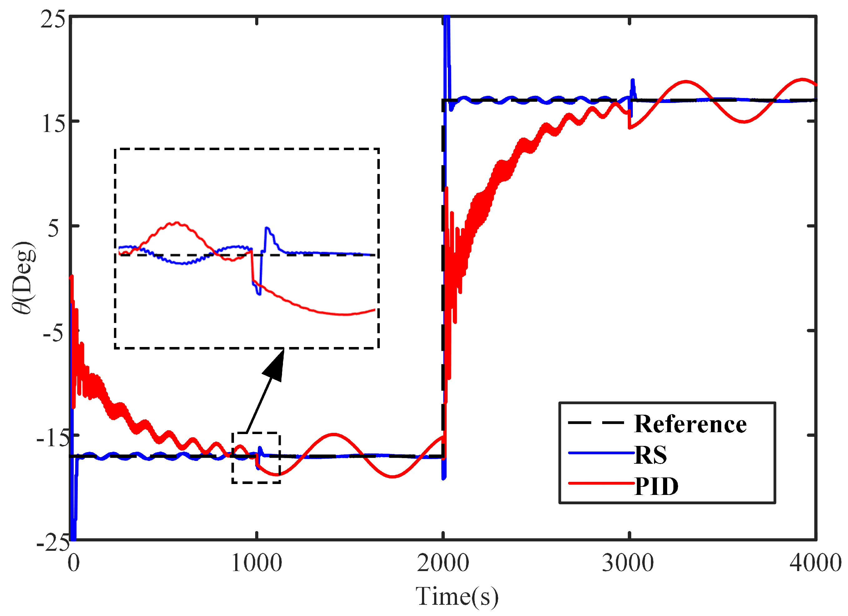
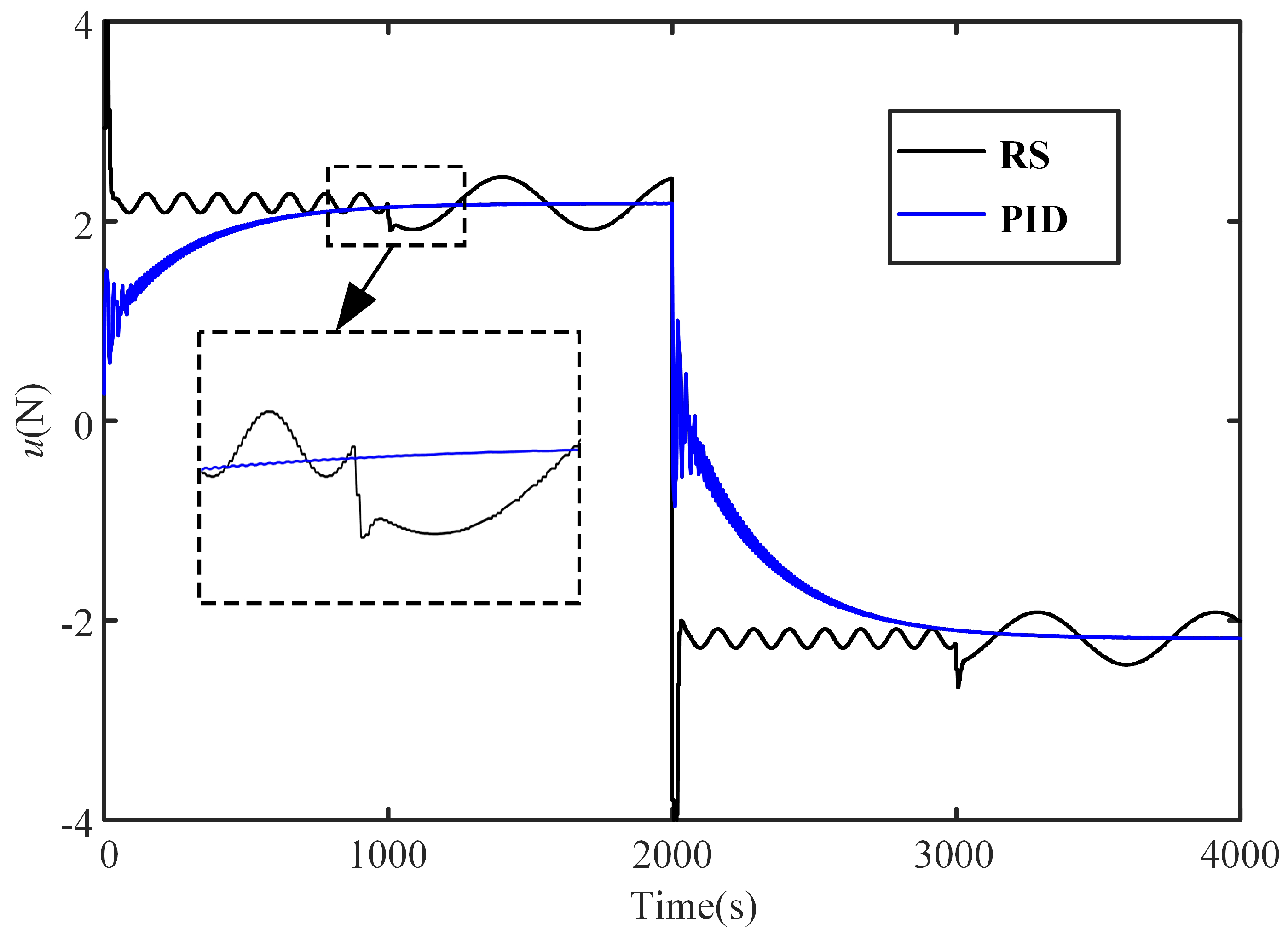
  • For known parameters and bounded external disturbance, this controller could compensate the disturbance by pre-setting the control parameters using the internal model principle and parameterization method. The simulation results showed that this approach was particularly effective in low and medium frequency bands;
  • In the case where the parameters of perturbation were unknown, in this paper, firstly, we used the parameter identification method to estimate the environmental disturbances. This approach could transform the disturbance with unknown parameters into a known one, which the R S type controller could then suppress. Simulation analysis with unknown parameters and time-varying wave signals as disturbances showed that the proposed strategy was effective.
The adaptive digital control algorithm designed in this paper was simple in structure. It could be applied to the precise measurement of specific areas that need to be attended to. Considering the economic and observable accuracy, the underwater thermal vehicle with RS controller should operate in the following form:
  • When the vehicle needs to reach a location quickly or when the trial area’s sea conditions are good, this controller will be turned off, and only the PID will be used to control the pitch angle;
  • When the environmental disturbances (such as currents, waves, etc.) are significant, which significantly affects the vehicle’s observation in the focused region, this controller can be turned on to reduce the impact of environmental disturbances on it. The controller can be turned on to minimize the effect of environmental disturbances on the vehicle and make the vehicle sail more smoothly, thus achieving high accuracy observation.

Author Contributions

G.W.: Conceptualization, Formal analysis, Data curation, Writing—original draft. Y.Y.: Conceptualization, Writing—original draft. S.W.: Conceptualization, Methodology, Project administration. All authors have read and agreed to the published version of the manuscript.

Funding

This research was funded by National Natural Science Foundation of China (Grant Nos. 52006155).

Institutional Review Board Statement

Not applicable.

Informed Consent Statement

Not applicable.

Data Availability Statement

Data sharing not applicable.

Conflicts of Interest

The authors declare that they have no known competing financial interests or personal relationships that could have appeared to influence the work reported in this paper.

References

  1. Wakita, N.; Hirokawa, K.; Ichikawa, T.; Yamauchi, Y. Development of autonomous underwater vehicle (AUV) for exploring deep sea marine mineral resources. Mitsubishi Heavy Indu. Tech. Rev. 2010, 47, 73–80. [Google Scholar]
  2. Fernández-Perdomo, E.; Cabrera-Gámez, J.; Hernández-Sosa, D.; Isern-González, J.; Domínguez-Brito, A.C.; Redondo, A.; Coca, J.; Ramos, A.G.; Fanjul, E.Á.; García, M. Path planning for gliders using Regional Ocean Models: Application of Pinzón path planner with the ESEOAT model and the RU27 trans-Atlantic flight data. In Proceedings of the OCEANS’10 IEEE SYDNEY, Sydney, NSW, Australia, 24–27 May 2010; pp. 1–10. [Google Scholar]
  3. Fernández, D.C.; Hollinger, G.A. Model predictive control for underwater robots in ocean waves. IEEE Robot. Automat. Lett. 2017, 2, 88–95. [Google Scholar] [CrossRef]
  4. Wang, G.; Yang, Y.; Wang, S.; Zhang, H.; Wang, Y. Efficiency analysis and experimental validation of the ocean thermal energy conversion with phase change material for underwater vehicle. Appl. Energy 2019, 248, 475–488. [Google Scholar] [CrossRef]
  5. Wang, G.; Yang, Y.; Wang, S. Ocean thermal energy application technologies for unmanned underwater vehicles: A comprehensive review. Appl. Energy 2020, 278, 115752. [Google Scholar] [CrossRef]
  6. Singh, Y.; Bhattacharyya, S.; Idichandy, V. CFD approach to steady state analysis of an underwater glider. In Proceedings of the 2014 Oceans-St. John’s, St. John’s, NL, Canada, 14–19 September 2014; pp. 1–5. [Google Scholar]
  7. Singh, Y.; Bhattacharyya, S.; Idichandy, V. CFD approach to modelling, hydrodynamic analysis and motion characteristics of a laboratory underwater glider with experimental results. J. Ocean Eng. Sci. 2017, 2, 90–119. [Google Scholar] [CrossRef]
  8. Yang, C.; Peng, S.; Fan, S.; Zhang, S.; Wang, P.; Chen, Y. Study on docking guidance algorithm for hybrid underwater glider in currents. Ocean Eng. 2016, 125, 170–181. [Google Scholar] [CrossRef]
  9. Sitaba, A.I.; Trilaksono, B.R.; Hidayat, E.M.I.; Sagala, M.F. Communication system and visualization of sensory data and HILs in autonomous underwater glider. In Proceedings of the 6th International Conference on Electrical Engineering and Informatics (ICEEI), Langkawi, Malaysia, 25–27 November 2017; pp. 1–6. [Google Scholar]
  10. Mina, T.; Singh, Y.; Min, B.C. Maneuvering Ability-Based Weighted Potential Field Framework for Multi-USV Navigation, Guidance, and Control. Mar. Technol. Soc. J. 2020, 54, 40–58. [Google Scholar] [CrossRef]
  11. Xue, D.Y.; Wu, Z.L.; Wang, Y.H.; Wang, S.X. Coordinate control, motion optimization and sea experiment of a fleet of Petrel-II gliders. Chin. J. Mech. Eng. 2018, 31, 1–15. [Google Scholar] [CrossRef] [Green Version]
  12. Leonard, N.E.; Paley, D.A.; Lekien, F.; Sepulchre, R.; Fratantoni, D.M.; Davis, R.E. Collective motion, sensor networks, and ocean sampling. Proc. IEEE 2007, 95, 48–74. [Google Scholar] [CrossRef] [Green Version]
  13. Chocron, O.; Vega, E.; Benbouzid, M. Evolutionary dynamic reconfiguration of AUVs for underwater maintenance. In Marine Robotics and Applications; Springer: Berlin/Heidelberg, Germany, 2018; pp. 137–178. [Google Scholar]
  14. Webb, D.C.; Simonetti, P.J.; Jones, C.P. SLOCUM: An underwater glider propelled by environmental energy. IEEE J. Ocean. Eng. 2001, 26, 447–452. [Google Scholar] [CrossRef]
  15. Huang, Z.; Liu, Y.; Zheng, H.; Wang, S.; Ma, J.; Liu, Y. A self-searching optimal ADRC for the pitch angle control of an underwater thermal glider in the vertical plane motion. Ocean Eng. 2018, 159, 98–111. [Google Scholar] [CrossRef]
  16. Joe, H.; Kim, M.; Yu, S.C. Second-order sliding-mode controller for autonomous underwater vehicle in the presence of unknown disturbances. Nonlinear Dyn. 2014, 78, 183–196. [Google Scholar] [CrossRef]
  17. Mohan, S.; Kim, J. Indirect adaptive control of an autonomous underwater vehicle-manipulator system for underwater manipulation tasks. Ocean Eng. 2012, 54, 233–243. [Google Scholar] [CrossRef]
  18. Li, J.H.; Lee, P.M. Design of an adaptive nonlinear controller for depth control of an autonomous underwater vehicle. Ocean Eng. 2005, 32, 2165–2181. [Google Scholar] [CrossRef]
  19. Antonelli, G.; Caccavale, F.; Chiaverini, S.; Fusco, G. A novel adaptive control law for underwater vehicles. IEEE Trans. Control Syst. Technol. 2003, 11, 221–232. [Google Scholar] [CrossRef]
  20. Do, K.D.; Pan, J.; Jiang, Z.P. Robust and adaptive path following for underactuated autonomous underwater vehicles. Ocean Eng. 2004, 31, 1967–1997. [Google Scholar] [CrossRef]
  21. Wang, X.; Yao, X.; Zhang, L. Path Planning under Constraints and Path Following Control of Autonomous Underwater Vehicle with Dynamical Uncertainties and Wave Disturbances. J. Intell. Robot. Syst. 2020, 99, 1–18. [Google Scholar] [CrossRef]
  22. Dai, Y.; Yu, S.; Yan, Y.; Yu, X. An EKF-based fast tube MPC scheme for moving target tracking of a redundant underwater vehicle-manipulator system. IEEE/ASME Trans. Mechatron. 2019, 24, 2803–2814. [Google Scholar] [CrossRef]
  23. Zhang, Y.; Liu, X.; Luo, M.; Yang, C. MPC-based 3-D trajectory tracking for an autonomous underwater vehicle with constraints in complex ocean environments. Ocean Eng. 2019, 189, 106309. [Google Scholar] [CrossRef]
  24. Kim, W.; Kim, H.; Chung, C.C.; Tomizuka, M. Adaptive output regulation for the rejection of a periodic disturbance with an unknown frequency. IEEE Trans. Control Syst. Technol. 2011, 19, 1296–1304. [Google Scholar] [CrossRef]
  25. Basturk, H.I.; Krstic, M. State derivative feedback for adaptive cancellation of unmatched disturbances in unknown strict-feedback LTI systems. Automatica 2014, 50, 2539–2545. [Google Scholar] [CrossRef]
  26. Jafari, S.; Ioannou, P.A. Robust adaptive attenuation of unknown periodic disturbances in uncertain multi-input multi-output systems. Automatica 2016, 70, 32–42. [Google Scholar] [CrossRef]
  27. Tijani, I.B.; Budiyono, A. Control of an Unmmaned Underwater Vehicles using an Optimized LQR Method. Mar. Underw. Sci. Technol. ISIUS 2016, 1, 41–48. [Google Scholar]
  28. Ullah, B.; Ovinis, M.; Baharom, M.; Ali, S.; Javaid, M. Pitch and depth control of underwater glider using LQG and LQR via Kalman filter. Int. J. Veh. Struct. Syst. 2018, 10, 137–141. [Google Scholar] [CrossRef]
  29. Feng, Z.; Allen, R. Reduced order H∞ control of an autonomous underwater vehicle. Control Eng. Prac. 2004, 12, 1511–1520. [Google Scholar] [CrossRef]
  30. Vu, M.T.; Le, T.H.; Thanh, H.L.N.N.; Huynh, T.T.; Van, M.; Hoang, Q.D.; Do, T.D. Robust Position Control of an Over-actuated Underwater Vehicle under Model Uncertainties and Ocean Current Effects Using Dynamic Sliding Mode Surface and Optimal Allocation Control. Sensors 2021, 21, 747. [Google Scholar] [CrossRef]
  31. Thanh, H.L.N.N.; Vu, M.T.; Mung, N.X.; Nguyen, N.P.; Phuong, N.T. Perturbation Observer-Based Robust Control Using a Multiple Sliding Surfaces for Nonlinear Systems with Influences of Matched and Unmatched Uncertainties. Mathematics 2020, 8, 1371. [Google Scholar] [CrossRef]
  32. Vu, M.T.; Le Thanh, H.N.N.; Huynh, T.T.; Thang, Q.; Duc, T.; Hoang, Q.D.; Le, T.H. Station-Keeping Control of a Hovering Over-Actuated Autonomous Underwater Vehicle Under Ocean Current Effects and Model Uncertainties in Horizontal Plane. IEEE Access 2021, 9, 6855–6867. [Google Scholar] [CrossRef]
  33. Cui, R.; Chen, L.; Yang, C.; Chen, M. Extended state observer-based integral sliding mode control for an underwater robot with unknown disturbances and uncertain nonlinearities. IEEE Trans. Ind. Electron. 2017, 64, 6785–6795. [Google Scholar] [CrossRef] [Green Version]
  34. Zhou, H.; Wei, Z.; Zeng, Z.; Yu, C.; Yao, B.; Lian, L. Adaptive robust sliding mode control of autonomous underwater glider with input constraints for persistent virtual mooring. Appl. Ocean Res. 2020, 95, 102027. [Google Scholar] [CrossRef]
  35. Wu, H.X.; Shen, S.P. Basis of theory and applications on PID control. Control Eng. China 2003, 10, 37–42. [Google Scholar]
  36. Paine, T.M.; Whitcomb, L.L. Adaptive Parameter Identification of Underactuated Unmanned Underwater Vehicles: A Preliminary Simulation Study. In Proceedings of the OCEANS 2018 MTS/IEEE Charleston, Charleston, SC, USA, 22–25 October 2018; pp. 1–6. [Google Scholar]
  37. Martin, S.C.; Whitcomb, L.L. Nonlinear model-based tracking control of underwater vehicles with three degree-of-freedom fully coupled dynamical plant models: Theory and experimental evaluation. IEEE Trans. Control Syst. Technol. 2018, 26, 404–414. [Google Scholar] [CrossRef]
  38. Xiang, X.; Yu, C.; Zhang, Q. Robust fuzzy 3D path following for autonomous underwater vehicle subject to uncertainties. Comput. Operat. Res. 2017, 84, 165–177. [Google Scholar] [CrossRef]
  39. Landau, I.D.; Airimitoaie, T.B.; Castellanos-Silva, A.; Constantinescu, A. Robust Controller Design for Feedback Attenuation of Narrow-Band Disturbances. In Adaptive and Robust Active Vibration Control; Springer: Berlin/Heidelberg, Germany, 2017; pp. 213–224. [Google Scholar]
  40. Chen, Y.; Zhang, R.; Zhao, X.; Gao, J. Adaptive fuzzy inverse trajectory tracking control of underactuated underwater vehicle with uncertainties. Ocean Eng. 2016, 121, 123–133. [Google Scholar] [CrossRef]
  41. Chen, Y.; Yan, W.; Gao, J.; Du, L. Adaptive integral backstep-ping control for vertical pitch motion of underwater gliders. Acta Armamentarii 2011, 32, 981–985. [Google Scholar]
  42. Landau, I.D.; Constantinescu, A.; Rey, D. Adaptive narrow band disturbance rejection applied to an active suspension-an internal model principle approach. Automatica 2005, 41, 563–574. [Google Scholar] [CrossRef]
  43. Xia, Q.; Chen, Y.; Yang, C.; Chen, B.; Muhammad, G.; Ma, X. Maximum efficiency point tracking for an ocean thermal energy harvesting system. Int. J. Energy Res. 2020, 44, 2693–2703. [Google Scholar] [CrossRef]
  44. Yang, Y.; Wang, Y.; Ma, Z.; Wang, S. A thermal engine for underwater glider driven by ocean thermal energy. Applied Thermal Engineering 2016, 99, 455–464. [Google Scholar] [CrossRef]
  45. Fossen, T. Marine Control Systems: Guidance, Navigation and Control of Ships, Rigs and Underwater Vehicles; Marine Cybernetics: Trondheim, Norway, 2002; Volume 28. [Google Scholar]
  46. Woolsey, C.; Leonard, N. Moving mass control for underwater vehicles. In Proceedings of the 2002 American Control Conference (IEEE Cat. No. CH37301), Anchorage, AK, USA, 8–10 May 2002; Volume 4, pp. 2824–2829. [Google Scholar]
  47. Smallwood, D.A.; Whitcomb, L.L. Model-based dynamic positioning of underwater robotic vehicles: Theory and experiment. IEEE J. Ocean. Eng. 2004, 29, 169–186. [Google Scholar] [CrossRef]
  48. Leonard, N.E.; Fiorelli, E. Virtual leaders, artificial potentials and coordinated control of groups. In Proceedings of the 40th IEEE Conference on Decision and Control (Cat. No. 01CH37228), Orlando, FL, USA, 4–7 December 2001; Volume 3, pp. 2968–2973. [Google Scholar]
  49. Landau, I.D.; Zito, G. Digital Control Systems: Design, Identification and Implementation; Springer: Berlin/Heidelberg, Germany, 2007. [Google Scholar]
  50. Landau, I.D.; Lozano, R.; M’Saad, M.; Karimi, A. Adaptive control: Algorithms, Analysis and Applications; Springer: Berlin/Heidelberg, Germany, 2011. [Google Scholar]
  51. Anderson, E.W. Customer satisfaction and word of mouth. J. Serv. Res. 1998, 1, 5–17. [Google Scholar] [CrossRef]
  52. Landau, I.D.; Constantinescu, A.; Alma, M. Adaptive regulation-Rejection of unknown multiple narrow band disturbances. In Proceedings of the 2009 17th Mediterranean Conference on Control and Automation, Thessaloniki, Greece, 24–26 June 2009; pp. 1056–1065. [Google Scholar]
  53. Paleologu, C.; Benesty, J.; Ciochina, S. A robust variable forgetting factor recursive least-squares algorithm for system identification. IEEE Signal Process. Lett. 2008, 15, 597–600. [Google Scholar] [CrossRef]
  54. Wu, H.; Niu, W.; Wang, S.; Yan, S. An analysis method and a compensation strategy of motion accuracy for underwater glider considering uncertain current. Ocean Eng. 2021, 226, 108877. [Google Scholar] [CrossRef]
Figure 1. Underwater thermal vehicle.
Jmse 09 00406 g001
Figure 2. The thermodynamic cycle of underwater thermal vehicle. (a) Equilibrium conditions at surface before descent. (b) Descent with heat flow to water. (c) Beginning of ascent. (d) Ascent, heat flowing from water, returned to equilibrium as in (a) [44].
Jmse 09 00406 g002
Figure 3. Underwater vehicle with body and earth-fixed reference frames.
Jmse 09 00406 g003
Figure 4. Pitch angle θ ( t ) with different frequency disturbance. (a) f = 0.01 Hz, (b) f = 0.05 Hz, (c) f = 0.1 Hz, and (d) f = 1 Hz.
Jmse 09 00406 g004
Figure 5. The controller outputs u ( t ) with different frequency disturbance. (a) f = 0.01 Hz, (b) f = 0.05 Hz, (c) f = 0.1 Hz, and (d) f = 1 Hz.
Jmse 09 00406 g005
Figure 6. External disturbance estimation.
Jmse 09 00406 g006
Figure 7. Pitch Angle θ ( t ) with unknown frequency disturbance.
Jmse 09 00406 g007
Figure 8. The controller outputs u ( t ) with unknown frequency disturbance.
Jmse 09 00406 g008
Figure 9. Wave disturbance.
Jmse 09 00406 g009
Figure 10. Pitch angle θ ( t ) with wave disturbance.
Jmse 09 00406 g010
Figure 11. The controller outputs u ( t ) with wave disturbance.
Jmse 09 00406 g011
Table 1. Parameters of longitudinal plane motion model of underwater glider [41,47,54].
ParametersValueParametersValue
J 2 12 kg·m2 M f 1 5 kg
r0.05 m v 1 0.26 m × s 1
M s 40 kg M f 3 70 kg
α ± 3 v 3 ±0.08 m × s 1
K M 0 0.3 kg K M 61.92 kg
Table 2. The 5% over-tuning time ( T s ) and steady-state errors ( E s ) of the different object for the vibration with different frequencies. PID: Proportion Integration Differentiation.
FrequencyRSPID
T s (s) E s (Deg) T s (s) E s (Deg)
0.01 Hz560.0611150.76
0.05 Hz550.537830.93
0.10 Hz422.266451.14
1.00 Hz403.459301.07
Publisher’s Note: MDPI stays neutral with regard to jurisdictional claims in published maps and institutional affiliations.

