Ship Roll Prediction Algorithm Based on Bi-LSTM-TPA Combined Model

Abstract

When ships sail on the sea, the changes of ship motion attitude presents the characteristics of nonlinearity and high randomness. Aiming at the problem of low accuracy of ship roll angle prediction by traditional prediction algorithms and single neural network model, a ship roll angle prediction method based on bidirectional long short-term memory network (Bi-LSTM) and temporal pattern attention mechanism (TPA) combined deep learning model is proposed. Bidirectional long short-term memory network extracts time features from the forward and reverse of the ship roll angle time series, and temporal pattern attention mechanism extracts the time patterns from the deep features of a bidirectional long short-term memory network output state that are beneficial to ship roll angle prediction, ignore other features that contribute less to the prediction. The experimental results of real ship data show that the proposed Bi-LSTM-TPA combined model has a significant reduction in MAPE, MAE, and MSE compared with the LSTM model and the SVM model, which verifies the effectiveness of the proposed algorithm.

1. Introduction

When ships sail on the sea, due to the influence of the complex marine environment such as strong wind and sea waves, they sway irregularly. The state of motion of the ship on the sea surface includes ship roll angle, pitch angle, surge, heave, sway, and yaw. Among various movement postures, ship roll angle is the most important for the safety of ships navigation. According to the research results in foreign literatures, the dangerous state of the ship during navigation is as follows: with the increase of turning speed, the sideslip angle increases gradually, then the ship roll angle and pitch angle increase rapidly until the ship capsizes. In order to ensure navigation safety, it is necessary to predict the ship roll angle in advance in the process of maneuvering, which provides the control basis for controlling the ship into a safe state in advance.

At present, ship motion attitude prediction methods are mainly divided into three categories: mathematical model, statistical model, and machine learning model. The establishment of mathematical model needs solid professional knowledge. In the process of modeling, we also need to rely on empirical knowledge for parameter selection and interference setting. Therefore, the modeling process is not easy to achieve, and the prediction error is large. L. W. Yu et al. used the nonlinear five degree of freedom time domain model to quantitatively predict the parameters of KCS container ship [1]. The establishment of statistical method requires a large number of accurate input-output data for tedious calculation. The commonly used statistical prediction methods include regression analysis method [2], grey theory [3], fuzzy theory [4], and time series method [5]. J. P. González et al. extended the auto-regressive moving average exogenous (ARMAX) time series model to L2-Hilbert space and applied it to electricity price forecasting, and achieved good results [6]. P. C. de Lima Silva et al. proposed a prediction method based on fuzzy time series, which can predict points, intervals, and distributions by using fuzzy and random patterns of data [7]. R. Li et al. proposed a long-term forecasting scheme and implementation method based on the interval type-2 fuzzy sets theory for traffic flow data [8]. H. Jiang et al. used an autoregressive model to study the influence of spectrum band-width, peak frequency and hull scale on ship motion prediction [9]. R. Li et al. used Gaussian interval type-2 fuzzy set theory on historical traffic volume data processing to obtain a 24-h prediction of traffic volume with high precision [10]. B. Liu et al. proposed a method to generate probabilistic load forecasts. Compared with several baseline methods, the proposed algorithm leads to dominantly better prediction performance [11]. F. Bergamasco et al. used stereo wave imaging to investigate wind sea waves at short and medium scales, and the advantages of the proposed technique are evaluated by experiments in both synthetic and real-world scenarios [12,13].

The algorithms of machine learning used in the field of time series prediction mainly include support vector machine (SVM), decision tree, artificial neural network, and so on. Compared with the other two methods, the advantage of machine learning method lies in the strong ability of complex nonlinear feature extraction and mapping to the output. J. Wu et al. used SVM model to predict the river flow rate of the reach one to three hours before, which was used to forecast the flash flood in a mountainous area of China [14]. Based on SVR and two-step hybrid parameter optimization method, H. Jiang et al. completed the task of high precision and high-resolution short-term load forecasting [15]. Q. Liu et al. proposed a SVM hybrid model based on fuzzy combined weight, empirical mode decomposition and the SVM model that is optimized by Bat algorithm and Kalman filter, successfully applied the hybrid model to short-term power load prediction [16]. The random forest method is used for temperature prediction of the liquid steel in [17]. W. Zhang et al. used SVM to build a weather forecast model [18].

The artificial neural network is one of the most commonly used methods for time series prediction, which can learn network weights from dataset and has stronger complex nonlinear expression ability. It is widely used in the fields of rainfall prediction, wind speed prediction, photovoltaic power generation prediction, and has achieved good results. J. C. Yin et al. used a radial basis function network as a predictor, and used wavelet transform to filter redundant time series data, proposing a combined roll prediction method [19]. I. E. Mulia et al. used a single hidden layer feedforward neural network-extreme learning machine to predict the tsunami waveform in real time. The algorithm had a simple structure and fast prediction speed [20]. A neural structure is proposed for the functional type single input rule modules connected fuzzy inference system to combine the merits of both the FSIRMs connected FIS and the neural network for the hourly wind speed prediction [21]. M. Rafiei et al. proposed an improved wavelet neural network load forecasting model trained by generalized extreme learning machine (ELM) [22]. P. Zhang et al. proposed a short-term rainfall prediction method based on multilayer perceptron [23]. X. Gong proposed a bottom-up forecasting with Markov-based error reduction method to predict power consumption of aggregated domestic electric water heaters for multiple forecast horizons [24]. C. Zhang applied predictive deep boltzmann machine (PDBM) to the prediction of wind speed. The experimental results show that the prediction accuracy of PDBM model is more than 10% higher than that of existing methods [25]. Although the above research has achieved good results, but the number of layers of neural network model is less, there is a lack of non-linear expression ability.

So far, the classical neural network models include convolution neural network (CNN), recurrent neural network (RNN), generative adversarial network (GAN), deep belief network, and so on. In 2006, deep belief network (DBN) was proposed and applied in various fields [26]. Since then, deep neural network has gradually emerged. T. Ouyang et al. proposed a deep learning framework based on DBN, and compared it with SVM and ELM models on power load forecasting dataset. The results show that the prediction accuracy of deep neural network is better than that of shallow neural network and SVM, which verifies the effectiveness of the framework [27]. With the rapid development of deep learning technology, the deep convolutional neural network has been widely used and achieved remarkable results. S. Barra et al. applied convolution neural network to financial forecasting [28].

Because RNN has “memory” and can extract the semantic information before and after time series, it has good prediction effect in the field of time series prediction. X. Tang et al. proposed a hybrid neural network forecasting model based on DBN and bidirectional recurrent neural network, which effectively improved the accuracy of load forecasting [29]. However, in practical application, due to the increase of network layer depth and long-term training, the gradient will disappear and explode in the training process. RNN has theoretical defects for long-term memory. When the time series is too long, it will appear the phenomenon of “forgetting”. For this reason, S. Hochreiter proposed long short-term memory network (LSTM) [30]. LSTM is widely used in speech [31] and time series prediction. S. Poornima et al. proposed a rainfall prediction model based on the improved LSTM model. The experimental results show that the proposed model has higher prediction accuracy than ARIMA and ELM models, compared with RNN and LSTM models, the improvement of prediction accuracy is not obvious, but the prediction time is significantly shortened [32]. The Human Trajectory prediction model is established by LSTM, this method achieves competitive performance compared with state-of-the-art methods on publicly available datasets [33]. M. Tan et al. not only proposed a hybrid integrated learning forecasting model based on LSTM network, but also proposed a loss function integrating peak demand forecasting error according to the principle of bias-variance tradeoff, which realized high-precision power demand forecasting [34]. C. Sigauke et al. compared the prediction performance of LSTM, SVM, and feedforward neural network models on the short-term solar irradiance dataset, which is the first application of LSTM model on the African solar irradiance dataset [35].

The local connection and global sharing of convolutional neural networks greatly reduce the amount of model training parameters. Combining convolutional neural networks with LSTM networks can not only overcome the shortcomings of single model, but also take advantage of the advantages of different networks. K. J. Wang et al. proposed a hybrid deep learning model (LSTM-Convolutional) and applied it to photovoltaic power prediction. The LSTM, Conv-LSTM, and CNN networks were compared on the photovoltaic power generation dataset. The experimental results show that LSTM-Convolutional has better prediction accuracy [36,37]. Z. Sun et al. used a model combining variational mode decomposition (VMD), ConvLSTM, and error analysis to predict short-term wind power. The experimental results show that the model has high prediction performance for wind power series that are difficult to capture [38]. M. Alhussein et al. proposed a deep learning framework based on convolutional neural network and LSTM, and applied it to power load forecasting. The average absolute percentage error on public power load dataset is 40.38% [39].

The LSTM network has a great advantage in the task of sequence modeling. It has the function of long-term memory and can extract the time features of time series, but it can only extract the time features from single direction, so the ability of extracting the time features is limited. Bidirectional long, short-term memory (Bi-LSTM) network is composed of forward LSTM and reverse LSTM, which can fully extract the context features of time series from two directions.

G. Zhang et al. proposed a neural network prediction model based on adaptive dynamic particle swarm optimization algorithm and Bi-LSTM, the experimental results show that it has good prediction performance in the field of ship motion attitude prediction, but the model only used single input, ignoring the wind speed, wind direction, ship roll angle acceleration, and other data that can affect the prediction results, and the proposed model can not extract the interdependence between multiple input variables [40]. A. Saeed et al. used autoencoder and Bi-LSTM to predict the wind speed range. In the experiments of two wind fields, this method can produce a narrow prediction range, and the coverage width is 39% higher than the traditional model [41].

The attention mechanism is divided into pre attention mechanism for feature selection of shallow features such as ship roll angle, rudder angle and post attention mechanism for feature extraction of deep features. Temporal pattern attention (TPA) is located behind the feature extraction network, which can extract the deep information of single feature at different sampling times [42].

In order to make the prediction network not only extract bidirectional time features from the ship roll angle time series, but also extract the change law between multi-dimensional inputs, and pay attention to the beneficial information for ship roll angle prediction, this paper combines the advantages of Bi-LSTM and TPA to establish a hybrid model for ship roll angle prediction. Finally, the validity of the proposed algorithm is verified by comparing with the single LSTM network and the traditional machine learning prediction model with the real ship data.

2. Bi-LSTM and TPA Algorithm

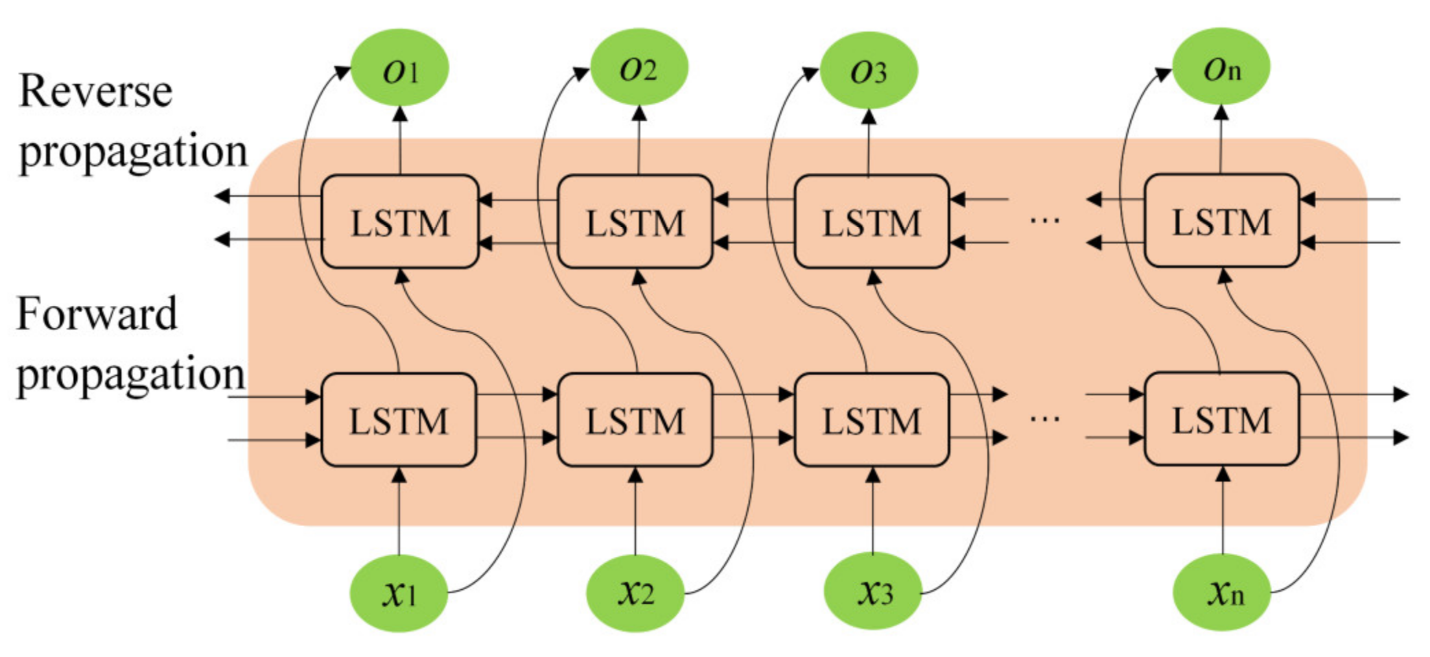
2.1. Bi-LSTM Model Structure

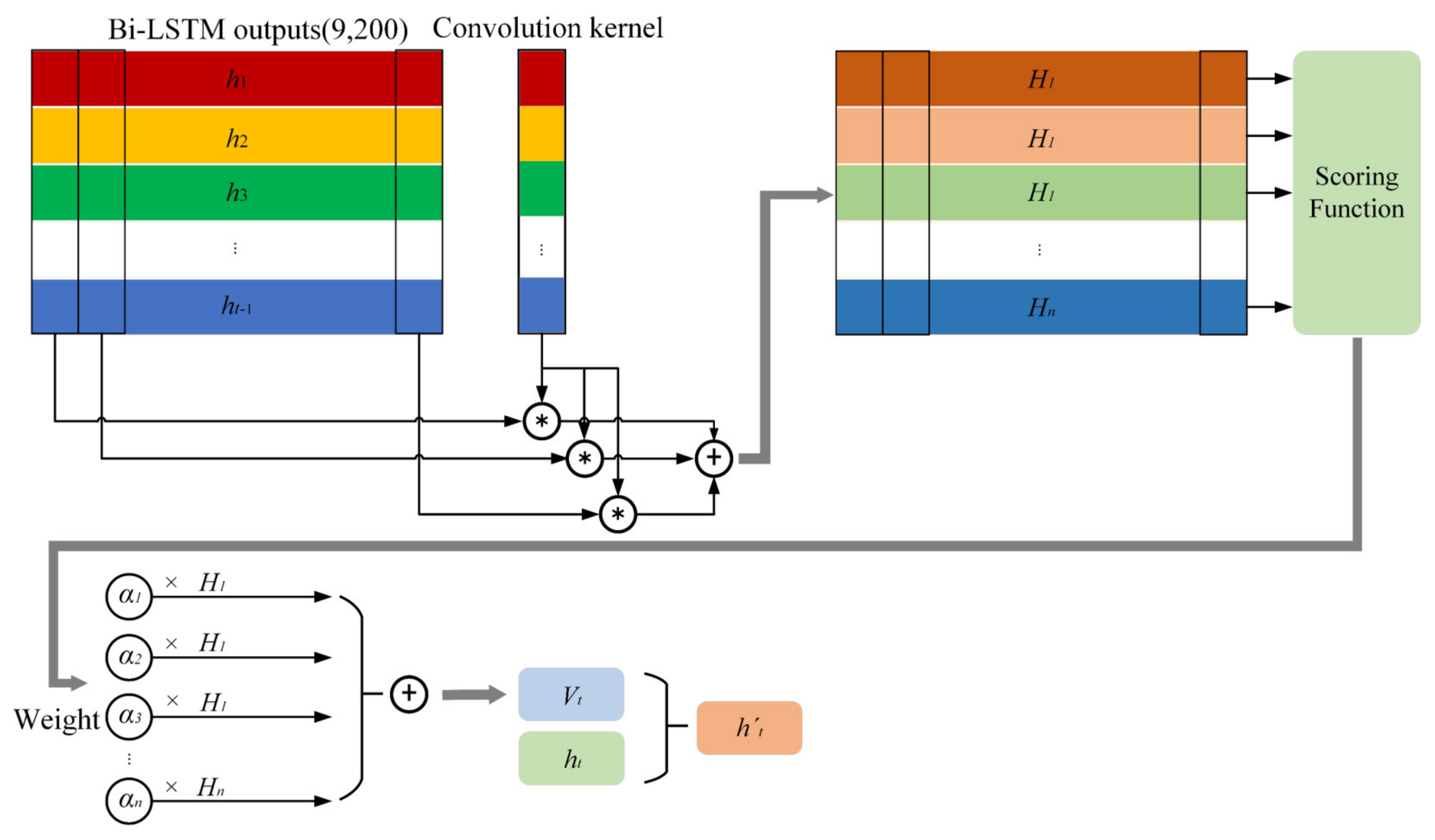
The LSTM network is known as long short-term memory network [30]. The concept of gating mechanism is proposed for the first time. Three gating mechanisms are used to effectively solve the problem of gradient disappearance and gradient explosion. The three control gates of LSTM are as follows: forgetting gate, input gate, and output gate, as shown in Figure 1.

In Figure 1, the black box represents the forgetting gate, the red box represents the input gate, and the green box represents the output gate. C_t−1 represents the long-term memory vector. h_t−1 represents the short-term memory vector (output vector). σ and tanh are activation function, and the activation function is used to add nonlinear factor to improve the expressive ability of neural networks. σ is generally sigmoid function. The principle of a gating mechanism is to generate control vectors (f_t, i_t, and O_t) with each element in the range of 0–1 through sigmoid function, and then use the control vectors to control the information to be forgotten, input, and output. The forgetting gate generates a vector f_t with each element in the range of 0–1, which controls the information to be forgotten. The input gate generates vector i_t control input information. The output gate generates vector O_t control output information. sigmoid and tanh are expressed in Equations (1) and (2):

$$sigmoid=\frac{1}{1+{\mathrm{e}}^{-z}}$$

(1)

$$tanh=\frac{{\mathrm{e}}^z-{\mathrm{e}}^{-z}}{{\mathrm{e}}^z+{\mathrm{e}}^{-z}}$$

(2)

where, z is the input variable.

The gating mechanism is expressed in Equations (3)–(5):

$$f_{\mathrm{t}}=\sigma \left(W_{xf}{X}_t+W_{hf}{h}_{t-1}+W_{cf}{C}_{t-1}+b_f\right)$$

(3)

$$i_t=\sigma \left(W_{xi}{X}_t+W_{hi}{h}_{t-1}+W_{ci}{C}_{t-1}+b_i\right)$$

(4)

$$O_t=\sigma \left(W_{xo}{X}_t+W_{ho}{h}_{t-1}+W_{co}{C}_{t-1}+b_o\right)$$

(5)

where i_t, O_t, and f_t are control vectors of input gate, output gate, and forgetting gate respectively. X_t is the input of sampling time t. W_xf, W_hf, W_cf, W_xi, W_hi, W_ci, W_xo, W_ho, and W_co are the corresponding weights.

Under the control of the input gate and the forgetting gate, LSTM can selectively use valid data, the updating formula of C_t and h_t (output vector) are defined as:

$$C_t=f_t{C}_{t-1}+i_{t}tanh\left(W_{xc}{X}_t+W_{hc}{h}_{t-1}+b_c\right)$$

(6)

$$h_t=O_t\times tanh\left(C_t\right)$$

(7)

where W_xc, W_hc are the corresponding weights, b_c is the bias.

Because single LSTM can not extract feature information from two directions. This paper uses Bi-LSTM [40,41], a variant of LSTM, to extract forward temporal feature and reverse temporal feature of historical data through forward propagation and reverse propagation respectively. For example, when the data of the tenth sampling time is predicted, the data of the first nine sampling times are used. The positive sequence method is used to transfer the nine sampling times to the forward propagation layer, and the reverse sequence method is used to send the data of the nine sampling times to the reverse propagation layer. Reverse propagation of data means that time series are transmitted to the model in reverse order, unlike BP algorithm, which uses the error generated by the output of the model to transmit to the input of the model through chain derivation rule. The specific structure of Bi-LSTM is shown in Figure 2.

In Figure 2, LSTM is the structure shown in Figure 1, X = [x₁, x₂, x₃,……x_t−1, x_t] means input data, x_i∈R^l×v (i = 1, 2, 3,…, t). l represents the length of the input time series, v represents the dimensions of the input variables. The output characteristic is represented by O = [o₁, o₂, o₃,…,o_t−1, o_t]. The first layer LSTM represents the forward propagation layer, the second layer LSTM represents the reverse propagation layer.

2.2. TPA Structure

TPA uses the output characteristics of Bi-LSTM to generate the weight α_i of each state through the scoring function. The corresponding row vector of convolution result is multiplied and accumulated to get the context vector V_t, and finally get the vector h_t and the prediction value y_t−1+Δ. TPA uses convolution kernel to extract the deep information contained in the state of single feature in the output features of Bi-LSTM at all sampling times, realizes temporal pattern extraction, as shown in Figure 3.

In Figure 3, different colors are used to represent temporal characteristics at different sampling times, H^C is the temporal pattern extracted by convolution. α_i (i = 1, 2, 3, …, n) is the weight generated by the scoring function, V_t is the weighted sum of α_i and H_i. The row vector of h = [h^T₁, h^T₂, h^T₃, …, h^T_t−1]∈R^n×t−1 represents the state of single feature at all sampling times, that is, the vector composed of the states of all sampling times of single feature. The column vector of h represents all the states of same sampling time; that is, a vector composed of all features at the same sampling time. A set of filters is used to extract the temporal information of single feature at different sampling times.

The detailed process of TPA can be expressed in Equations (8)–(10):

$$H_{i,j}^C={\displaystyle \sum _{l=1}^w{h}_{i,\left(t-w-1+l\right)}\times C_{j,T-w+l}}$$

(8)

where C_i∈R^1×T is the convolution kernel; w is the prediction window; T is the maximum attention length of the model; assume T = w. H^C∈R^n×k is the convolution result; i represents i-th (i = 1, 2, 3, …, n) row vector of h; j represents the j-th (j = 1, 2, 3, …, k) convolution kernel; there are a total of k convolution kernels; $H_{i,j}^C$ is the convolution value of the i-th row vector and the j-th convolution kernel.

$$f\left(H_i,h_t\right)=H_i{W}_a{h}_t$$

(9)

where $H_i$ is the i-th row of H^C, W_α∈R^k×m. Attention weight α_i can be obtained from (10):

$$a_i=sigmoid\left(f\left(H_i,h_t\right)\right)$$

(10)

where h_t∈R^m, f is scoring function, α_i (i = 1, 2, 3, …, n) is attention weight.

3. Ship Roll Angle Prediction Algorithm Based on Bi-LSTM-TPA Model

At present, the prediction of ship roll angle only considers the case of single input. Whether other motion attitude data and marine environment data, such as relative wind speed, relative wind direction, ship roll angle acceleration, pitch angle, rudder angle, and other information are beneficial to prediction can only be judged by prior knowledge. If the network can focus on the most favorable features for prediction, and study the relationship between the features, the accuracy of prediction will be improved. Attention mechanism can calculate the weight of each dimensional input feature. If the weight is large, it means that the feature is more favorable for prediction. If the weight is small, it means that the feature has less contribution to ship roll angle prediction.

Bi-LSTM extracts temporal features of multidimensional time series from forward and reverse directions. TPA is located in the back of the Bi-LSTM, which takes the output features of Bi-LSTM network as the input, extracts the deep information contained in the state of single feature at all sampling times, and focus on temporal patterns that are good for forecasting. Combining the two models can take full advantage of each model and improve the prediction accuracy. The prediction process of the ship roll angle prediction algorithm based on the Bi-LSTM-TPA model is shown in Figure 4.

Figure 4 shows the ship roll angle prediction process of the Bi-LSTM-TPA model. The input data of the model includes ship roll angle, relative wind speed, relative wind direction, roll acceleration, trim, and rudder angle. The output data of the model is ship roll angle. Firstly, the historical data such as ship roll angle, relative wind speed, relative wind direction, etc. are preprocessed, including data cleaning, data interpolation, denoising and increasing the weight of ship roll angle data. The preprocessed data is input into Bi-LSTM network, and Bi-LSTM model extracts temporal features h from forward and reverse directions. After that, the temporal pattern H^C of cross time feature is extracted by convolution layer. The convolution kernel of convolution layer is set as a group every ten sampling times. The first nine sampling times are used for model training, the tenth sampling time is used for model prediction. The dimension of the input variable is 6.

The attention weight α_i of each row vector in H^C is calculated by scoring function and sigmoid function, α_i represents the contribution of the i-th feature to the prediction task. Therefore, TPA can only focus on some dimensions of deep feature H^C. Finally, the predicted value y_t−1+Δ is obtained by Equations (11)–(13) and the model is evaluated by the evaluation index.

$$V_t={\displaystyle \sum _{i=l}^n{\alpha }_i{H}_i}$$

(11)

where, V_t∈R^k, α_i (i = 1, 2, 3,…, n) is attention weight, V_t is context vector. The vector is obtained and the predicted value y_t−1+Δ is generated:

$$h_t^{\prime }=W_h{h}_t+W_v{v}_t$$

(12)

$$y_{t-1+\Delta }=W_{h^{\prime }}{h}_t^{\prime }$$

(13)

where, $h_t^{\prime }$∈R^m, W_h∈R^m×m, W_v∈R^m×k, W_h′∈R^n×m, y_t−1+Δ∈Rⁿ.

4. Simulation Results of Roll Angle Prediction

In order to prove the effectiveness of the proposed method, using the real ship motion data obtained when ships sail on sea as the dataset. The main ship motion includes ship roll angle, ship roll acceleration, rudder angle, relative wind speed and wind direction etc., with a total of 32,371 data points. The first 80% of all data is used as training dataset, and the last 20% as test dataset.

4.1. Evaluation Indicators

Compare the Bi-LSTM-TPA prediction model with single LSTM model and SVM model, mean square error (MSE), mean absolute percentage error (MAPE), mean absolute error (MAE), promotion mean square error (PMSE), promotion mean absolute percentage error (PMAPE), and promotion mean absolute error (PMAE) are used as evaluation indicators. Among them, MSE reflects the difference between the real value and the predicted value, MAPE represents the average deviation of the predicted value from the real value. Because the magnitude of the value in the dataset is very small, if MSE is used as the loss function, the loss function will be close to 0, but the prediction effect is very poor. Therefore, MAPE is used as the loss function. MAE is the average value of the absolute value of the error between the predicted value and the real value. The average absolute error can avoid the problem of mutual cancellation of errors, so it can accurately reflect the actual prediction error. Three kinds of promotion percentage error can reflect the difference of the two models in the same error index. MSE, MAPE, MAE, PMSE, PMAPE, and PMAE are shown in Equations (14)–(19):

$$\mathrm{MSE}=\frac{\left({\displaystyle {\sum }_{i=1}^N|y\left(i\right)-\hat{y}\left(i\right){|}^2}\right)}{N}$$

(14)

$$\mathrm{MAPE}=\frac{\left({\displaystyle {\sum }_{i=1}^N|y\left(i\right)-\hat{y}\left(i\right)/y\left(i\right)|}\right)}{N}$$

(15)

$$\mathrm{MAE}=\frac{\left({\displaystyle {\sum }_{i=1}^N|y\left(i\right)-\hat{y}\left(i\right)|}\right)}{N}$$

(16)

$$\mathrm{PMSE}=\frac{{\mathrm{MSE}}_1-{\mathrm{MSE}}_2}{{\mathrm{MSE}}_1}$$

(17)

$$\mathrm{PMAPE}=\frac{{\mathrm{MAPE}}_1-{\mathrm{MAPE}}_2}{{\mathrm{MAPE}}_1}$$

(18)

$$\mathrm{PMAE}=\frac{{\mathrm{MAE}}_1-{\mathrm{MAE}}_2}{{\mathrm{MAE}}_1}$$

(19)

where, $y\left(i\right)$ is the real value, $\hat{y}\left(i\right)$ is the predicted value, N is the total number of sample points.

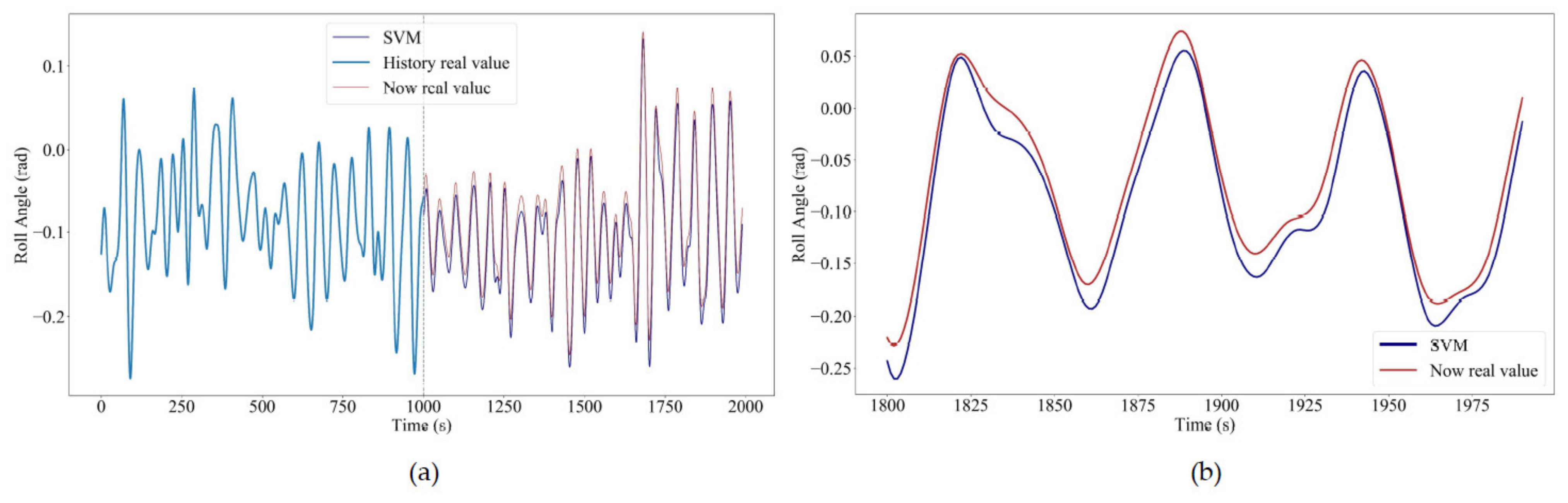
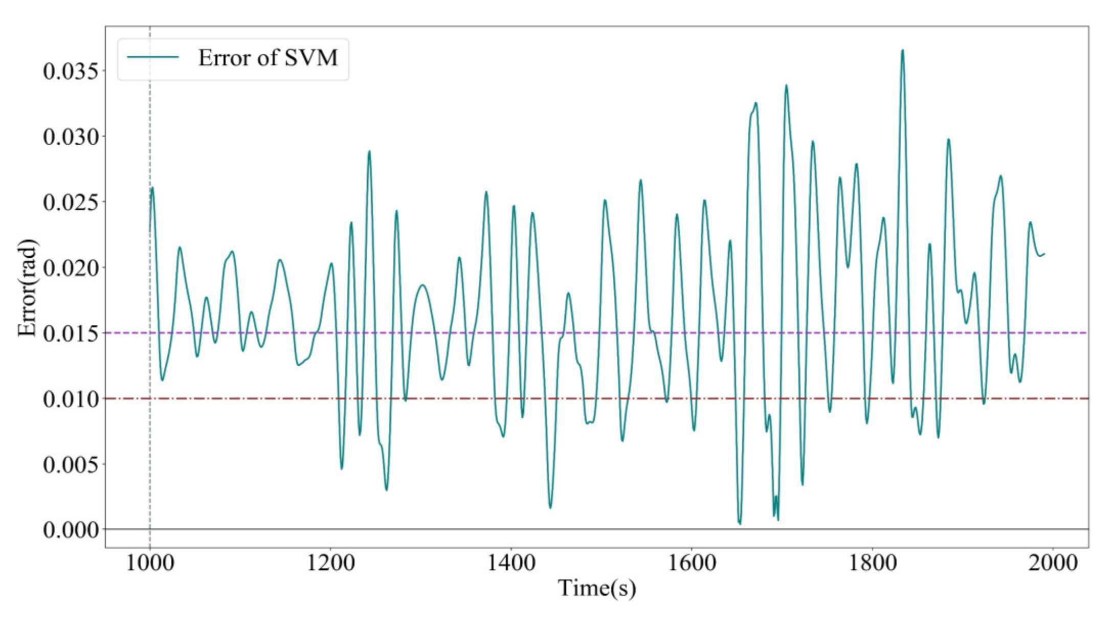
4.2. Prediction of Ship Roll Angle Based on SVM Model

In this paper, radial basis function (RBF) is used to map the input features to a high-dimensional feature space, in which the optimal classification hyperplane is constructed. The penalty parameter C of the error term is set to 10 and the nuclear coefficient γ is set to 1. The prediction window is set to 10, which is consistent with the prediction windows of Bi-LSTM-TPA model and LSTM model. The results of prediction of ship roll angle using SVM model are shown in Figure 5.

Figure 5a shows the ship roll angle prediction results of SVM model, showing the change of ship roll angle within 2000 s. The blue solid line represents the historical data, the data after 1000 s is the prediction data, the purple solid line represents the SVM prediction data, the red solid line represents the real data. Figure 5b shows the prediction results of ship roll angle based on SVM model in 1800 s–2000 s. It can be seen from Figure 5b that the deviation of the SVM prediction curve from the real data curve is serious, especially when the direction of ship roll angle changes, the prediction curve can not track the real ship roll angle curve in time, causes a large error near the extremum of the real ship roll angle curve. However, the overall trend of SVM prediction curve is basically consistent with the real data curve.

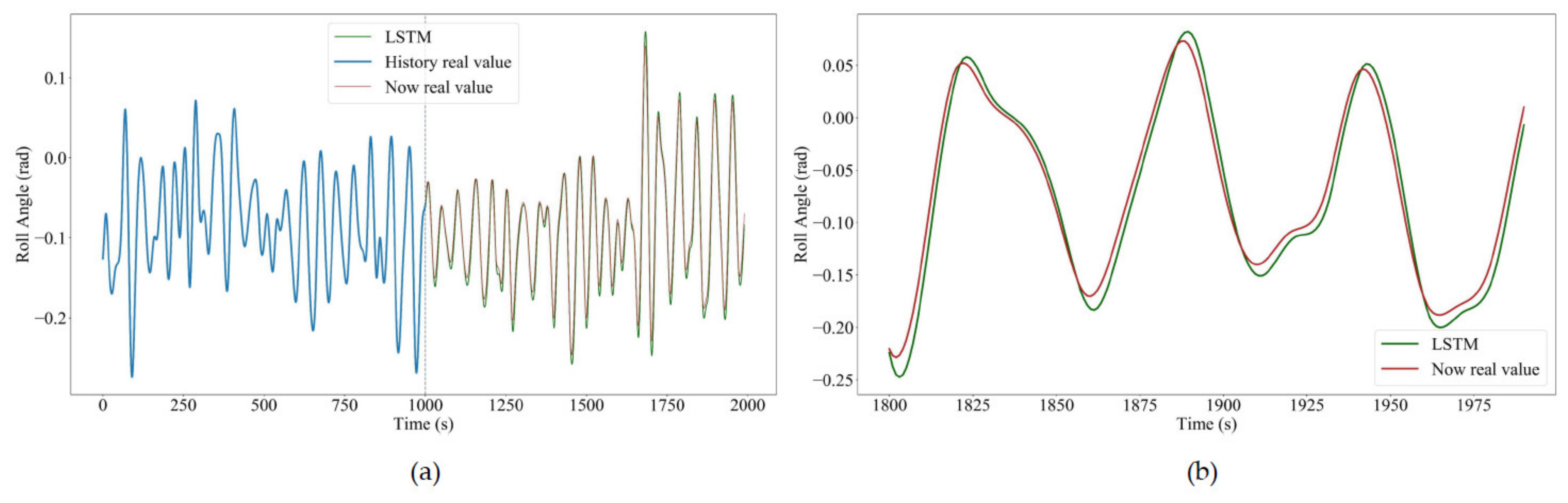
4.3. Prediction of Ship Roll Angle Based on LSTM Model

In order to compare Bi-LSTM-TPA model, three LSTM layers are used. The dimension of state vector of each layer is 100, the number of iterations is 60, the batch size is 64. In order to prevent over-fitting, dropout layer is added between each layer, the parameter is set to 0.2, the prediction window is 10. Single LSTM model is used to predict the ship roll angle of a ship, the results are shown in Figure 6.

Figure 6a shows the ship roll angle prediction results of LSTM model, showing the change of ship roll angle in 2000 s. The blue solid line is the historical data, the data after 1000 s is the prediction data, the green solid line is the LSTM prediction data, the red solid line is the real data. Figure 6b shows the prediction results of the LSTM model in 1800 s–2000 s. It can be seen from Figure 6b that the LSTM prediction curve tracks the real ship roll angle curve well. When the real ship roll angle curve is near the extreme value, the LSTM model can not fully capture the changes of the real ship roll angle data, but the prediction results near the extreme value is better than the SVM model. In the region where the real ship roll angle curve is in a consistent rise or a consistent fall, such as 1860 s–1880 s, the LSTM prediction curve has a good tracking effect on the real ship roll angle curve, the overall change trend of LSTM prediction curve is basically consistent with the real ship roll angle curve.

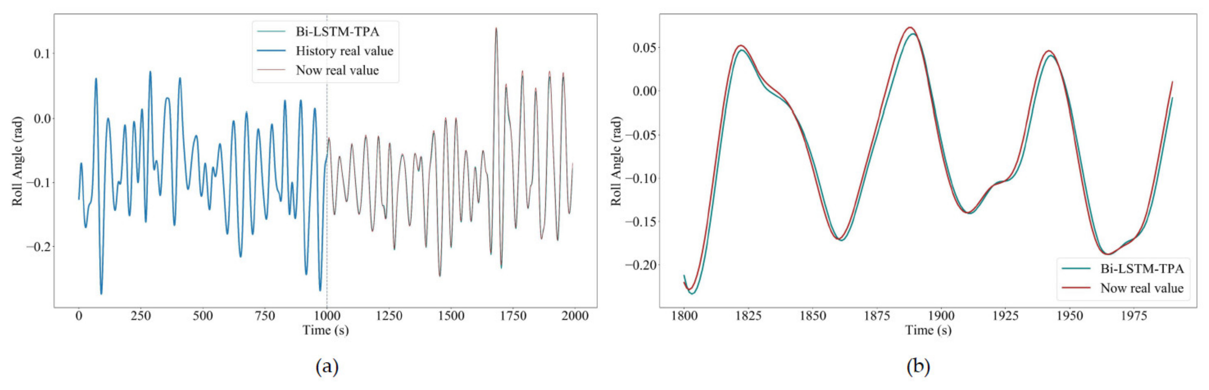
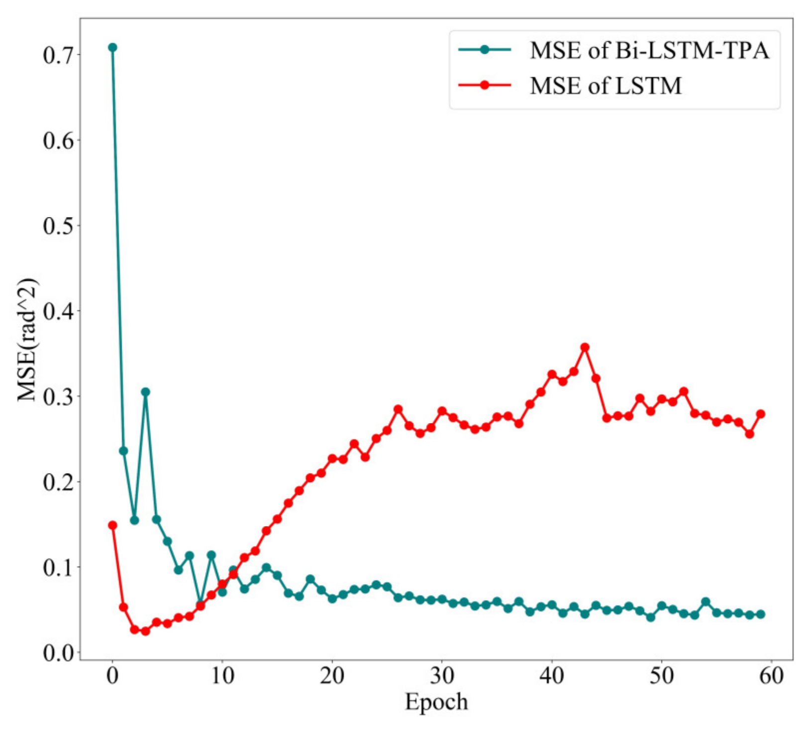
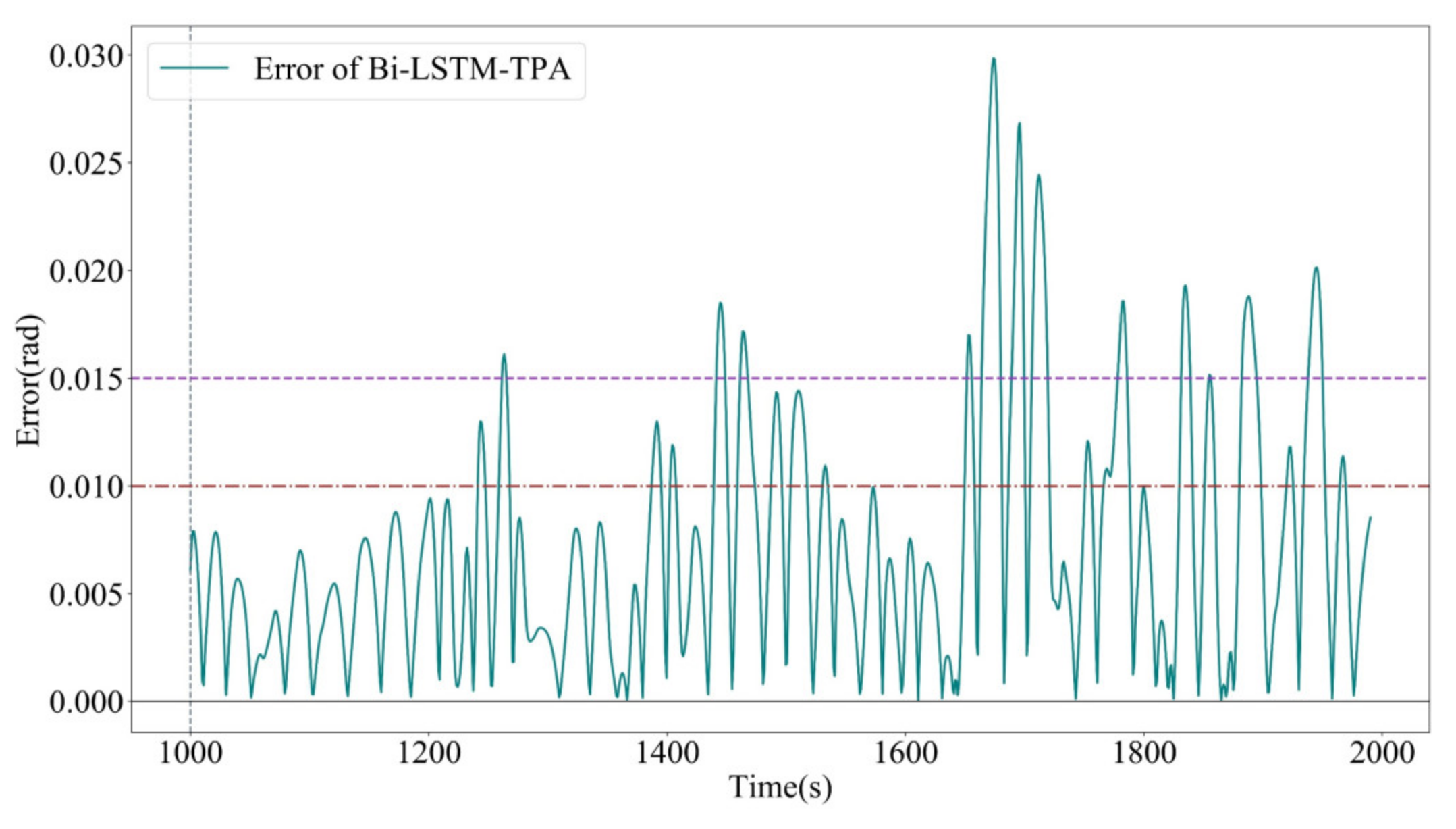
4.4. Prediction of Ship Roll Angle Based on Bi-LSTM-TPA

In the construction of the model, using three Bi-LSTM layers. The dimensions of the state vectors of the forward layer and the reverse layer of each layer are 100. A prediction is generated for every ten numbers. The number of iterations is 60 and the batch size is 64. In order to prevent over fitting, dropout layer is added between each layer, and the parameter is set to 0.2. Bi-LSTM-TPA is used to predict the ship roll angle, and the prediction results are shown in Figure 7.

Figure 7a shows the ship roll angle prediction results of Bi-LSTM-TPA model, showing the change of ship roll angle within 2000 s. The blue solid line represents the historical data, the data after 1000 s is the prediction data, the green solid line represents the Bi-LSTM-TPA prediction data curve, and the red solid line represents the real ship roll angle curve. Figure 7b shows the ship roll prediction results of Bi-LSTM-TPA model in 1800 s–2000 s, it can be seen from Figure 7b that the Bi-LSTM-TPA prediction curve well fits the real ship roll angle curve. When the direction of heel changes, Bi-LSTM-TPA model can capture the change of real ship roll angle data, and the prediction results near the extreme point are significantly better than those of SVM and LSTM model. Even in 1900 s–1925 s, it can track the change of ship roll angle perfectly. The Bi-LSTM-TPA prediction curve has a good tracking effect on the real ship roll angle curve when the ship roll angle curve is in the region of consistent rise or consistent decline, such as 1860 s–1880 s.

In order to show more clearly that the Bi-LSTM-TPA model is better than the single LSTM model, Figure 8 and Figure 9 show the error of the two models under the condition of Epoch = 60.

Figure 8 shows the attenuation of MAPE of the two models. The MAPE of single LSTM model changes greatly, the MAPE curve of LSTM model is compared with that of Bi-LSTM-TPA model, the MAPE curve of Bi-LSTM-TPA model is basically below the error curve of LSTM model, which indicates that the MAPE index of Bi-LSTM-TPA model performs best in each training period.

Figure 9 shows the MSE attenuation of the two models at Epoch = 60. The MSE curve of Bi-LSTM-TPA model shows a downward trend in the whole process of model training, whereas the MSE curve of single LSTM shows a situation that the error curve decreases at the beginning of the training process and then increases, finally stabilizes at about 0.25. Before Epoch = 10, single LSTM model performs better in MSE index. After Epoch = 10, the MSE index of Bi-LSTM-TPA model performs better.

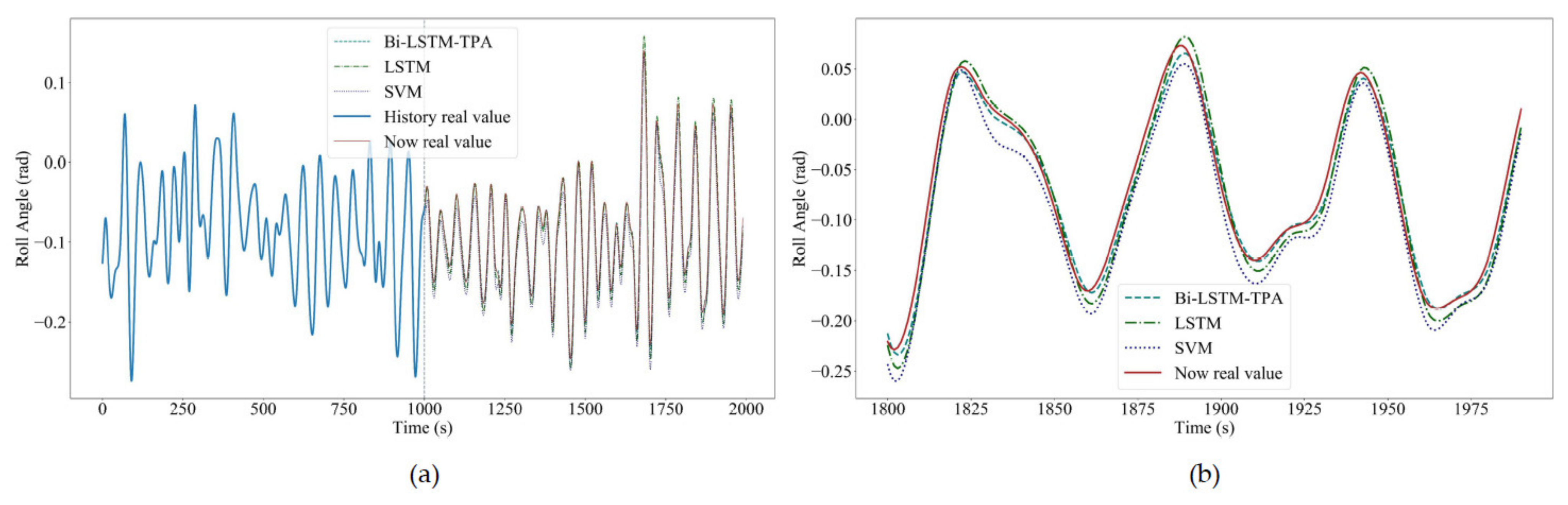
4.5. Comparison of Prediction Results of Three Models

In order to better compare the prediction performance of the three different models (Bi-LSTM, LSTM, SVM) on ship roll angle, the prediction results of the three models on the real ship dataset are shown in Figure 10.

Figure 10a shows the ship roll angle prediction results of three different models, showing the change of ship roll angle within 2000 s. The blue solid line represents the historical data, and the data after 1000 s is the prediction data. Figure 10a intuitively shows the prediction effect of the three models, Bi-LSTM-TPA model has the best prediction effect. Figure 10b shows the ship roll angle prediction results of the three models in 1800 s–1975 s. Near the extreme point, Bi-LSTM-TPA has the best prediction effect and the strongest tracking ability. In the region where the ship roll angle curve is in a consistent rise or a consistent decline, the prediction results of all models are improved, but Bi-LSTM-TPA has the best prediction effect. To sum up, Bi-LSTM-TPA model is the best in both the extreme point and the area of consistent rise or decline. In order to show the deviation between the predicted ship roll angle value and the true ship roll angle value after 1000 s in detail, Figure 11, Figure 12 and Figure 13 shows the absolute deviation between the predicted ship roll angle value and the true ship roll angle value of the three models in 1000 s–2000 s, that is Error = |y_pre − y_real|.

In Figure 11, the red dotted line indicates Error = 0.010 (rad) and the purple dotted line indicates Error = 0.015 (rad). As can be seen from Figure 11, Error curve is mainly above Error = 0.010 (rad). The maximum value of Error curve appeared around 1830 s, and the maximum value is 0.037 (rad).

In Figure 12, the red dotted line indicates Error = 0.010 (rad) and the purple dotted line indicates Error = 0.015 (rad). As can be seen from the Figure 12, Error curve is mainly below Error = 0.015 (rad). The maximum value of Error curve appears around 1700 s, and the maximum value is 0.036 (rad).

In Figure 13, the red dotted line indicates Error = 0.010 (rad) and the purple dotted line indicates Error = 0.015 (rad), the gray dashed line indicates the prediction line at 1000 s. As can be seen from the Figure 13, Error curve is mainly below Error = 0.010 (rad). The maximum value of Error curve appears around 1650 s, and the maximum value is 0.030 (rad). If Error = 0.010 (rad) and Error = 0.015 (rad) are used as boundary value, the Error curve of SVM model is mainly in the range of 0.010 (rad) < Error < 0.025 (rad), the Error curve of LSTM model is mainly in the range of 0 (rad) < Error < 0.015 (rad), and the Error curve of Bi-LSTM-TPA model is mainly in the range of 0 (rad) < Error < 0.010 (rad).

Table 1. Comparison of error index of three models.

	Bi-LSTM-TPA	LSTM	SVM
MSE	8.01 × 10−5	1.48 × 10−4	3.26 × 10−4
MAPE (%)	12.0	16.0	27.9
MAE	0.007	0.010	0.017

shows the prediction Error index of the three prediction models.

In Table 1, the MSE, MAPE, and MAE of Bi-LSTM-TPA model are 8.01 × 10⁻⁵,12.0% and 0.007 respectively. The MSE of single LSTM model is 1.48 × 10⁻⁴, which is lower than MSE = 3.26 × 10⁻⁴ of SVM. The MAPE and MAE of LSTM are 16.0% and 0.010 respectively, and those of SVM are 27.9% and 0.017 respectively. Compared with the three error indexes, Bi-LSTM-TPA model has the best prediction performance. In order to show the performance improvement degree of Bi-LSTM-TPA model compared with LSTM and SVM models in three error indicators,

Table 2. Promotion percentage index of Bi-LSTM-TPA.

	SVM	LSTM
PMSE (%)	75.4	45.8
PMAPE (%)	56.6	25.0
PMAE (%)	58.8	30.0

shows the promotion percentage error indicators of Bi-LSTM-TPA model.

In Table 2, compared with LSTM model, MSE index of Bi-LSTM-TPA model decreased by 45.8%, MAPE index decreased by 25.0%, MAE index decreased by 30.0%. Compared with SVM model, the MSE index of Bi-LSTM-TPA model decreased by 75.4%, the MAPE index decreased by 56.6%, and the MAE index decreased by 58.8%. Bi-LSTM-TPA model has the best performance in MSE, MAPE, and MAE, since Bi-LSTM can extract temporal features from forward and reverse, and TPA can focus on extracting deep features beneficial for prediction.

The prediction data and statistical results of real ship data show that the Bi-LSTM-TPA combination model has excellent prediction performance; the prediction effect is more accurate, stable, and reliable than the other two models. It can better predict the change of ship roll angle when ships sail on the sea, so as to provide control basis for controlling the ship into a safe state in advance and ensure the safety of the ship during navigation security.

5. Conclusions

In view of the nonlinear and high randomness of the ship motion attitude when ships sail on the sea, a combined model of ship roll angle prediction based on Bi-LSTM and TPA is proposed. The Bi-LSTM-TPA model combines the advantages of Bi-LSTM and TPA model. It can not only extract the time feature of ship roll angle data from two directions, but also focus on the depth feature which is more beneficial for prediction. It solves the problem that the existing single neural network model and traditional machine learning methods are difficult to make accurate prediction of the real ship roll angle. In order to objectively compare the effectiveness of the algorithm, 80% of the real ship data samples are used as the training set and 20% as the test set. Results show that the Bi-LSTM-TPA model has better prediction accuracy than SVM and LSTM algorithm. In the case of mastering the historical ship’s motion posture, it can predict the change of a ship’s motion posture in a short time in the future, so as to improve the safety and stability of ship’s water operation, which has important application value.

References

1. Yu, L.; Ma, N.; Wang, S. Parametric Roll Prediction of the KCS Containership in Head Waves with Emphasis on the Roll Damping and Nonlinear Restoring Moment. Ocean Eng. 2019, 188, 106298. [Google Scholar] [CrossRef]
2. Li, Y.; He, Y.; Su, Y. Forecasting the daily power output of a grid-connected photovoltaic system based on multivariate adaptive regression splines. Appl. Energy 2016, 180, 392–401. [Google Scholar] [CrossRef]
3. Huang, S.J.; Huang, C.L. Control of an Inverted Pendulum Using Grey Prediction Model. IEEE Trans. Ind. Appl. 2000, 36, 452–458. [Google Scholar] [CrossRef]
4. Yazdanbakhsh, O.; Dick, S. Forecasting of Multivariate Time Series via Complex Fuzzy Logic. IEEE Trans. Syst. Man Cybern. Syst. 2017, 47, 2160–2171. [Google Scholar] [CrossRef]
5. Cai, M.; Pipattanasomporn, M.; Rahman, S. Day-ahead building-level load forecastsusing deep learning vs. traditional time-series techniques. Appl. Energy 2019, 236, 1078–1088. [Google Scholar] [CrossRef]
6. Gonzalez, J.P.; Roque, A.M.S.; Perez, E.A. Forecasting Functional Time Series with a New Hilbertian ARMAX Model: Application to Electricity Price Forecasting. IEEE Trans. Power Syst. 2018, 33, 545–556. [Google Scholar] [CrossRef]
7. De Lima Silva, P.C.; Sadaei, H.J.; Ballini, R.; Guimaraes, F.G. Probabilistic Forecasting with Fuzzy Time Series. IEEE Trans. Fuzzy Syst. 2020, 28, 1771–1784. [Google Scholar] [CrossRef]
8. Li, R.; Jiang, C.; Zhu, F.; Chen, X. Traffic Flow Data Forecasting Based on Interval Type-2 Fuzzy Sets Theory. IEEE CAA J. Autom. Sin. 2016, 3, 141–148. [Google Scholar] [CrossRef]
9. Jiang, H.; Duan, S.; Huang, L.; Han, Y.; Yang, H.; Ma, Q. Scale Effects in AR Model Real-Time Ship Motion Prediction. Ocean Eng. 2020, 203, 107202. [Google Scholar] [CrossRef]
10. Li, R.; Huang, Y.; Wang, J. Long-Term Traffic Volume Prediction Based on K-Means Gaussian Interval Type-2 Fuzzy Sets. IEEE CAA J. Autom. Sin. 2019, 6, 1344–1351. [Google Scholar] [CrossRef]
11. Liu, B.; Nowotarski, J.; Hong, T.; Weron, R. Probabilistic Load Forecasting via Quantile Regression Averaging on Sister Forecasts. IEEE Trans. Smart Grid 2015, 8, 730–737. [Google Scholar] [CrossRef]
12. Benetazzo, A.; Barbariol, F.; Bergamasco, F.; Torsello, A.; Carniel, S.; Sclavo, M. Stereo Wave Imaging from Moving Vessels: Practical Use and Applications. Coast. Eng. 2016, 109, 114–127. [Google Scholar] [CrossRef]
13. Bergamasco, F.; Benetazzo, A.; Barbariol, F.; Carniel, S.; Sclavo, M. Multi-View Horizon-Driven Sea Plane Estimation for Stereo Wave Imaging on Moving Vessels. Comput. Geosci. 2016, 95, 105–117. [Google Scholar] [CrossRef] [Green Version]
14. Wu, J.; Liu, H.; Wei, G.; Song, T.; Zhang, C.; Zhou, H. Flash Flood Forecasting Using Support Vector Regression Model in a Small Mountainous Catchment. Water 2019, 11, 1327. [Google Scholar] [CrossRef] [Green Version]
15. Jiang, H.; Zhang, Y.; Muljadi, E.; Zhang, J.J.; Gao, D.W. A Short-Term and High-Resolution Distribution System Load Forecasting Approach Using Support Vector Regression with Hybrid Parameters Optimization. IEEE Trans. Smart Grid. 2018, 9, 3341–3350. [Google Scholar] [CrossRef]
16. Liu, Q.; Shen, Y.; Wu, L.; Li, J.; Zhuang, L.; Wang, S. A Hybrid FCW-EMD and KF-BA-SVM Based Model for Short-Term Load Forecasting. CSEE JPES 2018, 4, 226–237. [Google Scholar] [CrossRef]
17. Wang, X. Ladle Furnace Temperature Prediction Model Based on Large-Scale Data with Random Forest. IEEE CAA J. Autom. Sin. 2017, 4, 770–774. [Google Scholar] [CrossRef]
18. Zhang, W.; Zhang, H.; Liu, J.; Li, K.; Yang, D.; Tian, H. Weather Prediction with Multiclass Support Vector Machines in the Fault Detection of Photovoltaic System. IEEE CAA J. Autom. Sin. 2017, 4, 520–525. [Google Scholar] [CrossRef]
19. Yin, J.-C.; Perakis, A.N.; Wang, N. A Real-Time Ship Roll Motion Prediction Using Wavelet Transform and Variable RBF Network. Ocean Eng. 2018, 160, 10–19. [Google Scholar] [CrossRef]
20. Mulia, I.E.; Asano, T.; Nagayama, A. Real-Time Forecasting of near-Field Tsunami Waveforms at Coastal Areas Using a Regularized Extreme Learning Machine. Coast. Eng. 2016, 109, 1–8. [Google Scholar] [CrossRef]
21. Li, C.; Wang, L.; Zhang, G.; Wang, H.; Shang, F. Functional-Type Single-Input-Rule-Modules Connected Neural Fuzzy System for Wind Speed Prediction. IEEE CAA J. Autom. Sin. 2017, 4, 751–762. [Google Scholar] [CrossRef]
22. Rafiei, M.; Niknam, T.; Aghaei, J.; Shafie-Khah, M.; Catalao, J.P.S. Probabilistic Load Forecasting Using an Improved Wavelet Neural Network Trained by Generalized Extreme Learning Machine. IEEE Trans. Smart Grid 2018, 9, 6961–6971. [Google Scholar] [CrossRef]
23. Zhang, P.; Jia, Y.; Gao, J.; Song, W.; Leung, H. Short-Term Rainfall Forecasting Using Multi-Layer Perceptron. IEEE Trans. Big Data 2020, 6, 93–106. [Google Scholar] [CrossRef]
24. Gong, X.; Cardenas-Barrera, J.L.; Castillo-Guerra, E.; Cao, B.; Saleh, S.A.; Chang, L. Bottom-Up Load Forecasting with Markov-Based Error Reduction Method for Aggregated Domestic Electric Water Heaters. IEEE Trans. Ind. Appl. 2019, 55, 6401–6413. [Google Scholar] [CrossRef]
25. Zhang, C.-Y.; Chen, C.L.P.; Gan, M.; Chen, L. Predictive Deep Boltzmann Machine for Multiperiod Wind Speed Forecasting. IEEE Trans. Sustain. Energy 2015, 6, 1416–1425. [Google Scholar] [CrossRef]
26. Hinton, G.E.; Osindero, S.; Teh, Y.-W. A Fast Learning Algorithm for Deep Belief Nets. Neural Comput. 2006, 18, 1527–1554. [Google Scholar] [CrossRef]
27. Ouyang, T.; He, Y.; Li, H.; Sun, Z.; Baek, S. Modeling and Forecasting Short-Term Power Load With Copula Model and Deep Belief Network. IEEE Trans. Emerg. Top. Comput. Intell. 2019, 3, 127–136. [Google Scholar] [CrossRef] [Green Version]
28. Barra, S.; Carta, S.M.; Corriga, A.; Podda, A.S.; Recupero, D.R. Deep Learning and Time Series-to-Image Encoding for Financial Forecasting. IEEE CAA J. Autom. Sin. 2020, 7, 683–692. [Google Scholar] [CrossRef]
29. Tang, X.; Dai, Y.; Liu, Q.; Dang, X.; Xu, J. Application of Bidirectional Recurrent Neural Network Combined with Deep Belief Network in Short-Term Load Forecasting. IEEE Access 2019, 7, 160660–160670. [Google Scholar] [CrossRef]
30. Hochreiter, S.; Schmidhuber, J. Long short-term memory. Neural Comput. 1997, 9, 1735–1780. [Google Scholar] [CrossRef]
31. Liang, R.; Kong, F.; Xie, Y.; Tang, G.; Cheng, J. Real-Time Speech Enhancement Algorithm Based on Attention LSTM. IEEE Access 2020, 8, 48464–48476. [Google Scholar] [CrossRef]
32. Poornima, S.; Pushpalatha, M. Prediction of Rainfall Using Intensified LSTM Based Recurrent Neural Network with Weighted Linear Units. Atmosphere 2019, 10, 668. [Google Scholar] [CrossRef] [Green Version]
33. Zhao, X.; Chen, Y.; Guo, J.; Zhao, D. A Spatial-Temporal Attention Model for Human Trajectory Prediction. IEEE CAA J. Autom. Sin. 2020, 7, 965–974. [Google Scholar] [CrossRef]
34. Tan, M.; Yuan, S.; Li, S.; Su, Y.; Li, H.; He, F.H. Ultra-Short-Term Industrial Power Demand Forecasting Using LSTM Based Hybrid Ensemble Learning. IEEE Trans. Power Syst. 2020, 35, 2937–2948. [Google Scholar] [CrossRef]
35. Mutavhatsindi, T.; Sigauke, C.; Mbuvha, R. Forecasting Hourly Global Horizontal Solar Irradiance in South Africa Using Machine Learning Models. IEEE Access 2020, 8, 198872–198885. [Google Scholar] [CrossRef]
36. Wang, K.; Qi, X.; Liu, H. Photovoltaic Power Forecasting Based LSTM-Convolutional Network. Energy 2019, 189, 116225. [Google Scholar] [CrossRef]
37. Wang, K.; Qi, X.; Liu, H. A Comparison of Day-Ahead Photovoltaic Power Forecasting Models Based on Deep Learning Neural Network. Appl. Energy 2019, 251, 113315. [Google Scholar] [CrossRef]
38. Sun, Z.; Zhao, M. Short-Term Wind Power Forecasting Based on VMD Decomposition, ConvLSTM Networks and Error Analysis. IEEE Access 2020, 8, 134422–134434. [Google Scholar] [CrossRef]
39. Alhussein, M.; Aurangzeb, K.; Haider, S.I. Hybrid CNN-LSTM Model for Short-Term Individual Household Load Forecasting. IEEE Access 2020, 8, 180544–180557. [Google Scholar] [CrossRef]
40. Zhang, G.; Tan, F.; Wu, Y. Ship Motion Attitude Prediction Based on an Adaptive Dynamic Particle Swarm Optimization Algorithm and Bidirectional LSTM Neural Network. IEEE Access 2020, 8, 90087–90098. [Google Scholar] [CrossRef]
41. Saeed, A.; Li, C.; Danish, M.; Rubaiee, S.; Tang, G.; Gan, Z.; Ahmed, A. Hybrid Bidirectional LSTM Model for Short-Term Wind Speed Interval Prediction. IEEE Access 2020, 8, 182283–182294. [Google Scholar] [CrossRef]
42. Shih, S.Y.; Sun, F.K.; Lee, H.Y. Temporal Pattern Attention for Multivariate Time Series Forecasting. Mach. Learn. 2019, 108, 1421–1441. [Google Scholar] [CrossRef] [Green Version]
Figure 1. LSTM structure.
Jmse 09 00387 g001
Figure 2. Bi-LSTM structure.
Jmse 09 00387 g002
Figure 3. Schematic diagram of attention mechanism of TPA.
Jmse 09 00387 g003
Figure 4. Prediction process of Bi LSTM TPA model.
Jmse 09 00387 g004
Figure 5. Prediction results of ship roll angle based on SVM. (a) Ship roll angle prediction results of SVM model in 1000 s–2000 s; (b) Ship roll angle prediction results of SVM model based on local data (1800 s–2000 s).
Jmse 09 00387 g005
Figure 6. Ship roll angle prediction results of LSTM model. (a) Ship roll angle prediction results of LSTM model in 1000 s–2000 s; (b) Ship roll angle prediction results of LSTM model based on local data (1800 s 2000 s).
Jmse 09 00387 g006
Figure 7. Ship roll angle prediction results of Bi-LSTM-TPA model. (a) Ship roll angle prediction results of Bi LSTM TPA model in 1000 s–2000 s; (b) Ship roll angle prediction results of Bi LSTM TPA model based on local data (1800 s–2000 s).
Jmse 09 00387 g007
Figure 8. The change of MAPE in two models.
Jmse 09 00387 g008
Figure 9. The change of MSE of two models under the condition.
Jmse 09 00387 g009
Figure 10. Comparison of three different models for prediction of ship roll angle. (a) Ship roll angle prediction results of three different models in 1000 s–2000 s; (b) Ship roll angle prediction results of three models based on local data (1800 s–2000 s).
Jmse 09 00387 g010
Figure 11. The absolute value of the deviation between the predicted value of SVM and the true value.
Jmse 09 00387 g011
Figure 12. The absolute value of the deviation between the predicted value of LSTM and the true value.
Jmse 09 00387 g012
Figure 13. The absolute value of deviation between predicted and true value of Bi-LSTM-TPA.
Jmse 09 00387 g013