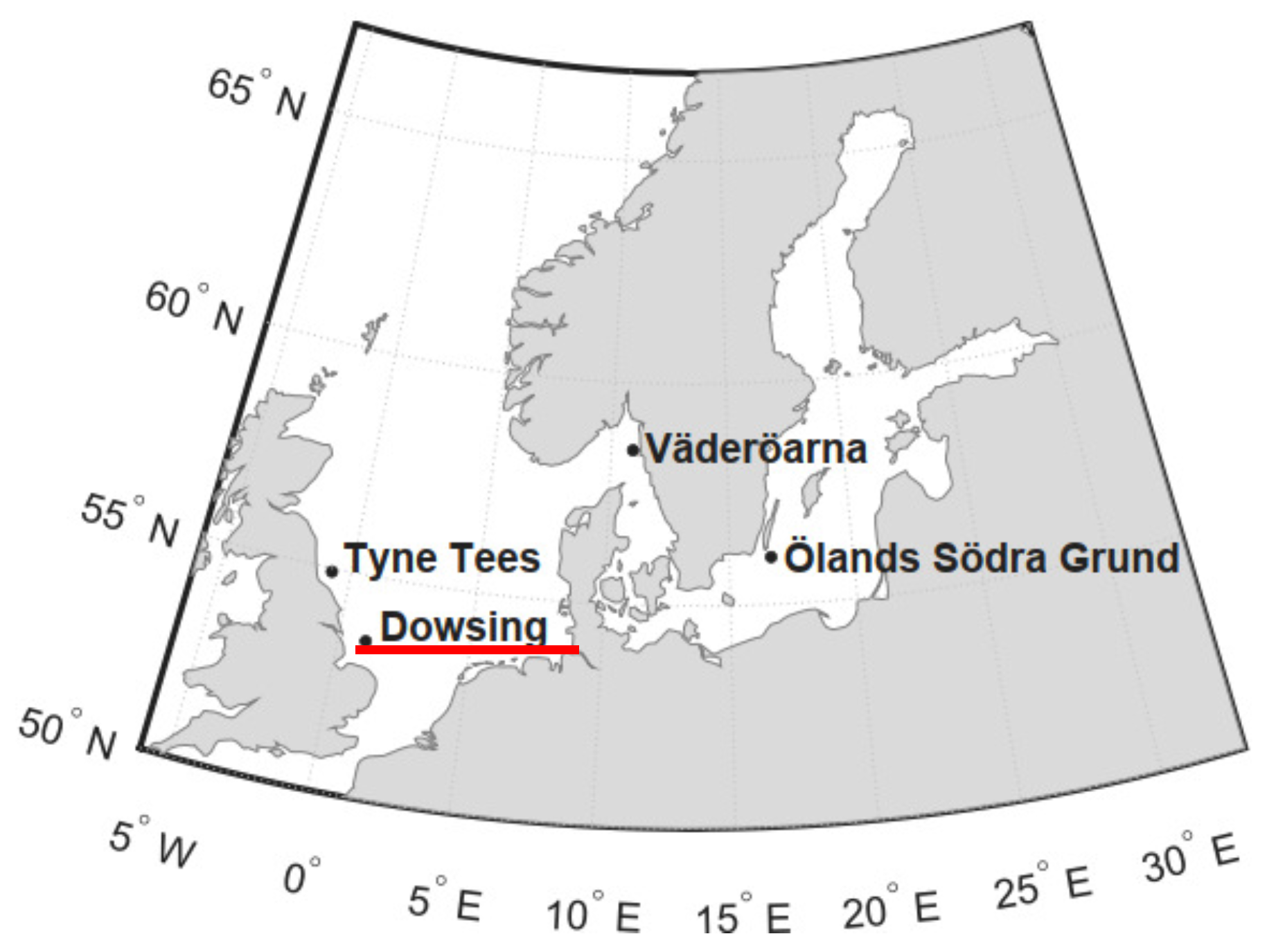
Figure 1.
The four selected sites examined in [
14] are shown. For the present study, the Dowsing site is selected, located in the North Sea; 56 km from the west coast of the United Kingdom, with water depth 22 m.
Figure 1.
The four selected sites examined in [
14] are shown. For the present study, the Dowsing site is selected, located in the North Sea; 56 km from the west coast of the United Kingdom, with water depth 22 m.
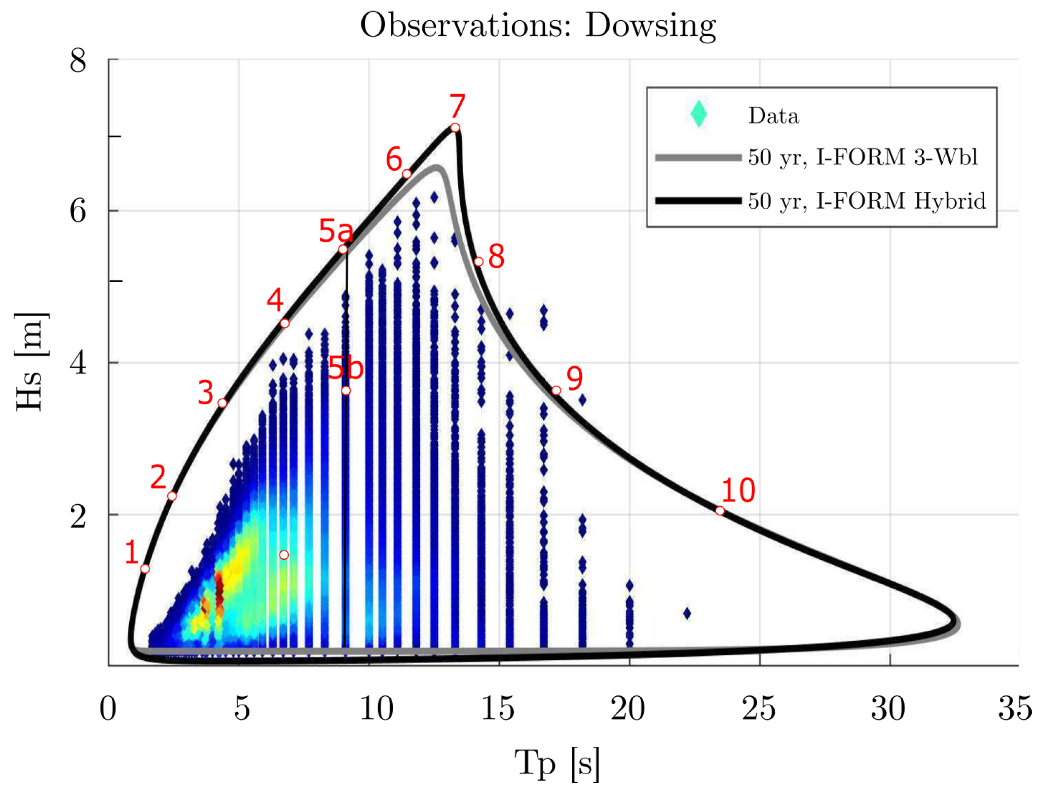
Figure 2.
The 50-year return period environmental contour for Dowsing site adapted from [
14]. The environmental contour, as calculated from I-FORM Hybrid method (black line), is utilized here. The contour line is discretized in 10 sea states plus one sea state (5b) inside the contour. Sea state 5b is selected so as to make the comparison between sea states with the same peak period,
, (5a vs. 5b) and sea states with the same significant wave height,
, (5b vs. 9). In the present study, sea states 5a, 5b, 6, 7, 8, and 9 are examined.
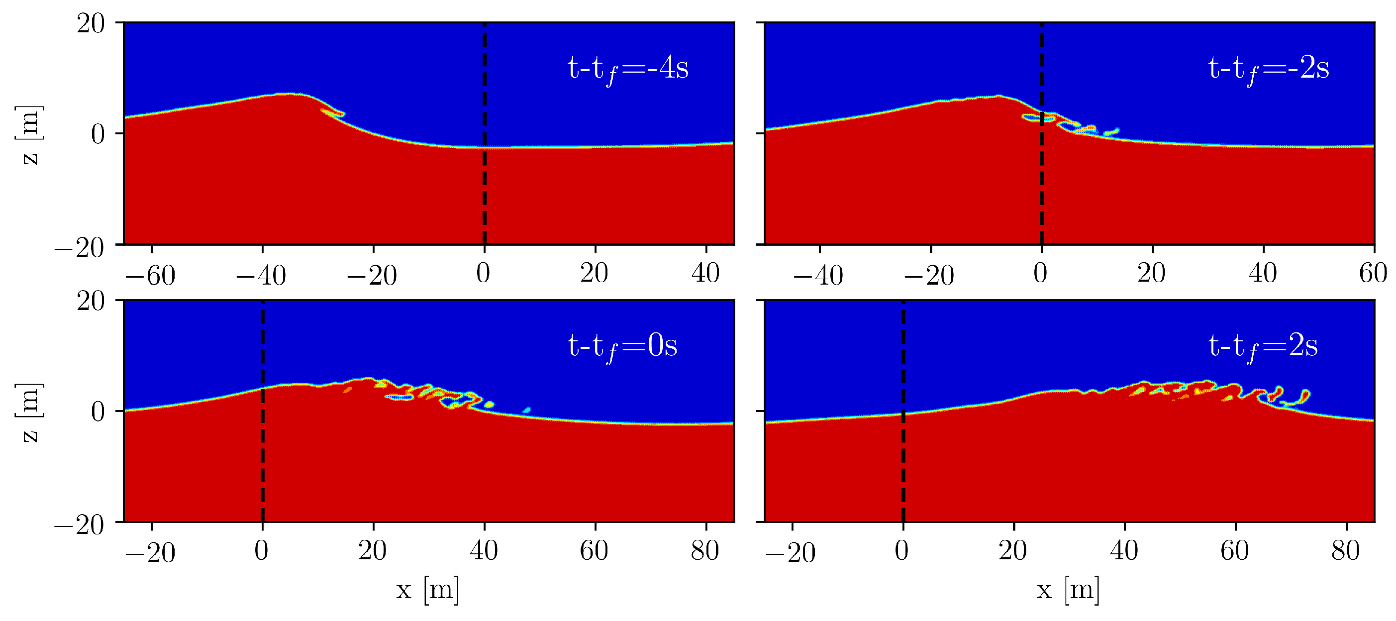
Figure 3.
Sea state 6. The focused wave is propagating in a two-dimensional numerical wave tank without the presence of the WEC. The wave propagation is captured for several time instances: (a) s, (b) s, (c) s (focal time), (d) s. The focal position is indicated by the dashed black line in which the WEC will be placed (horizontal direction x = 0 m).
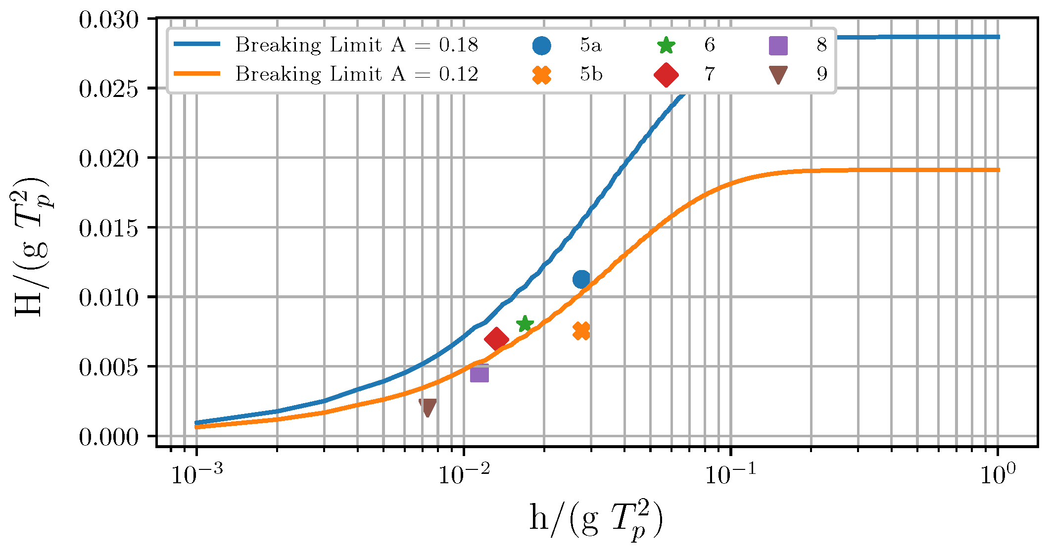
Figure 4.
The range of breaking criterion is shown. The breaking behaviour of the examined sea states is identified.
Figure 4.
The range of breaking criterion is shown. The breaking behaviour of the examined sea states is identified.
Figure 5.
Impact area on a slender cylinder due to slamming force, as adapted from [
43] with permission from Elsevier Ltd, UK, 2005.
Figure 5.
Impact area on a slender cylinder due to slamming force, as adapted from [
43] with permission from Elsevier Ltd, UK, 2005.
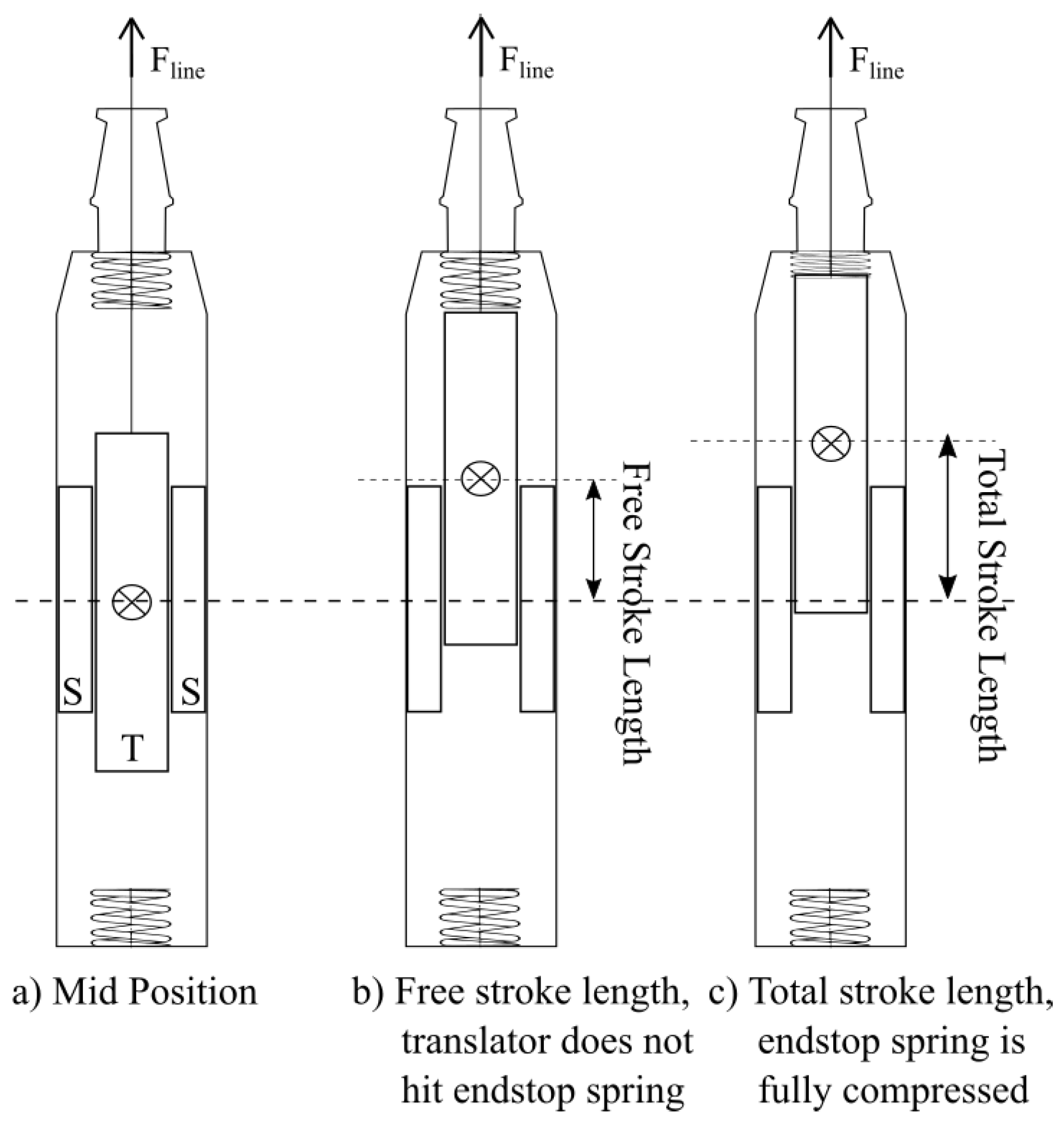
Figure 6.
Uppsala University WEC; schematic view of the direct-driven linear generator adapted from [
47] under the Creative Commons CC-BY license.
Figure 6.
Uppsala University WEC; schematic view of the direct-driven linear generator adapted from [
47] under the Creative Commons CC-BY license.
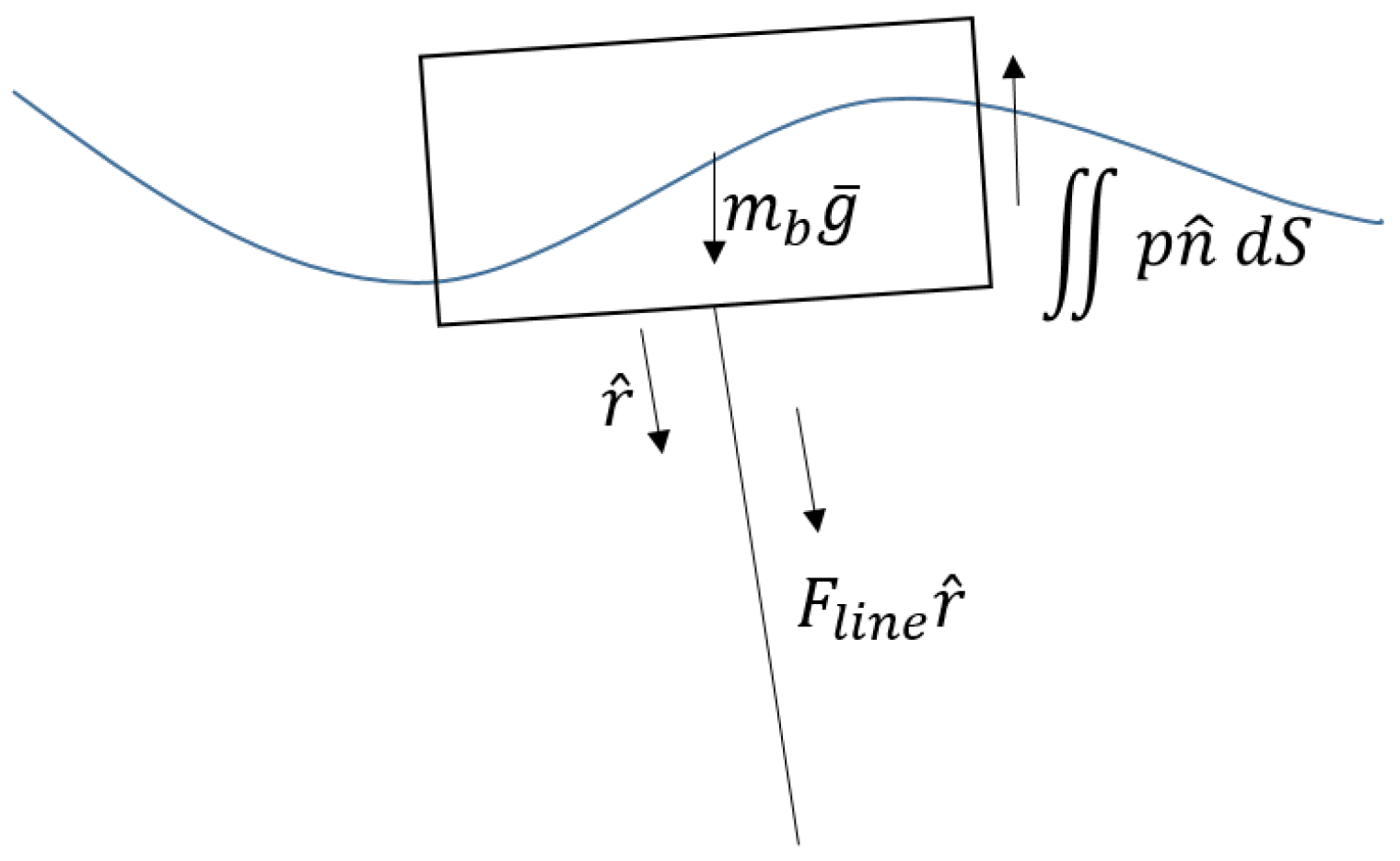
Figure 7.
The forces acting on the buoy are the sum of the hydrodynamic, gravitational and generator (
) forces adapted from [
47] under the Creative Commons CC-BY license.
Figure 7.
The forces acting on the buoy are the sum of the hydrodynamic, gravitational and generator (
) forces adapted from [
47] under the Creative Commons CC-BY license.
Figure 8.
The study for the numerical wave components selection is shown. The maximum wave height, , for sea state 5a using as a reference the maximum wave height obtained from the analytical solution, , is provided as a function of the wave components, N.
Figure 8.
The study for the numerical wave components selection is shown. The maximum wave height, , for sea state 5a using as a reference the maximum wave height obtained from the analytical solution, , is provided as a function of the wave components, N.
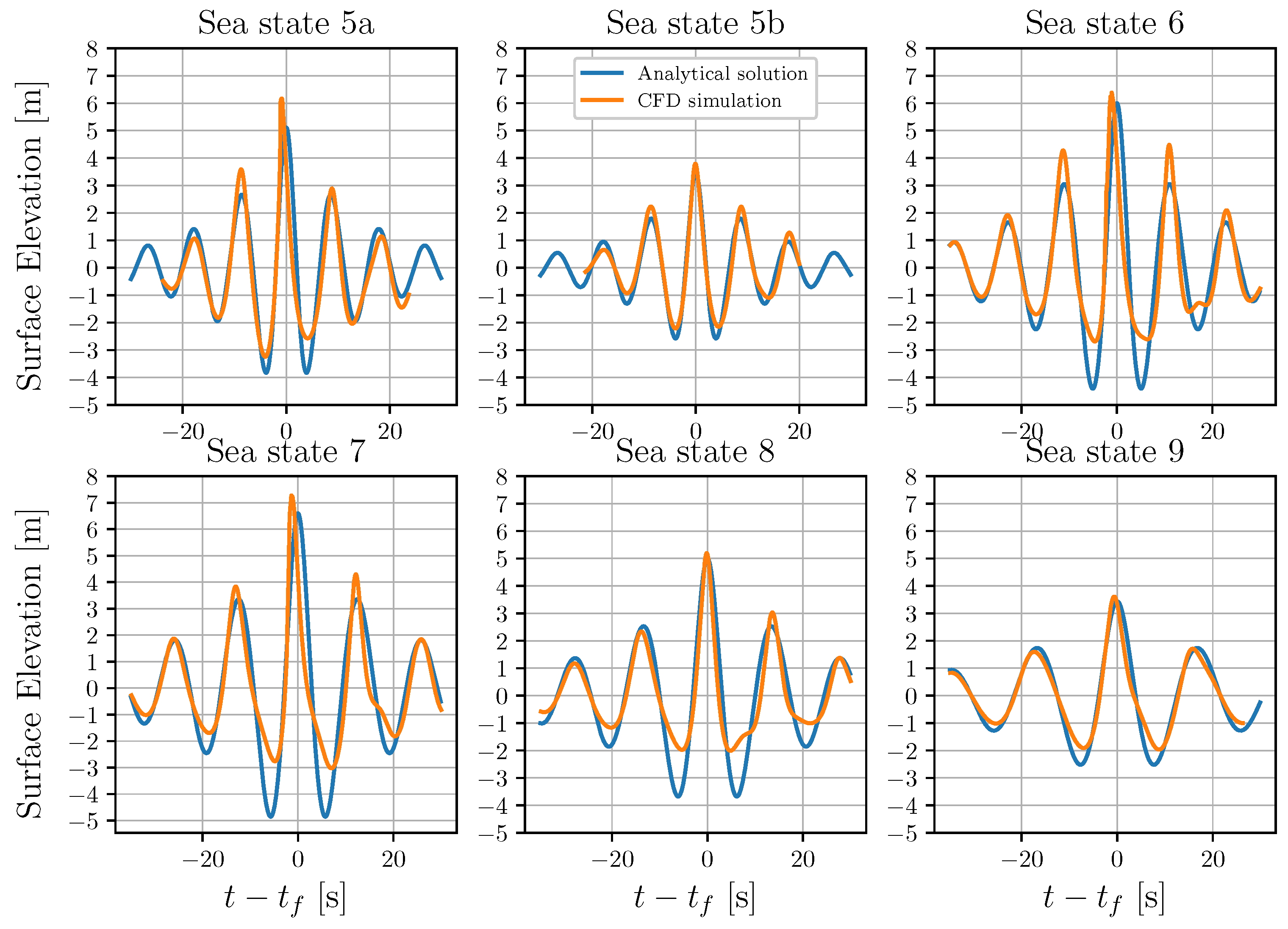
Figure 9.
Focused wave propagation at the focal point as given by the analytical solution and the numerical simulation. The analytical solution is based on NewWave theory, while CFD simulations calculate the wave propagation in a two-dimensional numerical wave tank.
Figure 9.
Focused wave propagation at the focal point as given by the analytical solution and the numerical simulation. The analytical solution is based on NewWave theory, while CFD simulations calculate the wave propagation in a two-dimensional numerical wave tank.
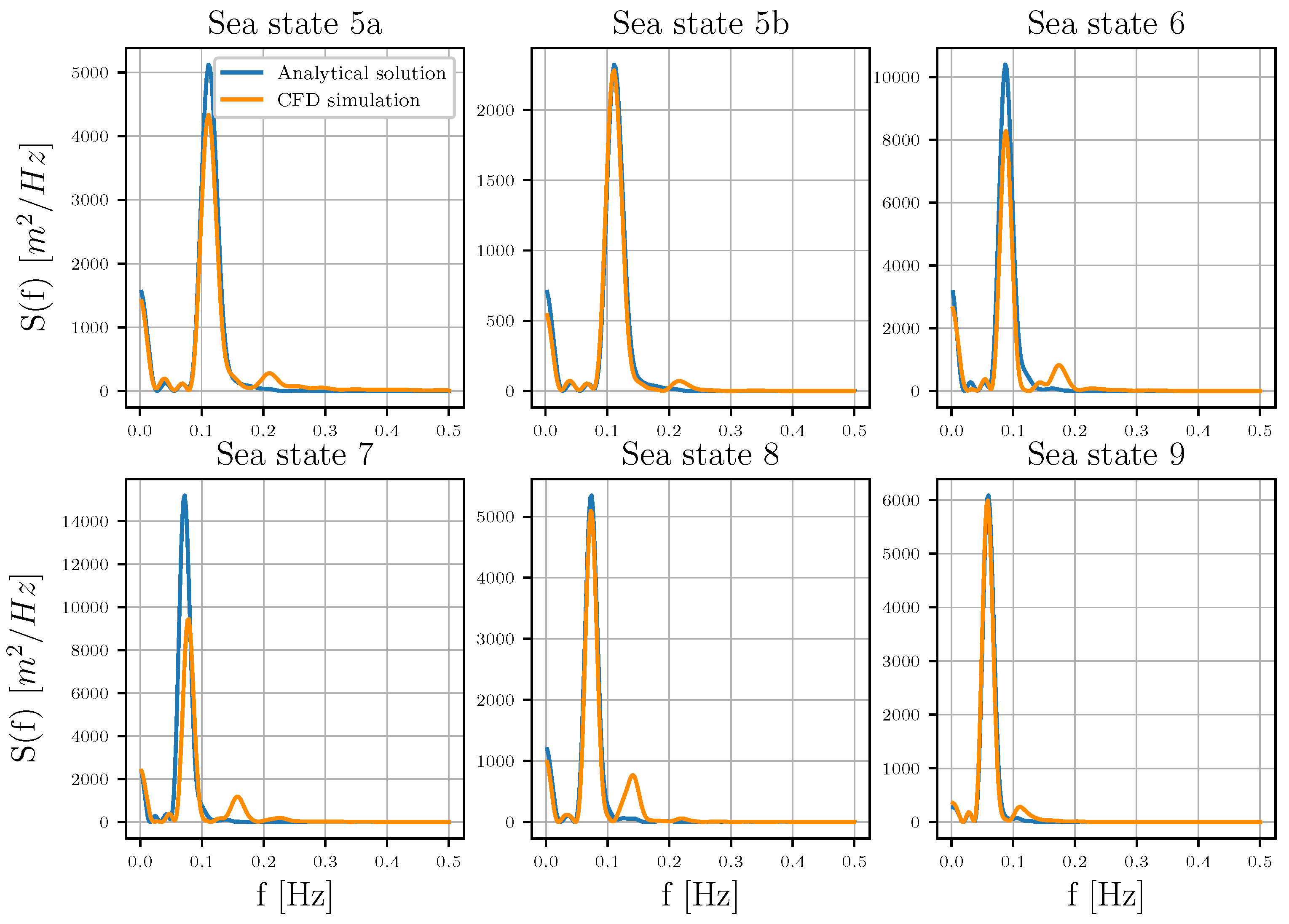
Figure 10.
Wave frequency spectra as obtained by Fourier transformation implemented in the time series shown in
Figure 9. The CFD solution is compared with the analytical.
Figure 10.
Wave frequency spectra as obtained by Fourier transformation implemented in the time series shown in
Figure 9. The CFD solution is compared with the analytical.
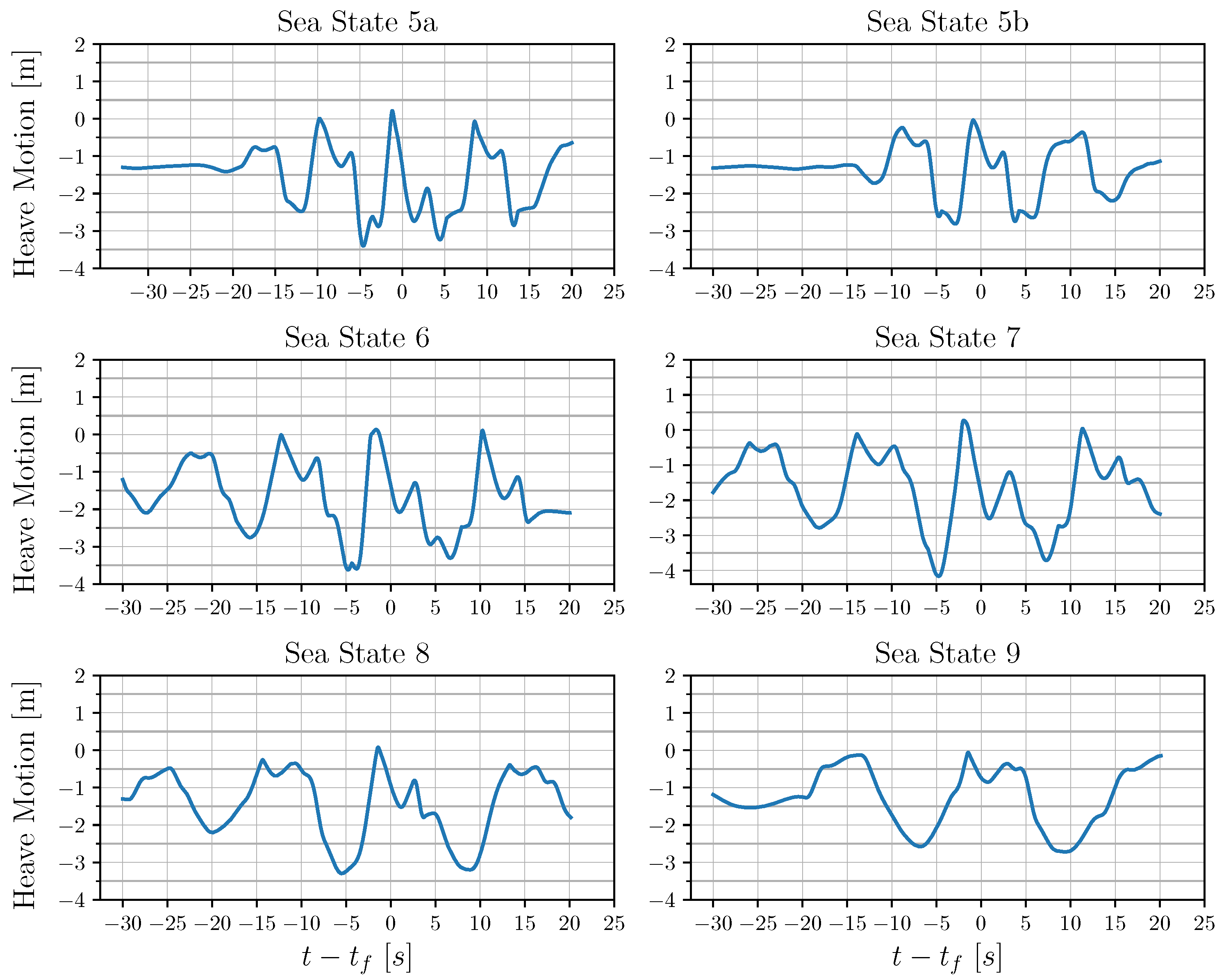
Figure 11.
For all the examined sea states, the heave response time series during the wave–structure interaction is shown.
Figure 11.
For all the examined sea states, the heave response time series during the wave–structure interaction is shown.
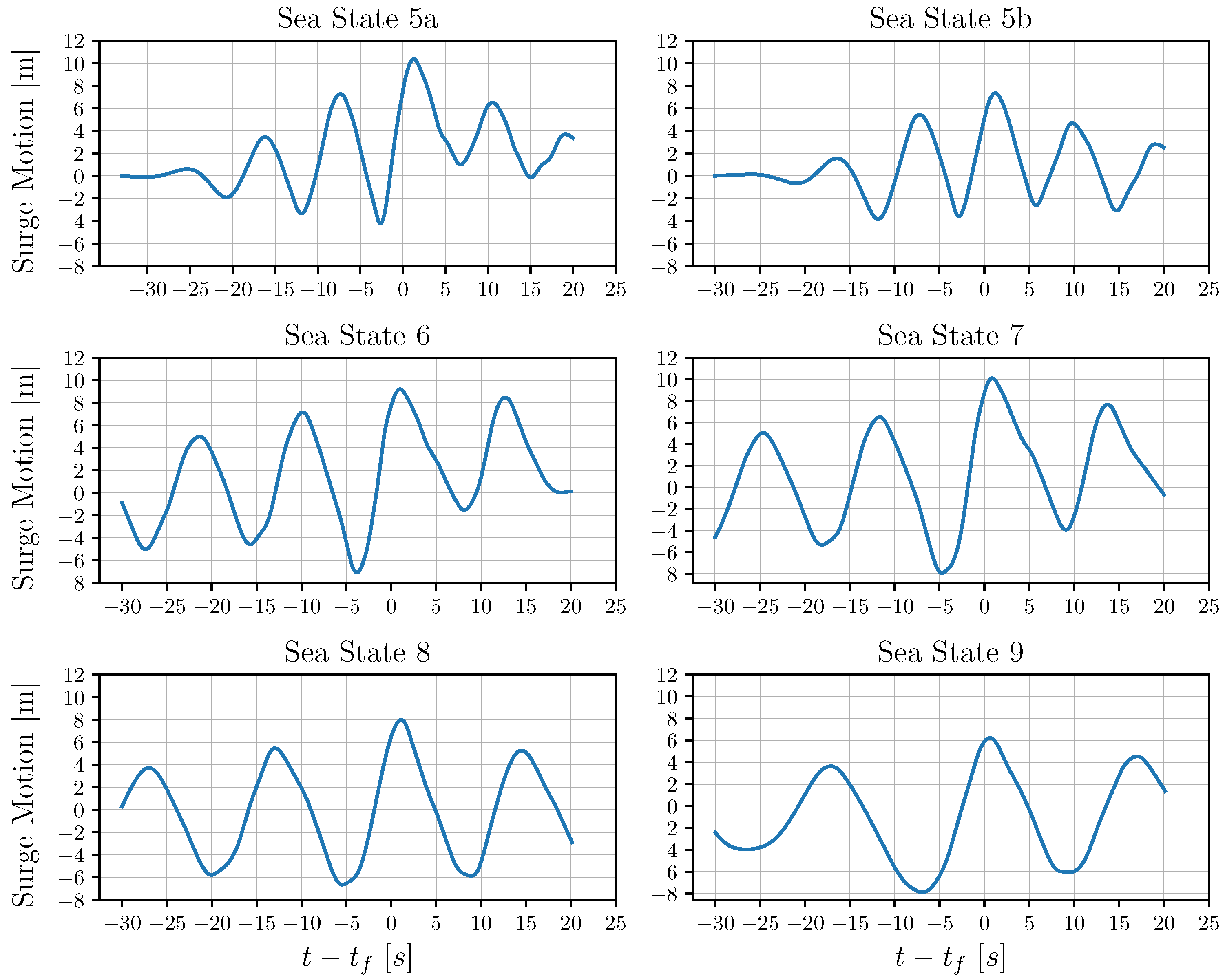
Figure 12.
For all the examined sea states, the surge response time series during the wave–structure interaction is shown.
Figure 12.
For all the examined sea states, the surge response time series during the wave–structure interaction is shown.
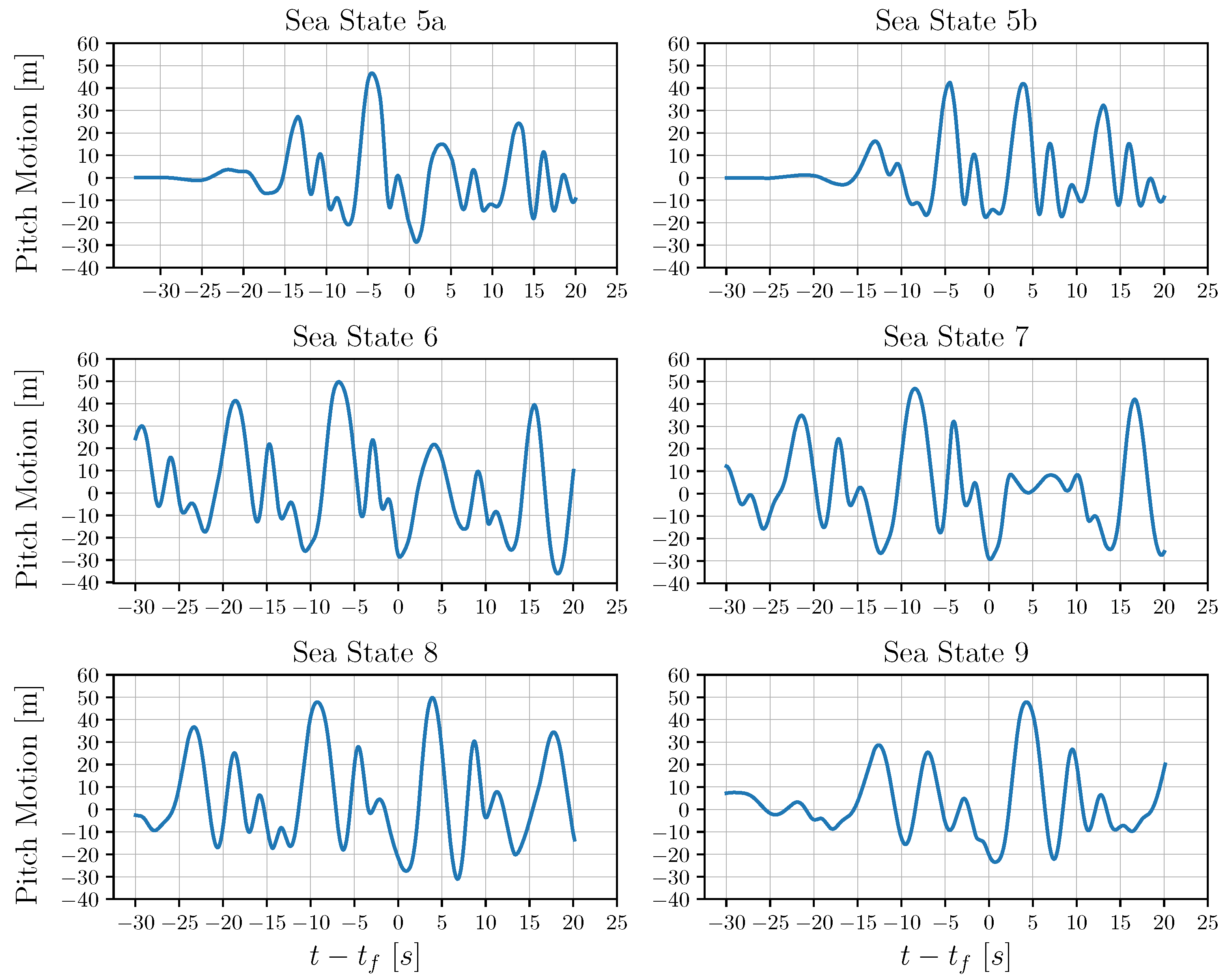
Figure 13.
For all the examined sea states, the pitch response time series during the wave–structure interaction is shown.
Figure 13.
For all the examined sea states, the pitch response time series during the wave–structure interaction is shown.
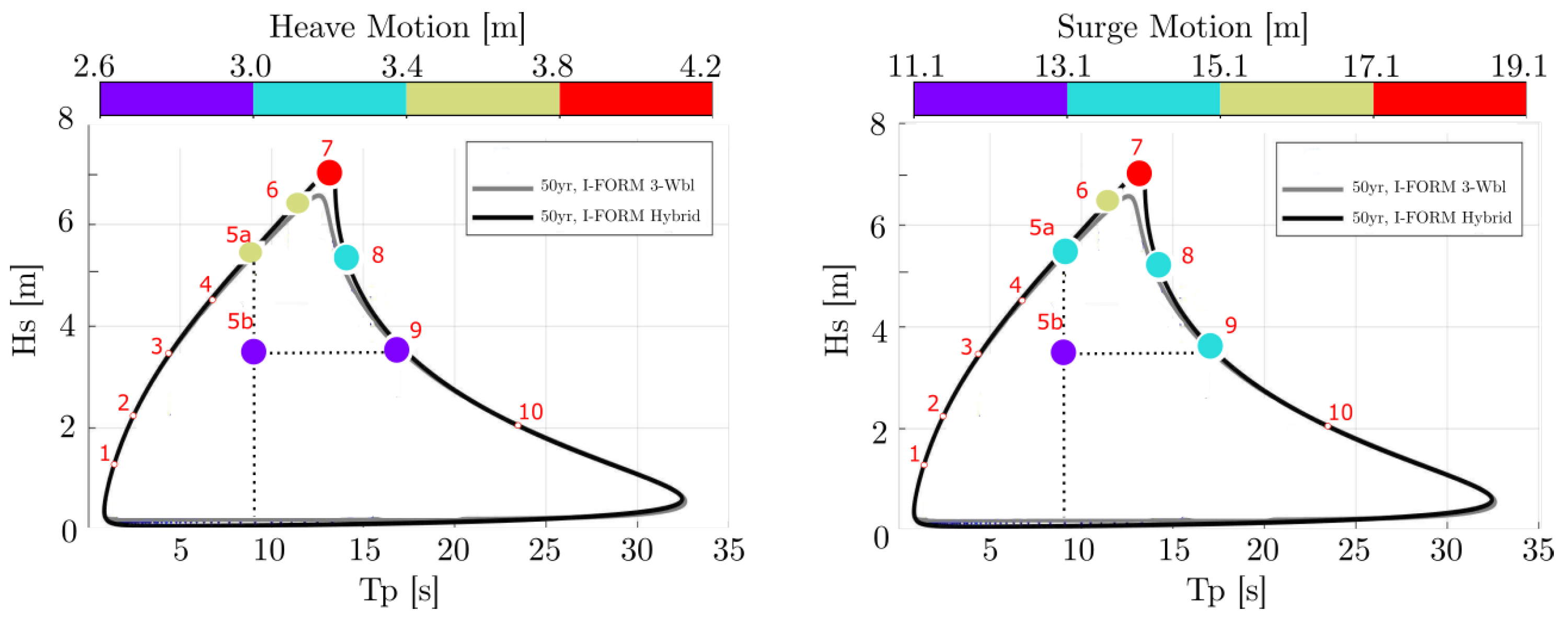
Figure 14.
Colormap visualization of the maximum heave response range (left) and maximum surge response range (right) along the environmental contour line.
Figure 14.
Colormap visualization of the maximum heave response range (left) and maximum surge response range (right) along the environmental contour line.
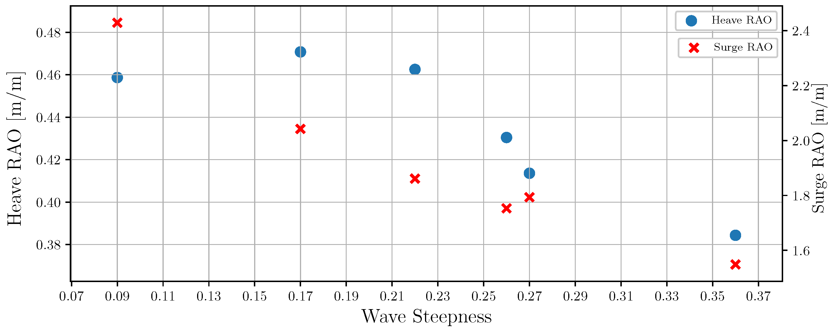
Figure 15.
For all the examined sea states, the heave and surge RAOs are shown as a function of the wave steepness.
Figure 15.
For all the examined sea states, the heave and surge RAOs are shown as a function of the wave steepness.
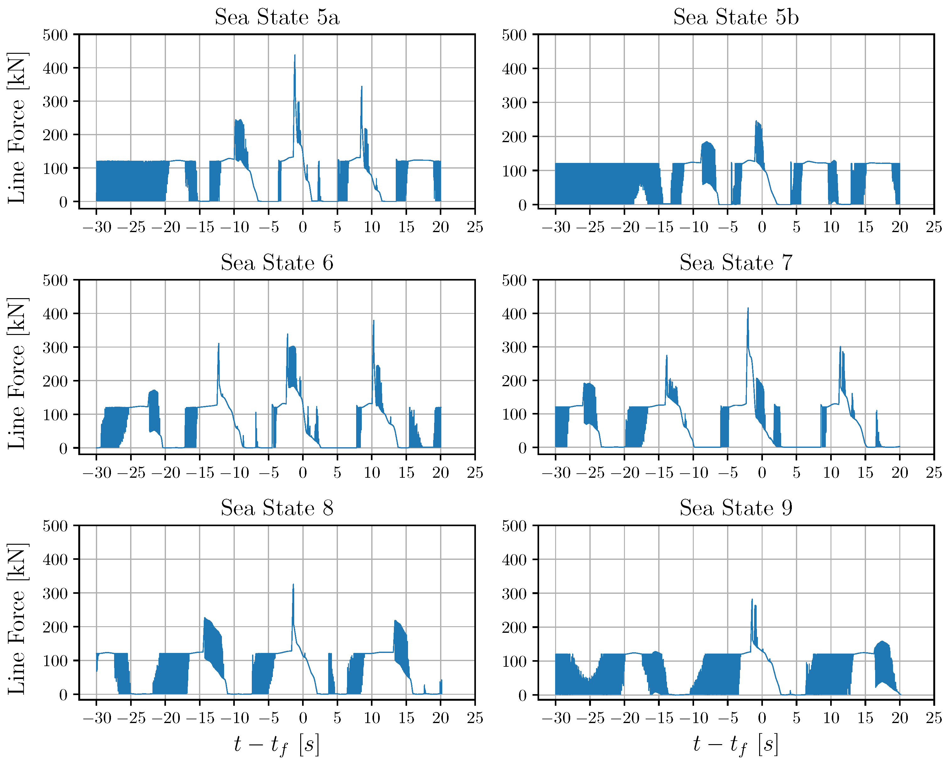
Figure 16.
For all the examined sea states, the time series of the connection line force during the wave–structure interaction is shown.
Figure 16.
For all the examined sea states, the time series of the connection line force during the wave–structure interaction is shown.
Figure 17.
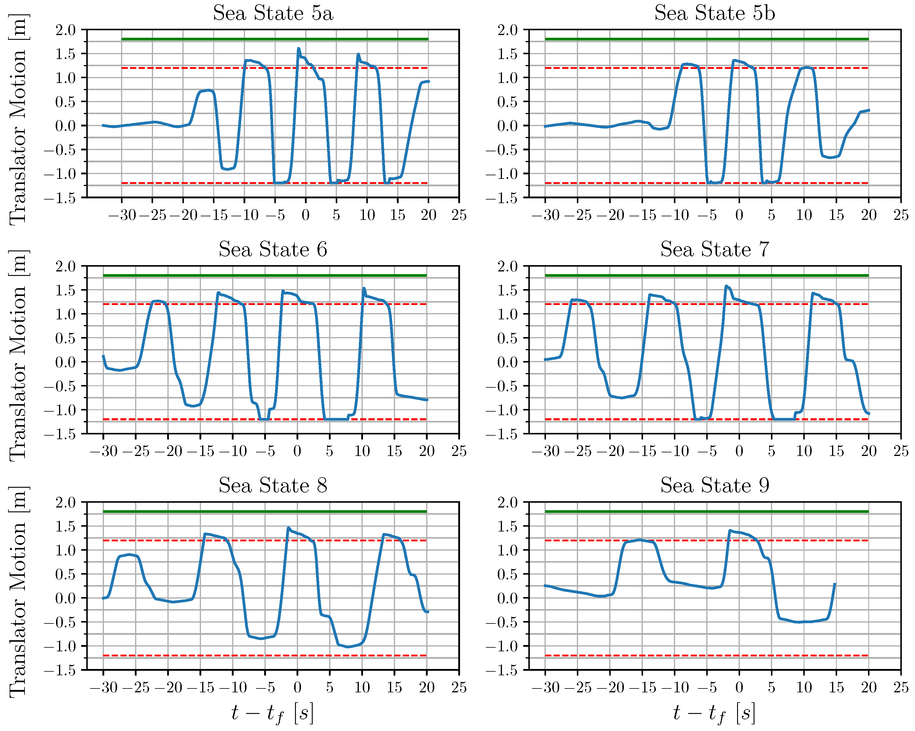
Time series of the translator’s motion during the wave–structure interaction, for all the examined sea states. The translator moves only vertically. The red dashed line indicates the upper and lower free stroke-length (1.2 m), the green line defines the maximum stroke-length (1.8 m). Once the translator exceeds the upper free-stroke length, the end-stop spring starts to compress. During the downward motion of the translator, once the lower free stroke-length of 1.2 m is exceeded, the translator stands on the bottom of the generator and the connection line with the buoy slacks. There is no lower end-stop spring in the present CFD restraint.
Figure 17.
Time series of the translator’s motion during the wave–structure interaction, for all the examined sea states. The translator moves only vertically. The red dashed line indicates the upper and lower free stroke-length (1.2 m), the green line defines the maximum stroke-length (1.8 m). Once the translator exceeds the upper free-stroke length, the end-stop spring starts to compress. During the downward motion of the translator, once the lower free stroke-length of 1.2 m is exceeded, the translator stands on the bottom of the generator and the connection line with the buoy slacks. There is no lower end-stop spring in the present CFD restraint.
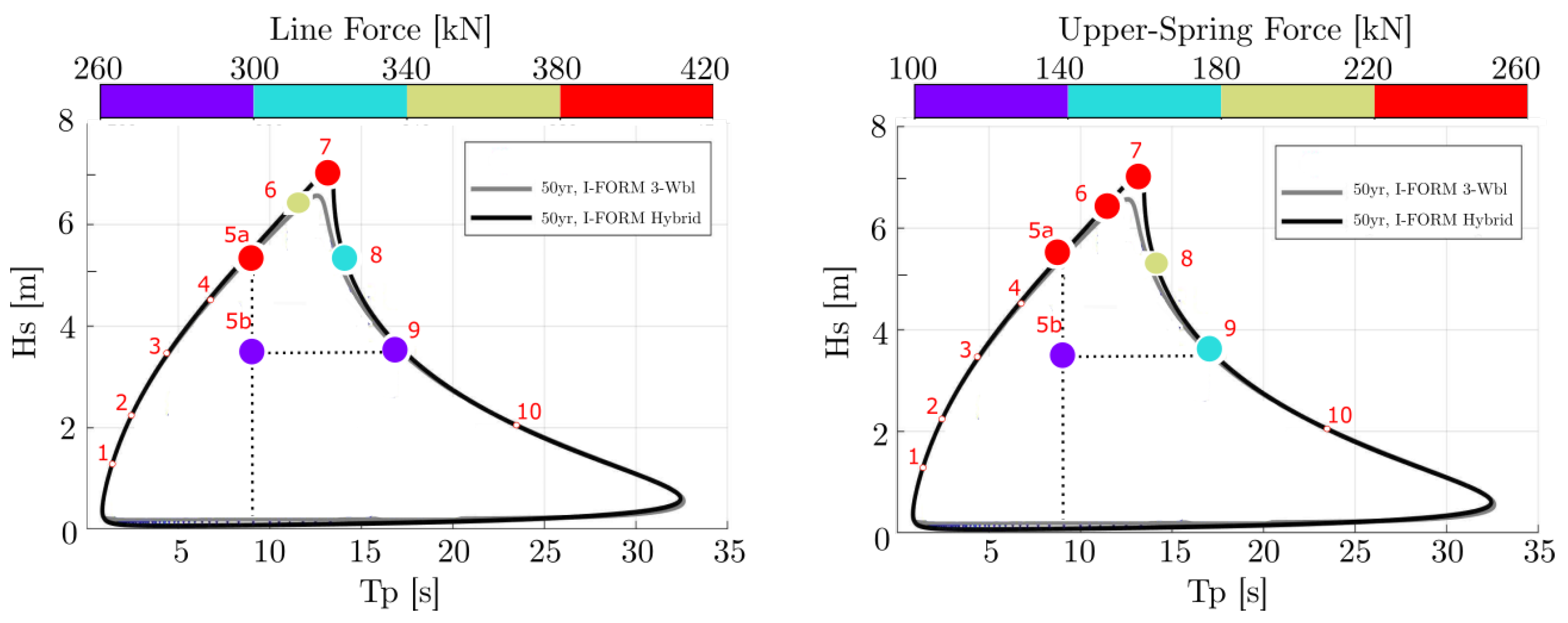
Figure 18.
Colormap visualization of the maximum force in the connection line (left) and the maximum force (right) on the upper end-stop spring along the environmental contour line.
Figure 18.
Colormap visualization of the maximum force in the connection line (left) and the maximum force (right) on the upper end-stop spring along the environmental contour line.
Figure 19.
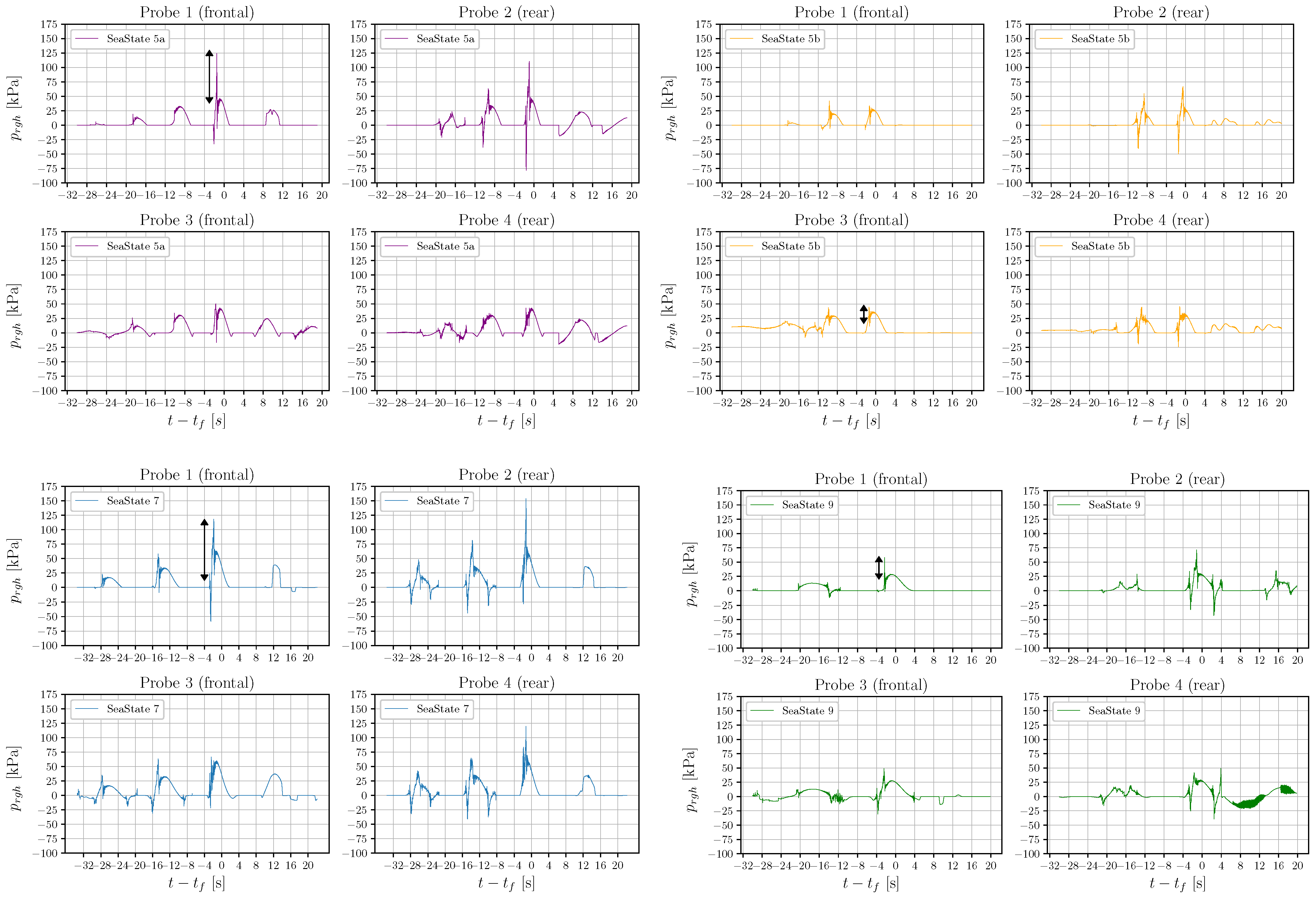
Pressure probes are mounted on the frontal and back part of the buoy. Probe 1 (frontal) and Probe 2 (rear) are located 0.24 m above SWL, whereas Probe 3 (frontal) and Probe 4 (rear) are located 0.97 m below the SWL. Time series of the pressure measured in each one probe is presented for sea states 5a (purple), 5b (orange), 7 (blue) and 9 (green). The black arrow indicates the slamming contribution.
Figure 19.
Pressure probes are mounted on the frontal and back part of the buoy. Probe 1 (frontal) and Probe 2 (rear) are located 0.24 m above SWL, whereas Probe 3 (frontal) and Probe 4 (rear) are located 0.97 m below the SWL. Time series of the pressure measured in each one probe is presented for sea states 5a (purple), 5b (orange), 7 (blue) and 9 (green). The black arrow indicates the slamming contribution.
Figure 20.
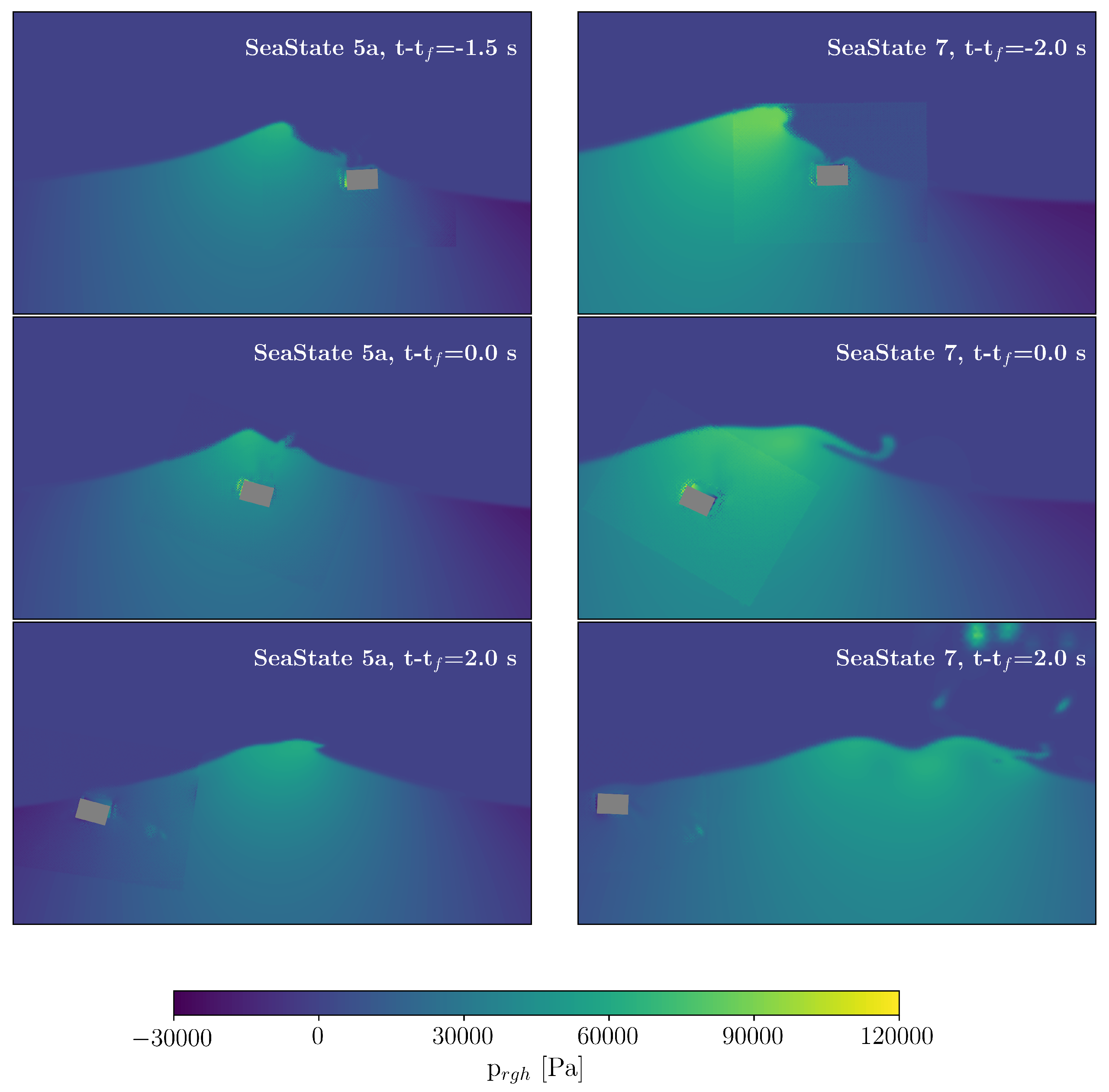
Wave–structure interaction at sea state 5a (left column) and sea state 7 (right column) as colored by the dynamic pressure, . The pictures on the top show the time instant in which the slamming occurs; the slamming happens 1.5 s and 2 s prior to the theoretical focus time for sea states 5a and 7, respectively. The pictures in the middle row depict the wave–structure interaction at the theoretical focused time, and the bottom pictures the wave–structure interaction as captured 2 s after the theoretical focus time. Both waves are breaking. At sea state 5a, the breaking phenomenon initiates just after the focused wave interacts with the buoy, whereas, at sea state 7, the wave starts to break in the frontal head of the buoy.
Figure 20.
Wave–structure interaction at sea state 5a (left column) and sea state 7 (right column) as colored by the dynamic pressure, . The pictures on the top show the time instant in which the slamming occurs; the slamming happens 1.5 s and 2 s prior to the theoretical focus time for sea states 5a and 7, respectively. The pictures in the middle row depict the wave–structure interaction at the theoretical focused time, and the bottom pictures the wave–structure interaction as captured 2 s after the theoretical focus time. Both waves are breaking. At sea state 5a, the breaking phenomenon initiates just after the focused wave interacts with the buoy, whereas, at sea state 7, the wave starts to break in the frontal head of the buoy.
Figure 21.
Wave–structure interaction at the sea states 5b (left column) and 9 (right column) as colored by the dynamic pressure, . The pictures show the motion a few seconds before the focusing time ( s, on the top) and at the focusing time ( s, at the bottom).
Figure 21.
Wave–structure interaction at the sea states 5b (left column) and 9 (right column) as colored by the dynamic pressure, . The pictures show the motion a few seconds before the focusing time ( s, on the top) and at the focusing time ( s, at the bottom).
Figure 22.
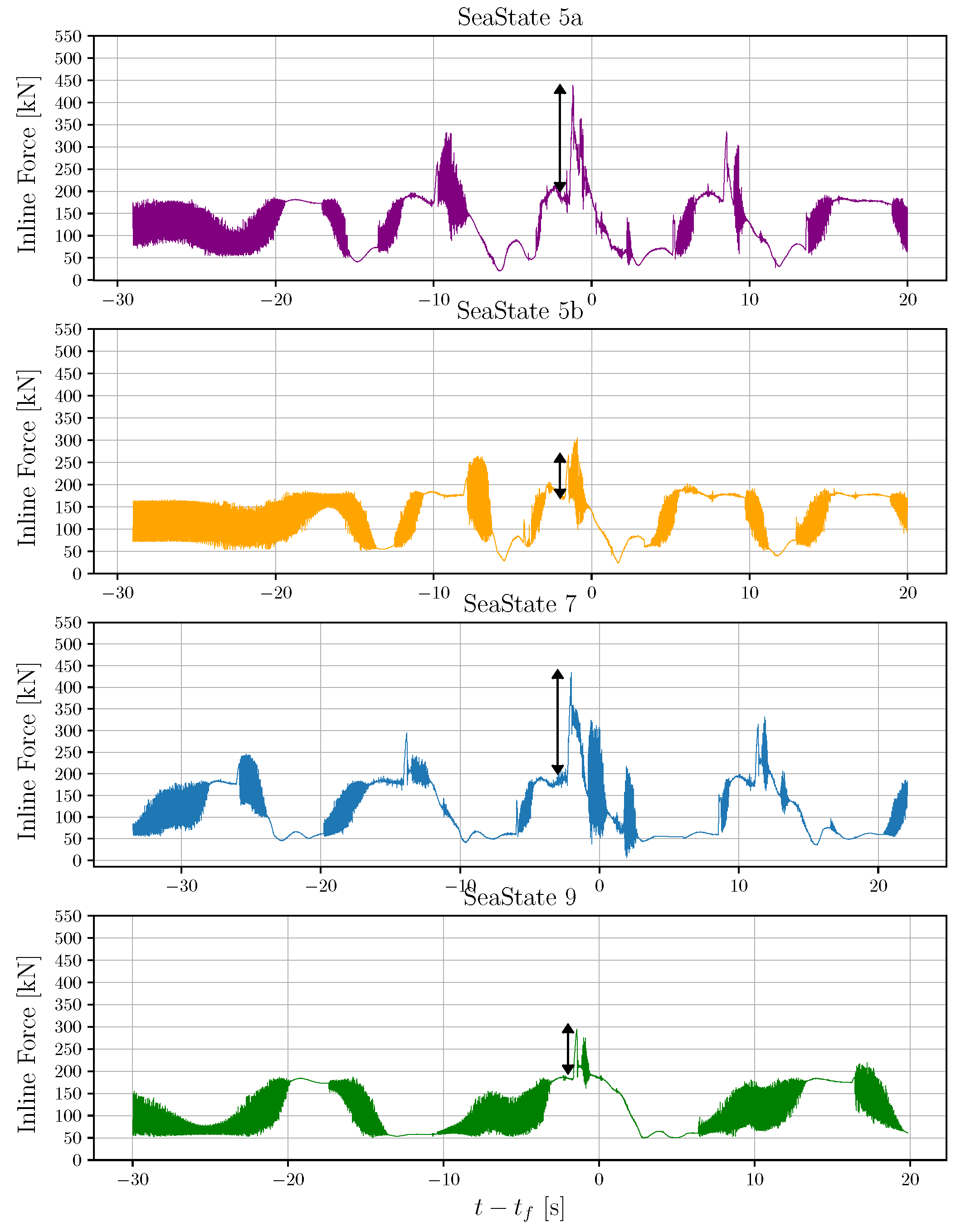
Inline (excitation) force acting on the buoy during sea states 5a (purple), 5b (orange), 7 (blue) and 9 (green) according to CFD solution. The force is calculated by the integration of the normal pressure on the buoy surface. The black arrow indicates the contribution of the slamming force.
Figure 22.
Inline (excitation) force acting on the buoy during sea states 5a (purple), 5b (orange), 7 (blue) and 9 (green) according to CFD solution. The force is calculated by the integration of the normal pressure on the buoy surface. The black arrow indicates the contribution of the slamming force.
Table 1.
Characteristics of the sea states 5 to 9, along the Dowsing environmental contour. and are the significant wave height and peak period, respectively. The maximum theoretical crest amplitude of the focused wave, , is calculated following the New Wave theory. The wave height of the focus wave, H, is defined as the height between the maximum wave crest and the minimum wave trough. is the peak wave length, the parameter measures the steepness of the waves, where corresponds to the peak frequency, and is the Keulegan–Carpenter number.
| | | | | | | |
|---|
| 5a | 5.5 | 9.0 | 5.1 | 9.0 | 108 | 0.29 | 10.2 |
| 5b | 3.7 | 9.0 | 3.4 | 6.0 | 108 | 0.20 | 6.9 |
| 6 | 6.5 | 11.5 | 6.0 | 10.4 | 150 | 0.25 | 12.0 |
| 7 | 7.1 | 13.0 | 6.6 | 11.5 | 174 | 0.24 | 13.2 |
| 8 | 5.4 | 14.0 | 5.0 | 8.7 | 190 | 0.17 | 10.0 |
| 9 | 3.7 | 17.5 | 3.4 | 6.0 | 244 | 0.09 | 6.9 |
Table 2.
Evaluation of NWT’s length downstream the body and NWT’s width. In terms of the length, four lengths have been considered: , , , . For the width, three cases have been considered: 50 m, 100 m, 170 m. The RMSE value for the surface elevation at the buoy’s position is calculated, having as reference the case for and 170 m for the evaluation of the length and width, respectively.
| | | | |
|---|
| 50 | 0.7 | | 2.25 | 0.25 |
| 100 | 0.5 | | 0.41 | 0.019 |
| - | - | | 0.046 | 0.0003 |
Table 3.
Boundary conditions of the computational domain.
Table 3.
Boundary conditions of the computational domain.
| Variables | Inlet/Outlet | Seabed | Atmosphere | SideWalls |
|---|
| alpha.water | waveAlpha */zeroGradient | zeroGradient | inletOutlet | zeroGradient |
| Velocity | waveVelocity * | slip | pressureInletOutletVelocity | slip |
| Pressure | fixedFluxPressure | zeroGradient | totalPressure | fixedFluxPressure |
| k | zeroGradient | kqRWallFunction | inletOutlet | slip |
| zeroGradient | omegaWallfunction | inletOutlet | slip |
Table 4.
Spatial convergence study for the steepest wave (sea state 5a). The spatial discretizetion is evaluated through the numerical uncertainty U, for the maximum wave crest and the deepest wave trough, .
Table 4.
Spatial convergence study for the steepest wave (sea state 5a). The spatial discretizetion is evaluated through the numerical uncertainty U, for the maximum wave crest and the deepest wave trough, .
| | | | | |
|---|
| Coarse | 0.425 | 12 | 2.25 | 0.82 |
| Medium | 0.30 | 17 | 0.41 | 0.73 |
| Fine | 0.213 | 24 | 0.046 | 0.61 |
| Finest | 0.15 | 34 | 0.046 | 0.56 |
Table 5.
Steepness () and maximum wave height () for the focused wave group as calculated by the NewWave theory and the numerical solution (CFD).
Table 5.
Steepness () and maximum wave height () for the focused wave group as calculated by the NewWave theory and the numerical solution (CFD).
| | | | | | | |
|---|
| 5a | 0.36 | 0.29 | 9.4 | 9.0 | 12.4 | 10.2 |
| 5b | 0.22 | 0.20 | 6.0 | 6.0 | 7.6 | 6.9 |
| 6 | 0.27 | 0.25 | 9.0 | 10.4 | 12.8 | 12.0 |
| 7 | 0.26 | 0.24 | 10.3 | 11.5 | 14.5 | 13.2 |
| 8 | 0.17 | 0.17 | 7.2 | 8.7 | 10.4 | 10.0 |
| 9 | 0.09 | 0.09 | 5.8 | 6.0 | 7.2 | 6.9 |
Table 6.
Induced-pressure on the buoy due to the short impact of the wave–structure interaction as it is given from CFD simulations,
, and, as calculated from the Equation (
25),
. The relative velocity,
v, as calculated from the CFD simulations, is also given. The deviation between the theoretical and the numerical pressure is provided.
| Sea State | [kPa] | v [m/s] | [kPa] | [%] |
|---|
| 5a | 80 | 6.2 | 99 | 23.7 |
| 5b | 20 | 2.9 | 26.4 | 32 |
| 7 | 95 | 6.6 | 112 | 18 |
| 9 | 28 | 3.5 | 38.5 | 37.4 |
Table 7.
The slamming force () as calculated from the CFD simulations, the percentage contribution of slamming force () in the total inline force, and the factor identifying the impact area on the buoy.
Table 7.
The slamming force () as calculated from the CFD simulations, the percentage contribution of slamming force () in the total inline force, and the factor identifying the impact area on the buoy.
| Sea State | [kN] | | |
|---|
| 5a | 264 | 139 | 0.08 |
| 5b | 90 | 47 | 0.11 |
| 7 | 235 | 124 | 0.06 |
| 9 | 115 | 60.5 | 0.10 |


 ,
, 


