Study of the Operating Characteristics for the High-Speed Water Jet Pump Installed on the Underwater Vehicle with Different Cruising Speeds

Abstract

Due to the higher propulsive efficiency, lesser vibration, and better maneuverability, the water jet pump is widely applied to high-speed underwater vehicles. By taking a newly developed water jet pump system as the object, the corresponding underwater vehicle’s operating characteristics affected by different cruising speeds (15.43, 30.86, and 52.47 m/s) were investigated. The steady results reply that the cruising speed increase will result in the decline of the overall performances comprised of the head, the efficiency, the thrust, and the power. While, by using different analyzing methods, the unsteady results are listed as follows: (1) The energy loss theory denotes that the increasing cruising speed promoted the kinetic energy diffusion from the Reynolds stress and viscous stress and depress the turbulent kinetic energy production and the viscous dissipation. (2) The statistical PLS method reveals that the tip load effect on the leakage flow becomes weaker when the cruising speed becomes larger, while the effect from the scraping pressure has a completely opposite trend. (3) Further unsteady analysis implies that the increasing cruising speed makes the pressure pulsation larger and makes the radial force, the axial force, and the cloudy cavity size smaller.

1. Introduction

The waterjet pump has been widely applied to high-speed ferries and military amphibian vehicles due to its higher propulsive efficiency, lesser vibration, and better maneuverability [1]. As for the working process, the water around the underwater vehicle is absorbed into the intake duct and worked with the rotating waterjet pump to generate the axial thrust. With the application of the reacting force and the steering device, the underwater vehicle can move forward and change its cruising direction [2,3].

To investigate the operating characteristics of the underwater vehicle, numerous effects, including the simulation and the experiment, have been tried by previous scholars. As early as the 1990s, the International Towing Tank Conference (ITTC) proposed the momentum and energy flux theory [4], and then based on this method, Bulten et al. [5] and Delaney et al. [6] used the summation of wall forces or the momentum balance to predict the pump thrust. Though the external performances could be approximately obtained in related studies, the 3D flow for the underwater vehicle cannot be clearly presented. To make for the shortage, Ding et al. [7] added the additional user-defined scalar (UDS) equation into the fluent software to simulate the flow ingested into the intake duct of the propulsion pump. Later, with the development of the computational fluid dynamic (CFD) technique, many detailed investigations about the local performances have been conducted; for example, Luo et al. [8] and Cao et al. [9] has analyzed the energy performance and pressure fluctuations for a waterjet pump under different inflow conditions; Lu et al. [10] has attempted to study the tip clearance size of the pumpjet propeller based on the unsteady Reynolds-averaged Navier–Stokes equations; Aldas et al. [11] has used CFD to evaluate the effects of the surface roughness on the waterjet pump performance.

Apart from the simulating approach, many scholars tried to use the experimental approach to take a detailed investigation. Esch et al. [12] experimentally and numerically studied the quantitative relationship between the instability from the head curve and the unsteady forces caused by the blade tip clearance. Bonaiuti et al. [13] have designed out a waterjet pump with a developed inverse design method and tested the pump performance. Due to the limitations and shortcomings in the experiment, it is difficult to directly evaluate the whole performance of the underwater vehicle along with the waterjet pump in the towing tank. Even though some scholars still tried to make a breakthrough, for instance, by taking the entire body of the low-speed smart ship as the study target, Jiang et al. [14] proposed a vector control technology to improve maneuverability. Since the underwater vehicle, along with the water jet pump, has a much higher cruising speed, it is difficult to directly evaluate the water jet propulsion performance in the towing tank. Thus, similar to ref. [8,9,15], the validated numerical approach is still taken as the tool to evaluate the performance of the underwater vehicle with a high-speed water jet pump system.

According to the previous studies, it was found that the specific details and flow mechanism for partial components, such as the intake duct and the rotating impeller, have been clarified; however, there still exists some limitations. First of all, the rotating speed of the pump system is rather low in related studies, while the flow mechanism analysis with the high-speed water jet propulsion pump is urgent. When the pump’s rotating speed gets larger, the pump performance will drop sharply, and the corresponding inner flow becomes complex [10]. Moreover, design and inner flow analysis about the specific hydraulic component are the main focus, and there is a lack of study about the matching study between the waterjet pump and the whole navigating body.

Overall, to make up for the lack of adaptive study about the underwater vehicle installed with the high-speed water jet propulsion pump, this study takes a newly developed water jet pump system whose specific speed is close to the critical specific speed as the study object. Moreover, considering the influence of the underwater vehicle’s body and the external environment flow, effects of the cruising speeds on the underwater vehicle and the installed water jet pump are evaluated. Accordingly, the study here is mainly organized as follows: Part 2 illustrates the numerical approach, including the boundary condition and the turbulence model; Part 3 analyzes the operating characteristics of the underwater vehicle with a newly developed high-speed waterjet pump under different cruising speeds; Part 4 provides conclusions.

2. Numerical Approach

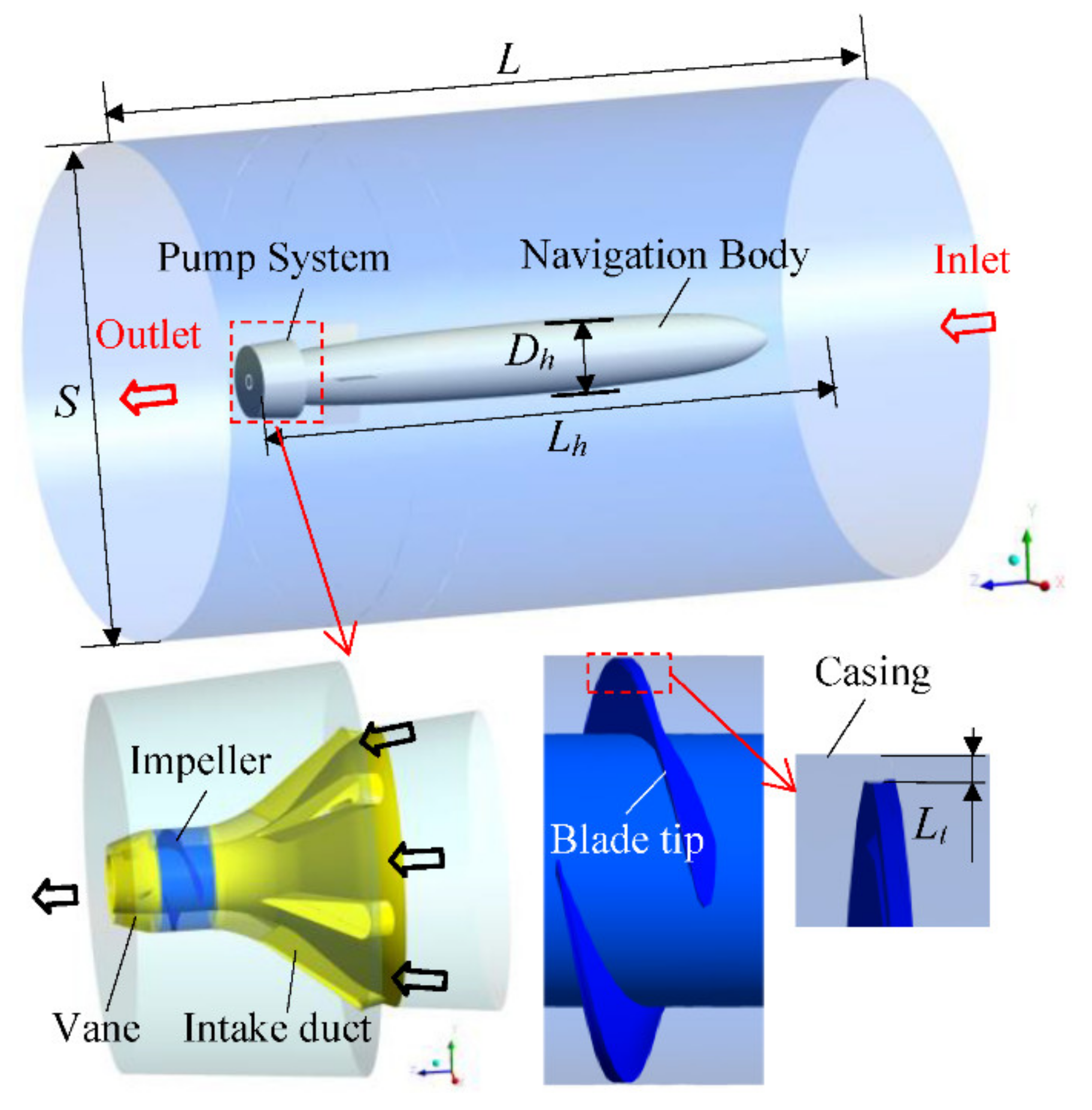
2.1. Computational Domain and Boundary Conditions

The underwater vehicle installed with the newly developed high-speed water jet pump is presented in Figure 1. In the figure, the underwater vehicle was mainly comprised of the navigation body, the pump system. As for the pump system, its main hydraulic components were the intake duct, the impeller, and the vane. The main size information of the underwater vehicle listed as the length of the whole computational domain L equals 6.5 m; the diameter of the simulation domain equals 4.0 m; the length of the underwater vehicle L_h was 4.35 m; the maximum diameter of the underwater vehicle D_h was to 0.38 m. Additionally, to avoid the scraping between the rotating blade and the static casing, the blade tip clearance L_t was set to be 0.2 mm.

As for the underwater vehicle, its corresponding design cruising speed was Ud = 60 kn. The rotating speed for the pump system was designed to be 17,500 RPM. At the design cruising speed, the design mass flow was Q_d = 294 kg/s, and the head was H_d = 114 m. The diving depth of the underwater vehicle was supposed to be h = 50 m. With these known operating variables, the specific speed ns of the impeller were calculated as 980 according to ref. [16,17,18], which belongs to the high-speed pump [10].

The turbulent flows were simulated with the code embodied in the ANSYS-CFX solver. Regarding the operating conditions and the setting options of the solver, the boundary conditions for the computational domain were given as the velocities of the inlet flow were set to be 0.5 Ud, 1.0 Ud and 1.7 Ud separately; the pressure at the outlet was set to be 490,000 Pa according to the formula ρgh; the interfaces between the static components were set to be the “none” mode; the interfaces between the static component were set to be the “frozen rotor” mode at the steady simulating stage, while they were set to be the “transient rotor-stator” mode at the unsteady simulating stage.

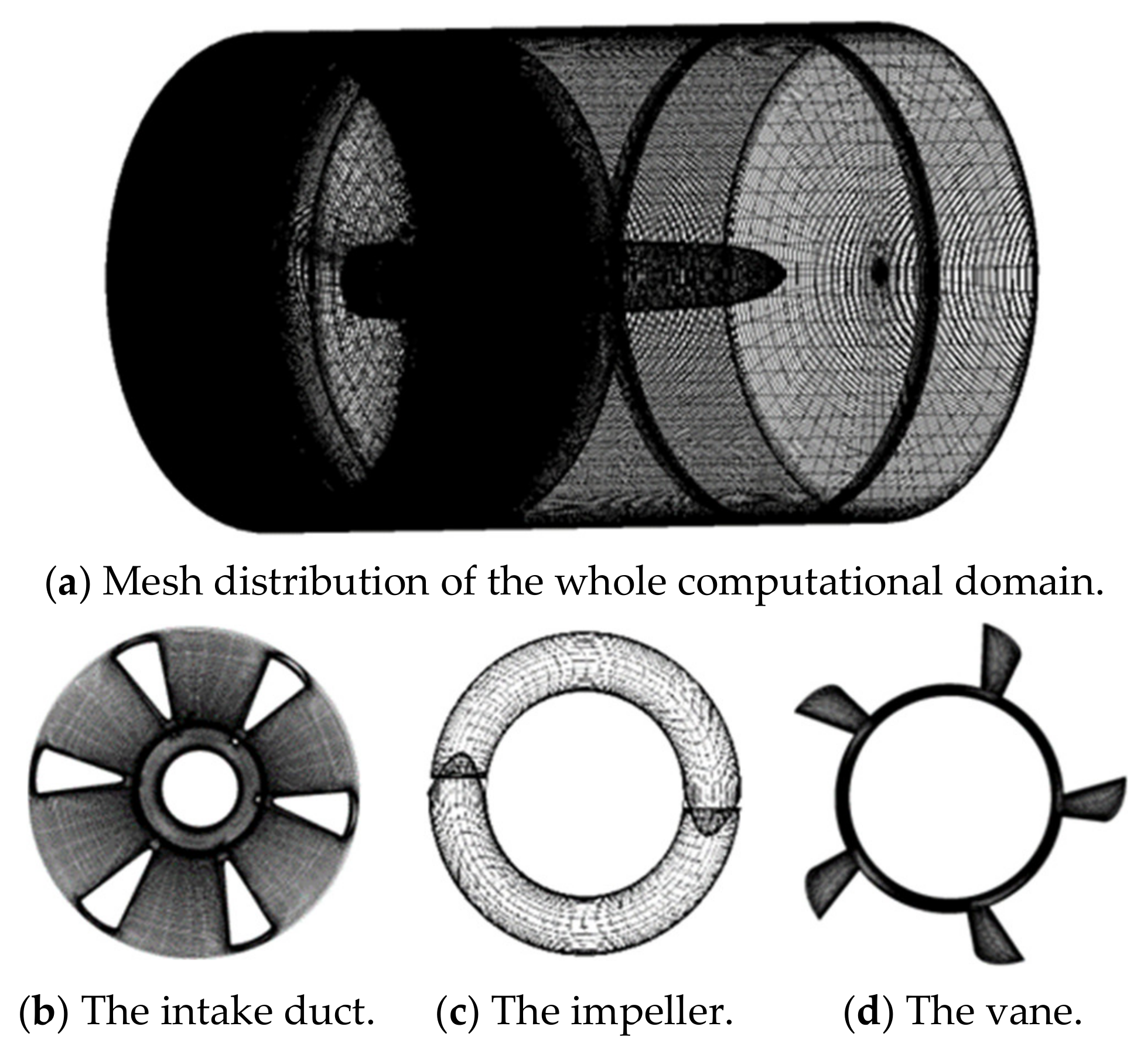
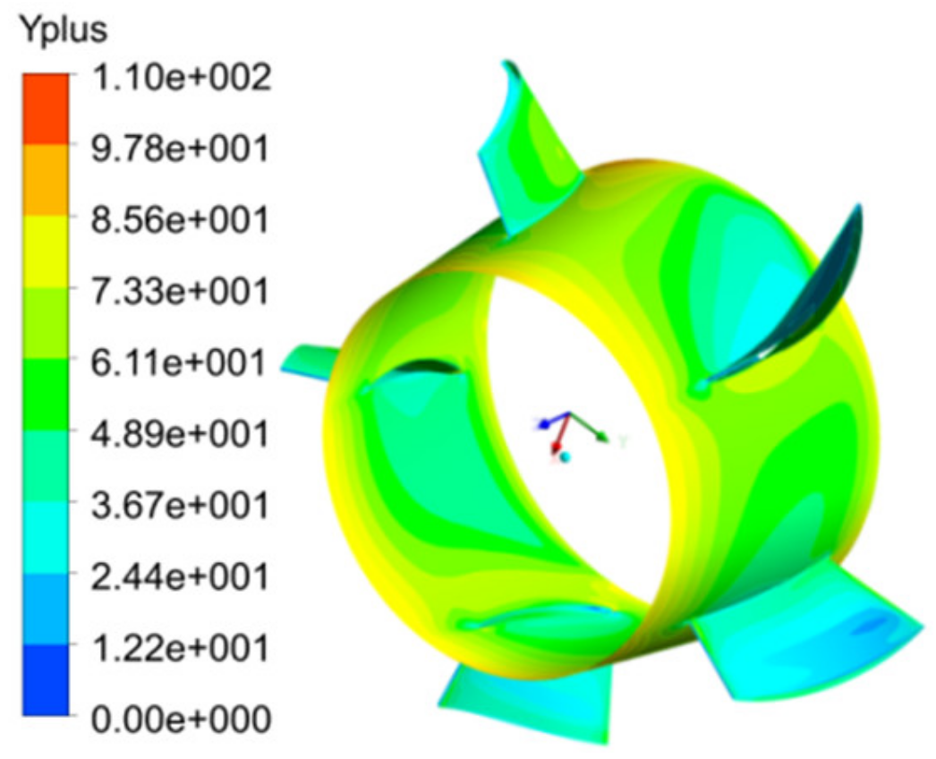
2.2. Mesh Generation

A hybrid mesh was employed during the mesh generating process. In terms of the intake duct, the impeller and the vane, they were meshed with the IGG software, and the hexahedral mesh took up the most. As shown in Figure 2, “H-O-H” type grids were applied to mesh the intake duct, the impeller, and the vane; a mesh refinement technique was used to capture the flow near the walls. The other zones in the computational domain of Figure 1 were meshed using the Gambit software, which mainly consisted of the tetrahedral mesh and the hexahedral mesh. During the meshing process, the partial refinement technique and the cooper method were united together to generate the high-quality mesh.

Since the near-wall treatment is important for the turbulence model, Figure 3 presents the Yplus distribution on the impeller and the vane, and the largest value of Yplus is lower than 110, which satisfies the basic standard of using the turbulence model (SST k-ω) [8].

2.3. Numerical Settings and Its Validation

2.3.1. Basic Governing Equations

When the underwater vehicle operates, there exists the inevitable cavitating flow into the high-speed water jet propulsion pump. In terms of the turbulent cavitating fluid, it could be defined as the uniform mixture flow comprised of the water and vapor [19]. To describe these complex flows, the governing equations for the unsteady Reynolds average Navier–Stokes method are given as:

$$\frac{\partial {\rho }_m}{\partial t}+\frac{\partial \left({\rho }_m{u}_j\right)}{\partial x_j}=0$$

(1)

$$\frac{\partial \left({\rho }_m{u}_i\right)}{\partial t}+\frac{\partial \left({\rho }_m{u}_i{u}_j\right)}{\partial x_j}=-\frac{\partial p}{\partial x_i}+\frac{\partial }{\partial x_j}\left[({\mu }_m+{\mu }_t)\left(\frac{\partial u_i}{\partial x_j}+\frac{\partial u_j}{\partial x_i}-\frac{2}{3}\frac{\partial u_k}{\partial x_k}{\delta }_{ij}\right)\right]$$

(2)

where $i=1,2,3, j=1,2,3, k=1,2,3$; $x_i,x_j,x_k$ are the Cartesian coordinate components; $u_i,u_j,u_k$ denote the velocity components; $p$ is the static pressure; ${\mu }_t,{\mu }_m$ are the turbulent viscosity and the mixture dynamic viscosity separately; ${\rho }_m$ is the mixture density. The mixture dynamic viscosity ${\mu }_m$ and the mixture density ${\rho }_m$ can be transformed as:

$${\rho }_m={\rho }_v{\alpha }_v+{\rho }_l\left(1-{\alpha }_v\right)$$

(3)

$${\mu }_m={\mu }_v{\alpha }_v+{\mu }_l\left(1-{\alpha }_v\right)$$

(4)

where the subscript $\nu$ and the subscript $l$ are the vapor phase and water phase.

The occurrence of cavitation is accompanied by the phase change of the thermodynamics and kinetics. To describe this converting mass transfer rates between the vapor and the liquid, the source terms m⁺ and m⁻ can be quantitatively described as:

$$m^{+}=F_{evap}\frac{3{\alpha }_{ncg}\left(1-{\alpha }_{\nu }\right){\rho }_{\nu }}{R_b}\sqrt{\frac{2}{3}\frac{Max\left(p_{\nu }-p,0\right)}{{\rho }_l}}$$

(5)

$$m^{+}=F_{cond}\frac{3{\alpha }_{\nu }{\rho }_{\nu }}{R_b}\sqrt{\frac{2}{3}\frac{Max\left(p_{\nu }-p,0\right)}{{\rho }_l}}$$

(6)

where ${\alpha }_{\nu }$ is the vapor volume fraction; the related variables are $F_{evap}=50$, $F_{cond}=0.01$, ${\alpha }_{ncg}=5\times {10}^{-4}$ and $R_b={10}^{-6}$. Based on the defined source terms m⁺ and m⁻, the Rayleigh–Plesset equation used to weigh a balanced relationship are further defined as follows:

$$\frac{\partial \left({\rho }_{\nu }{\alpha }_{\nu }\right)}{\partial t}+\frac{\partial }{\partial x_j}\left({\rho }_{\nu }{\alpha }_{\nu }{u}_j\right)=m^{+}-m^{-}$$

(7)

The above cavitating theory was primarily proposed by Schnerr and Sauer [20], which was embodied into the codes of the ANSYS-CFX solver. After some minor modifications, the cavitation model was improved to make it much more appropriate to simulate the jet pump [1,19].

2.3.2. Basic Governing Equations

To simulate the inner flow of the underwater cruising vehicle, an unsteady Reynolds-averaged Navier–Stokes simulation method for incompressible flow was adopted. Due to the Reynolds stress, the turbulence model needs to be imported to describe the stress. Regarding the turbulence model, the standard model and the SST model were often used [21]. As for these two kinds of turbulence models, they both were chosen to be validated. Moreover, through the comparative analysis, a much more appropriate turbulence model was chosen next.

As mentioned previously, the simulation process was implemented in the CFX solver. The basic settings of the boundary conditions had already been illustrated in Part 2.1. The simulation process consisted of three stages: the first stage was the steady simulation without cavitating; the second stage was the unsteady simulation without cavitating; the third stage was the unsteady simulation with the cavitation. Along with the second-order unwind discretization for the convection term, the convergence indicator for these three different stages were the convergence indicator for the steady simulation was 10⁻⁵; during the unsteady simulation stage, the single time step was 0.47619 × 10⁻⁵ s, and the physical iteration of steps at each time step was 20 with a single step convergence of 10⁻⁷.

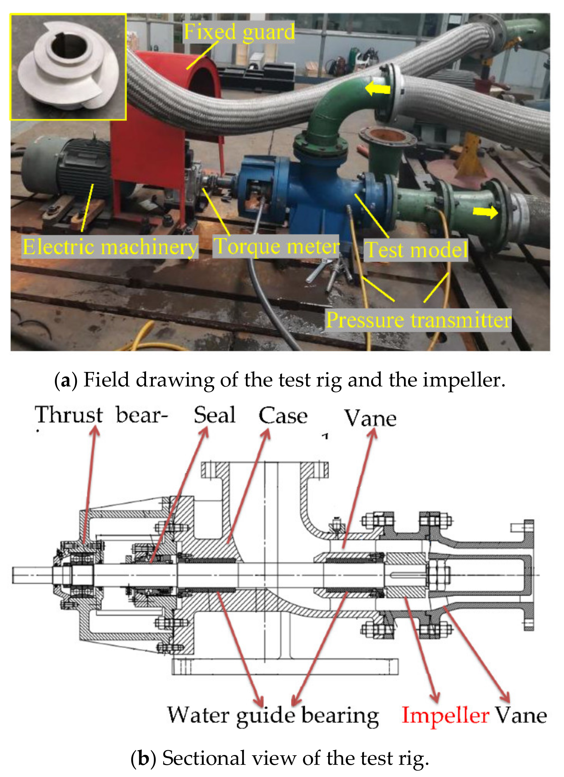
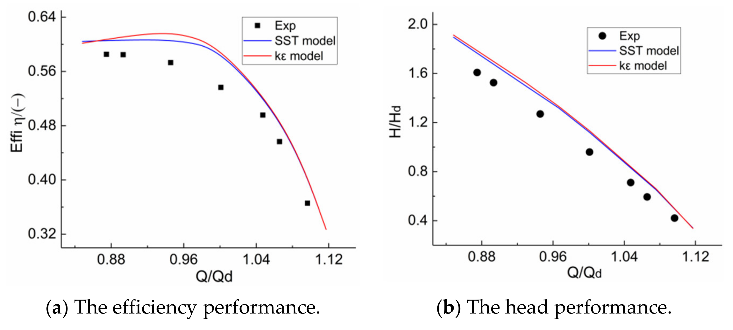
2.3.3. Validation of the Numerical Approach via the Speed Reduction Experiment

To explore the appropriate turbulence model and validate the feasibility of the numerical approach, the core hydraulic components comprised of the impeller and the vane are taken as the test model. Based on the determined boundary conditions illustrated in Part 2.1, the test rig was set up as shown in Figure 4. As shown in Figure 4b, the test section was from the impeller inlet to the vane outlet. In correspondence to the identified test section, the simulating zone was settled down. In terms of the simulating zone, the numerical simulation was then implemented with the illustrated approach.

The same as the experimental conditions, the hydraulic models consisted of an impeller and a vane simulated with the numerical settings illustrated above. The results are presented in Figure 5. In the figure, through the comparative analysis of the standard model and the SST model, it was inferred that minor errors existed between these two models. Additionally, through the comparative analysis of the simulating results of the experimental results, it was found that they had the same increasing and decreasing trends. In addition, we found that the simulating performance obtained from SST was a little lower than the model, which was much more close to the experimental result. Thus, the SST turbulence model was adopted in the simulating process of this study. Since the design condition was the main study focus, the head and the efficiency at the design condition were less than 2.6%, 2.1% separately, which satisfies with the permitted standard [11,14].

3. Results and Discussions

3.1. Effects of the Cruising Speed on the Overall Performances

As mentioned in the title of the article, the investigation of the cruising speed on the underwater vehicle’s performance was the main focus of this study. As a result, with the other influencing factors, such as the matching components, the tip clearance size, etc., unchanged, the cruising speed was the main key factor to be carefully considered and explored. The quantitative performances of the underwater vehicle and the pump system consisted of the efficiency $\eta$, the head $H$, the thrust $T_r$, and the power $P_c$, which could be settled down with the following formulas:

$$H=\frac{p_{out}-p_{in}}{\rho g}$$

(8)

$$\eta =\frac{\rho gH}{\tau \omega }$$

(9)

$$T_r=Q_m\left(V_{out}-U\right)$$

(10)

$$P_c=\tau \omega$$

(11)

where $P_{in},P_{out}$ are the total pressure at the inlet and outlet of the pump; $\omega$ is the rotating speed; $V_{out}$ is the velocity of the water from the water jet pump; $\tau$ represents the torque of the impeller; $Q_m$ is the massflow passing through the water jet pump.

Figure 6 shows the effects of the cruising speed on the overall performance of the underwater vehicle. In Figure 6a, as the cruising speed of the underwater vehicle improves, the passing massflow of the pump system had the same trend, whose ranges fall into 256–295 kg/s. The simulated pump performances are presented in Figure 6b, which implies that the calculated design head was about 134 m, and the corresponding efficiency was 69.2%. Additionally, Figure 6c denotes that the cruising velocity had an obvious effect on the thrust and power of the whole underwater vehicle, and the design thrust for the pump system was about 7960 N with an energy consumption of 5400 W.

To reveal the effects of cursing speed on the steady performances, three scatter kinds of cruising speeds comprised of 0.5 Ud, 1.0 Ud, 1.7 Ud were further analyzed. To make a supportive analysis of the effects of the cruising speed, Figure 7 shows the distribution of streamline and pressure on the underwater vehicle. As shown in the figure, we found that the pressure remained stable on the navigation body and then increased gradually from the pump inlet to the pump outlet. In addition, through the comparative analysis of the pressure on the hydraulic components, we found that the impeller zone had the highest pressure, which was mainly caused by the input work. When the cursing speed decreased, it led to an obvious pressure decline in the pump system. Then, by comparison of the streamlines on the navigation body, they had similar distributing characteristics under different cruising speeds. However, in terms of the pressure, the larger the cruising speed was, the higher the pressure around the pump inlet was.

3.2. Steady Evaluation of the Effects of the Cruising Speed on the Performances Based on the Energy Loss Theory

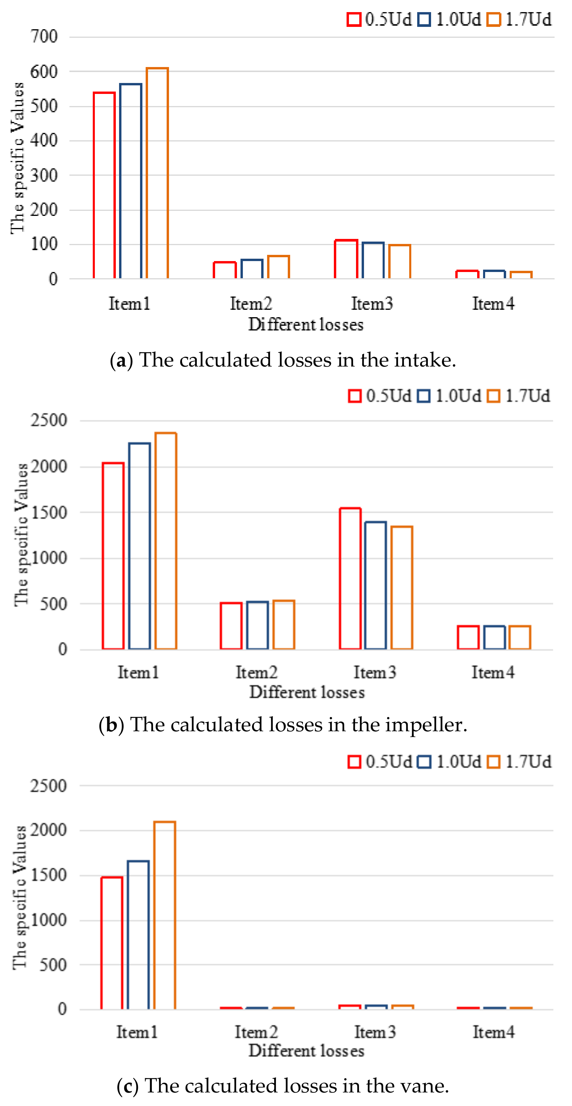
3.2.1. Study of the Energy Loss in the Pump System under Different Cruising Speeds

Figure 8 presents the distribution of the streamline at the 50% blade high location, which illustrates that the high loss areas tended to appear at the leading edge of the intake, the trailing edge of the impeller, and the suction surface of the vane. However, by comparison of the flow field represented with the streamlines, it was found that they have similar distributing characteristics.

To better understand the relationship between the flow patterns and the losses in the underwater cruising vehicle, a local loss analysis approach [21] established on the energy balance equation was conducted. The energy balance equation was introduced to clarify the mechanism of the energy loss owing to the complex flow and provide an understanding of the interaction between the energy loss and the flow features. Here, the energy balance equation was mainly imported to clarify the flow mechanism of the energy losses caused by the underwater vehicle’s cruising speed and provided a better understanding of the inner flow characteristics and the energy losses.

For the incompressible turbulent flow, the energy equation can be expressed as follows [8]:

$$\frac{\partial }{\partial t}\left(\frac{1}{2}\rho {\overline{u}}^2\right)+\frac{\partial \left[{\overline{u}}_j\left(\frac{1}{2}\rho {\overline{u}}^2+\overline{p}+\rho gz\right)\right]}{\partial x_j}=\frac{\partial \left(-{\overline{u}}_i\overline{\rho u_i^{\prime }{u}_j^{\prime }}\right)}{\partial x_j}+\mu \frac{\partial \left({\overline{u}}_i\overline{D_{ij}}\right)}{\partial x_j}-\left(-\overline{\rho u_i^{\prime }{u}_j^{\prime }}\right)\frac{\partial {\overline{u}}_i}{\partial x_j}-\mu \overline{D_{ij}}\frac{\partial {\overline{u}}_i}{\partial x_j}$$

(12)

where $D_{ij}$ can be represented by the following formula:

$$D_{ij}=\frac{\partial u_i}{\partial x_j}+\frac{\partial u_j}{\partial x_i}$$

(13)

Since the turbulent flow is highly time-dependent, it is not necessary to discuss the contribution of the variation of the kinetic energy. Accordingly, in terms of the energy balance equation of Equation (12), it can be integrated over the total volume and transformed as follows:

$$P_L= -\frac{{\displaystyle \underset{V}{\iiint }\frac{\partial (-\overline{u_i}\overline{\rho {u_i}^{\prime }{u_j}^{\prime }})}{\partial x_j}}dV}{\mathrm{Item}1}-\frac{{\displaystyle \underset{V}{\iiint }\mu }-\frac{\partial (\overline{u_i}\overline{D_{ij}})}{\partial x_j}dV}{\mathrm{Item}2}+\frac{{\displaystyle \underset{V}{\iiint }(-\overline{\rho {u_i}^{\prime }{u_j}^{\prime }}})\frac{\partial \overline{u_i}}{\partial x_j}dV}{\mathrm{Item}3}+\frac{{\displaystyle \underset{V}{\iiint }\mu }\overline{D_{ij}}\frac{\partial \overline{u_i}}{\partial x_j}dV}{\mathrm{Item}4}$$

(14)

and the Reynolds stress Equation (14) can be further calculated with the following formula according to the Boussinesq approximation assumption:

$$-\overline{\rho u_i^{\prime }{u}_j^{\prime }}={\mu }_t\left(\frac{\partial \overline{u_j}}{\partial x_i}+\frac{\partial \overline{u_i}}{\partial x_j}\right)-\frac{2}{3}{\delta }_{ij}\rho k$$

(15)

In Equation (8), item 1 and item 2 denote the diffusion of the kinetic energy caused by the diffusion of the kinetic energy from the high-speed external flow to the low-speed separation flow by means of the Reynolds stress and the viscous stress [22,23]; item 3 is the turbulent kinetic energy production, which is from the transmission of the kinetic energy to the turbulent kinetic energy; item 4 is the viscous dissipation of mean kinetic energy, which is from the kinetic energy dissipated by the effect of the viscous stress.

In terms of the three kinds of cruising speeds (0.5 Ud, 1.0 Ud, 1.7 Ud) in Figure 6c, their corresponding simulating results are processed with the energy balance equation in Equation (8), whose results are given in Figure 9. Through comparative of the different losses listed in the figure, it was found that the kinetic energy diffusion from the Reynolds stress (item 1) and viscous stress (item 2) presented an increasing trend along with the increase the cruising speed, while the turbulent kinetic energy production (item 3) and the viscous dissipation (item 4) appear a completely opposite trend. To support this phenomenon, Figure 6 shows that the increasing cruising speed resulted in a rise of the massflow into the water jet pump, which enlarged the separation flow from the high-speed external flow to the low-speed inner flow, and the losses of item 1 and item 2 were also enlarged.

Moreover, by comparing the losses in different hydraulic components of Figure 9, it can be seen that the losses in the rotating impeller were much larger than the losses in the static intake and vane. Moreover, as for the static components, apart from the kinetic energy diffusion from the Reynolds stress (item 1), the other three kinds of losses (item 1, 2 and 3) in the vane were lower than the intake. In Figure 9, it was found that the kinetic energy diffusion from the Reynolds stress (item1) and the turbulent kinetic energy production (item 3) were much larger than the other two kinds of losses (item 2 and item 4), especially the viscous dissipation could be ignored due to the existence of the high Reynolds number of the working flow. The effects of the cruising speed on the key losses consisted of item 1 and item 3 can be further clarified.

As mentioned above, the kinetic energy diffusion caused by Reynolds stress (item 1) and the turbulence kinetic energy production (item 3) are the main losses for the hydraulic components of the water jet pump system. Accordingly, their circumferential averaged distributing contours at the blade middle height location are extracted and shown in Figure 10, Figure 11 and Figure 12. As clearly seen in the figure, the higher the cruising speed was, the higher the kinetic energy diffusion by Reynolds stress (item 1) and the lower the turbulence kinetic energy production was, which satisfies the overall distribution law of the calculated losses in Figure 9.

Figure 8 has already shown the overall distribution of the streamline for the pump system. In the figure, there are no obvious large-scale distortions for the flow field, which replies the advancement of the newly developed hydraulic model. In addition, as marked with the black circle in the figure, it was found the vortexes were much more likely to appear at the leading edge of the intake blade, the trailing edge of the impeller blade and the pressure side of the vane blade, which agrees with the distributing law of the extracted loss contours of Figure 10, Figure 11 and Figure 12. Overall, via the energy loss analysis, the losses were clarified and understood according to the hydraulic components and the loss types.

3.2.2. Statistical Analysis of the Inner Flow Characteristic of Key Hydraulic Component with the Highest Energy Losses

• Quantitative extraction of the typical factors

Among the extracted losses of the hydraulic components shown in Figure 9, the rotating impeller had the highest losses. Therefore, revealing the related mechanism is crucial. In addition, the impeller was chosen as the study focus in this part since there was inevitable tip clearance between the blade tip and the shroud in Figure 1, which generated the tip clearance flow and greatly influenced the performance of the underwater vehicle and water jet pump.

Based on the energy loss analysis result, this section tries to clarify the mechanism of tip clearance flow under different cruising speeds. According to related studies [23], it has been reported that the blade tip load and the scraping effect from the shroud are the main factors to determine the leakage flow. Moreover, these key factors were quantitatively extracted and analyzed. As presented in Figure 13, the blade tip clearance was divided into 20 small zones. In terms of these small zones, the pass leakage flow can be represented with the leakage intensity $Q_l$, which can be calculated with the following formula:

$$Q_l=\frac{{\displaystyle \int {\rho }_{l}w·n}d{A}_l}{{\displaystyle \int d{A}_l}}$$

(16)

where ${\rho }_l$ is the density of the fluid medium; $A_l$ is the divided zone’s marked section in Figure 13; $w$ is the relative velocity passing through the divided zone; $n$ is the normal vector of the divided zone.

Moreover, the blade tip load $\Delta P_l$ can be settled down with the following formula:

$$\Delta P_l=P_{ps}-P_{ss}$$

(17)

where $P_{ps},P_{ss}$ reply the static pressure on the pressure and suction side at the blade tip.

With the application of Equations (16) and (17), the distribution of the calculated leakage intensity and the blade tip load for the 20 divided zones along the streamline are given in Figure 14 and Figure 15. In the figure, it can be seen that there was a significant drop in the leakage intensity. In contrast, with the increase of the cruising speed, the streamline location of the lowest point became smaller, while the Y value of the lowest point became larger. To explain this phenomenon, Figure 15 shows the distribution of the blade load. Through the comparative analysis of these two figures, we found that they had almost the same increasing and decreasing trends. As a result, it was demonstrated that the changing trend of the blade load results in the distributing characteristics of the leakage intensity; namely, the tip blade load was the main factor to determine the leakage intensity. Nevertheless, at the 0.2–0.6 blade streamline location, the leakage intensity had a completely opposite trend in relative to the blade load, therefore, there is a reason to believe that another factor acts on the leakage flow.

As shown in the lower right corner of Figure 16, it was found that the existence of the static casing had an obvious promoting effect on the tip clearance leakage flow. In addition, so as to quantitatively describe the effect of the scraping effect from the static casing, the scraping pressure can be identified according to a similar study on a radial inflow turbine [24]:

$$P_s=0.5\rho u^2{\cos }^2\beta$$

(18)

where $u$ is the circumferential velocity; $\beta$ is the install angle at the blade tip.

Based on Equation (18) and the previous known install angle, the calculated scraping pressure is shown in Figure 16. In the figure, around the 0.75 blades streamline location, there was a peak value for the scraping pressure, which made up for the sharp dropping trend of the pressure load in Figure 15, and the superimposed effects resulting in the distributing trend of the leakage intensity in Figure 14.

• Quantitative analysis with the statistical method

The main factors determining the blade tip clearance leakage flow were previously extracted, and the overall distributing law was clarified. To make a further analysis about the influencing factors related to the leakage flow, the partial least-squares (PLS) analysis method was adopted. With the integration of the advantages of the canonical correlation analysis method, the principal component analysis method and multiple linear regression analysis methods, the PLS method cannot only consider the linear and nonlinear relationship between dependent variables and independent variables but also can avoid potential threatens, such as non-normal distributing problem about data and uncertainty problem of data structure.

By setting the pressure load $\Delta P_l$ and the scraping pressure $P_s$ as the dependent variable, the leakage intensity $Q_l$ can be represented and analyzed with the regression equation as follows:

$$Q_l=K(a_1{P}_s+a_2\Delta P_l+a_3{P}_s^2+a_4\Delta P_l^2+a_5{P}_s^3+a_6\Delta P_l^3+a_7{P}_s\Delta P_l)$$

(19)

where $a_i(i=1,2,3,4,5)$ are the coefficients determining the regression equation. Based on Equation (14), the main steps to implement the PLS analysis are as follows:

Step 1. Standardize the independent variable $Y$ (the leakage intensity $Q_l$) and the dependent variable $X$ (the scraping pressure $P_s$ and the pressure load $\Delta P_l$), and mark them as $F_0$ and $E_0$ separately.

Step 2. Extract the first pair of the principal component $t_1$ ($t_1=E_0{w}_1$, $\left|\right|w_1\left|\right|=1$) and $u_1$ ($u_1=F_0{c}_1$, $\left|\right|c_1\left|\right|=1$) from the standardized $E_0$ and $F_0$, which should obey the following standard as:

$$\underset{u_1,c_1}{\max }<E_0{w}_1,F_0{c}_1> st.\left\{\begin{array}{l}{w}_1^{\prime }{w}_1=1\\ c_1^{\prime }{c}_1=1\end{array}\right.$$

(20)

Step 3. After the extraction of $t_1$ and $u_1$, carry out the regression analysis between $X,Y$ and $t_1$, and then, the coefficients can be settled down after eliminating the intermediate variable $t_1$.

Step 4. Check the feasibility of the analysis result with the following formula:

$$Q_h^2=1-\frac{PRES{S}_h}{S{S}_{(h-1)}}$$

(21)

where $Q_h^2$ is the cross-validation index; $PRES{S}_h$ is the sum of the predicting error square; $S{S}_{(h-1)}$ is the sum of the error square. It is required that $Q_h^2$ should be larger than 0.0975.

Step 5. Calculate and output the variable projection importance index ($VI{P}_i$) to judge the influence of the dependent variable $X$ on the independent variable $Y$:

$$VI{P}_i=\sqrt{\frac{P}{Rd(Y;t_1,\wedge ,t_m)}{\displaystyle \sum _{h=1}^{m}Rd\left(Y;t_h\right)w_{hi}^2}}$$

(22)

where $P$ is the number of the variables; $m$ are the pairs of the principal components; $w_{hi}$ is the i^th component of $w_h$; $Rd(Y;t_1,\wedge ,t_m)$ represents the cumulative explanatory power between $t_1,\cdots ,t_h$ and $Y$. Usually, the variable $VI{P}_i$ can be taken as the indicator to weigh the importance of the influence factor. As for the effects of the dependent variables on the independent variable, $VI{P}_i>1$ can be taken as the important level, $0.5<VI{P}_i<1$ can be taken as the less important level, and $VI{P}_i<0.5$ can be taken as the unimportant level.

Based on the above analysis principle, the regression coefficients are settled down and presented in

Table 1. Calculated coefficients under different cruising speeds.

	ΔPl	Ps	ΔPl2	Ps2	ΔPl3	Ps3	PsΔPl	Constant
0.5Ud_blade1	4.61121	0.24138	−1.33613	0.33142	−0.55116	−0.105519	2.55449	2.90862
0.5Ud_blade2	0.29420	−0.070853	−0.288536	0.17669	0.302952	−0.099124	0.058782	2.97665
1.0Ud_blade1	0.29236	−0.24780	−0.117941	0.16114	0.241065	−0.217961	0.105077	2.9786
1.0Ud_blade2	0.96155	−0.070169	−0.144005	0.40447	−0.27758	−0.082514	0.329794	2.98942
1.7Ud_blade1	0.44893	−0.295156	−0.134373	0.93065	−0.25488	−0.254882	−0.033486	2.48699
1.7Ud_blade2	0.33432	−0.357459	−0.080798	0.69957	−0.33142	−0.043504	−0.143451	2.62507

, whose corresponding fitted curves are presented in Figure 17. In the figure, the fitted curve with PLS can be well in accordance with the original result obtained with CFD, which demonstrates the feasibility of the analysis result. Namely, it can be considered that the regression model from the PLS analysis method can better predict the leakage intensity and can clearly obtain the quantitative relationship between the blade load, the scraping pressure, and the leakage strength.

Along with the fitting process, the variable projection importance indexes ($VI{P}_i$) to judge the influence of the dependent variable (the tip load and the scraping pressure) on the independent variable (the leakage intensity) are calculated at the same time. The calculated results are shown in Figure 18. In the figure, it was found that the increase of the cruising speed led to the decrease of the tip load’s $VI{P}_i$ value, which means that the influence from the tip load comes to be weaker when the cruising speed becomes larger. Nevertheless, the scraping pressure’s $VI{P}_i$ value rises with the increasing cruising speed, which means that the effect from the scraping pressure tends to be larger.

As presented in the energy loss analysis result of Figure 9b, it was found that the diffusion of the kinetic energy from the high-speed external flow to the low-speed separation flow by means the viscous stress (item 2) increased with increasing cruising speed. Actually, the scraping pressure is generated from the viscous stress of the static shroud. As presented in Figure 9b and Figure 18, both the scraping pressure and the kinetic diffusion from the viscous stress increased with the enlargement of the cruising speed.

3.3. Unsteady Evaluation of the Effects of the Cruising Speed on the Hydraulic Components’ Performance

3.3.1. Pressure Pulsation Analysis

After the execution of the steady performance analysis, it can be found out that the cruising speed has an obvious effect on the underwater vehicle and the water jet pump performance. Based on the steady result, the unsteady performances influenced by the cruising speed are to be simulated. The basic settlement for the unsteady simulation process is presented in Part 2.3. Under one single time step, the impeller’s rotating angle is 0.5°, and the iterative step is set to be 20. After calculating 12 rotating cycles, the unsteady data from the 13–14th circle are to be provided for further analysis.

The pressure pulsation is not useful for the concealment of the underwater vehicle. In addition, too large pressure pulsation caused damage to the hydraulic components. As a result, it is of great importance to evaluate the effects of the cruising speed on the pressure pulsation. Figure 19 shows the information of the monitoring points on the middle height of the blade surface, namely, PI1–PI4 are the points in the intake, PM1–PM4 are the points in the impeller, and PV1–PV4 and are the points in the vane.

The non-dimensional pressure coefficient can be settled down with the following formula:

$$C_p=\frac{P_i-\overline{P}}{0.5\rho u_2^2}$$

(23)

where $P_i$ is the transient pressure; $\overline{P}$ is the averaged pressure at the inlet of the impeller.

As for the 12 monitoring points marked in Figure 19, the corresponding calculated pressure pulsations are shown in Figure 20. On the whole, influenced by the rotating impeller, the amplitudes of the monitoring points (P_I1, P_I2, P_I3) in the intake increase along the streamline, while the amplitudes of the monitoring points (P_V1, P_V2, P_V3) in the vane take a decreasing trend. In addition, by comparison of the scatter three monitoring points in the rotating impeller, the amplitude at the P_M1 point is larger than the other two monitoring points (P_M2, P_M3) obviously, which implies that the stator-rotor intersections between the static intake vane and the rotating impeller cannot be ignored.

To make an intuitive presentation of the effects of the cruising speed on the pressure pulsations. The unsteady pressure fluctuation intensity can be herein defined as [25]:

$$\overline{p}=\frac{1}{M}{\displaystyle \sum _{n=1}^N{p}_i\left(x,y,z,\frac{n}{360}T\right)}$$

(24)

$$p_{sdv}=\sqrt{\frac{1}{M-1}{{\displaystyle \sum _{n=1}^N\left[p_i\left(x,y,z,\frac{n}{360}T\right)-\overline{p}\right]}}^2}$$

(25)

where is $p_i\left(x,y,z,\frac{n}{360}T\right)$ the local pressure on each grid node; $T$ is the periodic time; $M$ represents the number of the output files at the defined periodic time.

With the application of Equations (24) and (25), Figure 21 shows the calculated pressure fluctuation intensities around the underwater vehicle. As clearly seen from the figure, it can be seen that the maximum pressure pulsation zone tends to appear at the outlet of the pump system. In addition, the larger the cruising speed is, the much larger the pressure pulsation was.

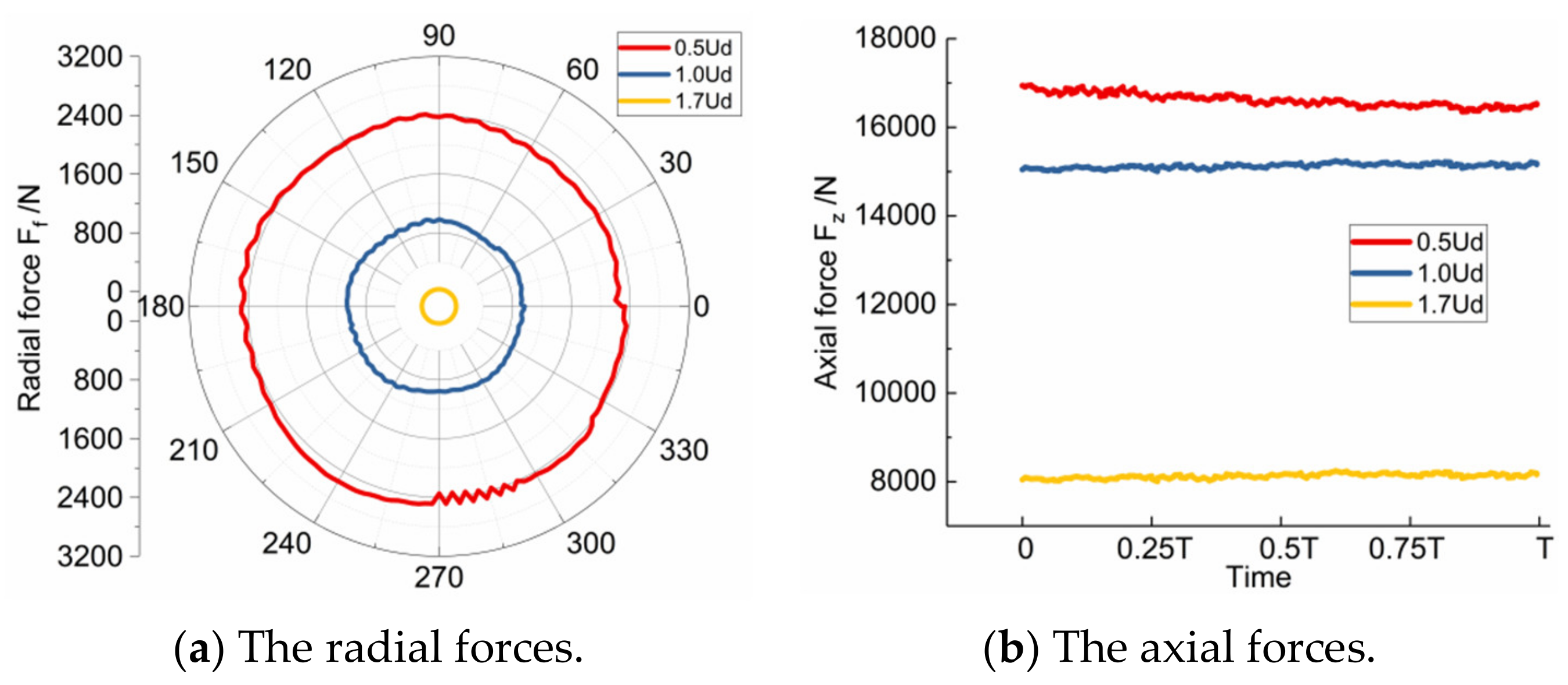
3.3.2. Radial and Axial Force Analysis

In terms of the working process for the pump system, the unsteady forces comprised of the radial forces and the axial forces from the rotating impeller have a direct influence on the operating stability of the underwater vehicle. The radial force is crucial for the circumferential balance, and the axial force is the key factor to guarantee the safe working process of the bearing. The calculating formulas for the radial force and the axial force are as follows:

$$F_r=\sqrt{{\left({\displaystyle \int p_{x,t}d{A}_{blade}+{\displaystyle \int p_{x,t}d{A}_{hub}}}\right)}^2+{\left({\displaystyle \int p_{y,t}d{A}_{blade}+{\displaystyle \int p_{y,t}d{A}_{hub}}}\right)}^2}$$

(26)

$$F_z={\displaystyle \int p_{x,t}d{A}_{blade}+{\displaystyle \int p_{x,t}d{A}_{hub}}}$$

(27)

where $A_{blade}$ is the impeller blade surface; $A_{hub}$ is the impeller hub surface; $p_{x,t},p_{y,t},p_{z,t}$ are the instantaneous pressure at different directions.

After the execution of Equations (21) and (22), Figure 22 gives the calculated unsteady forces. As shown in the figure, the 0.5 Ud cruising speed had a radial force of about 2000 N and an axial force of about 17,000 N, the 1.0 Ud cruising speed had a radial force of about 800 N and an axial force of about 15,000 N, and the 1.7 Ud cruising speed had a radial force of about 60 N and an axial force of about 8000 N. Through comparative analysis, it was found that the improvement of the cursing speed led to the decrease of the unsteady forces.

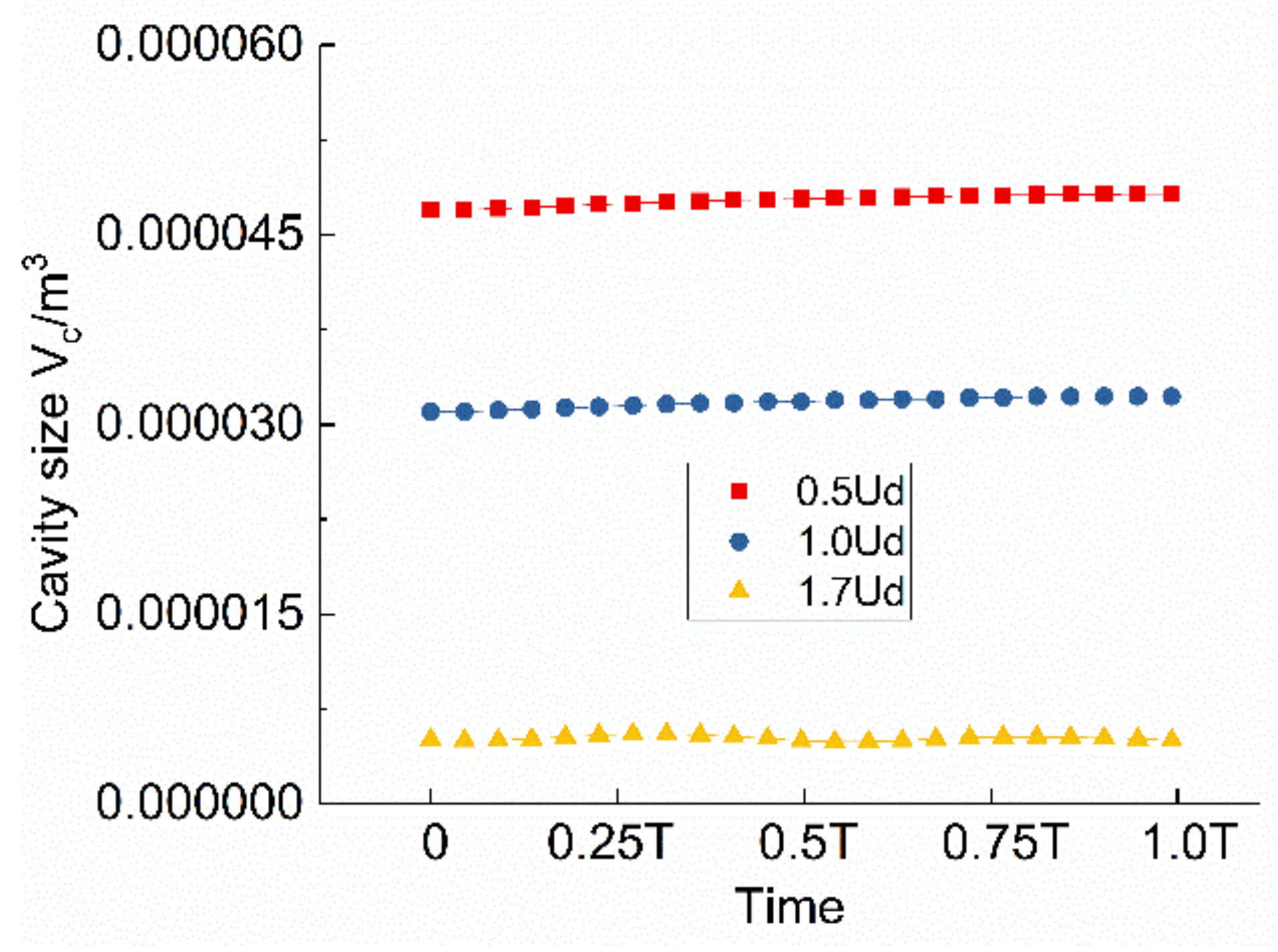
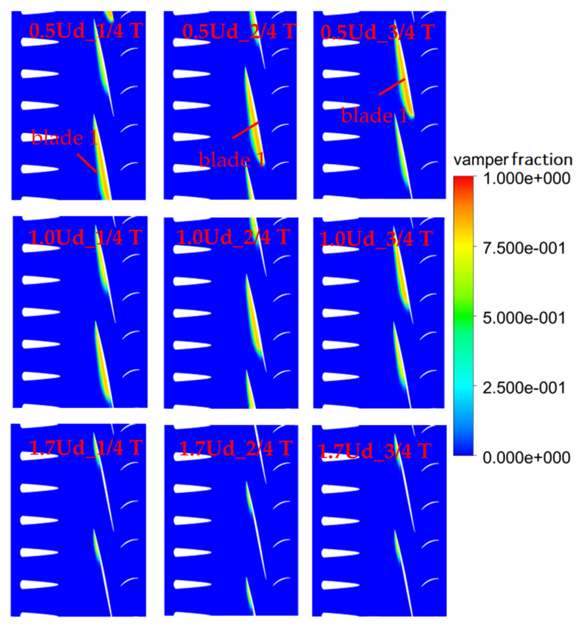
3.3.3. Cavitating Analysis

Since the water jet pump of this study belongs to the high-speed pump, which exists inevitable cavitating phenomenon, accompanied by the phase change of the thermodynamics and kinetics, the characteristics of cavitation influenced by the cruising speed are clarified in this section.

Aiming at the steady simulating results, Figure 23 shows the distribution of the cavity cloudy (0.05% vapor mass fraction). In the figure, of all the hydraulic components, the cavity cloudy just appears at the pressure side of the rotating impeller zone. Moreover, when the cruising speed increases, the cavity’s cloudy size becomes smaller.

To quantitatively describe the effects of the cruising speed on the volume of the cavitating cloudy, the transient cavity size $V_C$ can be adopted and defined as follows:

$$V_C={\displaystyle \int {\alpha }_{\nu }dV}$$

(28)

where $V$ is the volume of the computational domain.

Aiming at the unsteady simulating results changing with time, the corresponding calculated cavity cloudy sizes under different cruising speeds are presented in Figure 24. As seen from the figure, it is easily known that the cloudy cavity size under the 0.5 Ud, 1.0 Ud and 1.7 Ud cruising speed are about 4.5 × 10⁻⁵ m³, 3.1 × 10⁻⁵ m³, and 5.0 × 10⁻⁶ m³ separately. The quantitative results reply that the cavity cloudy size becomes smaller with the increasing cruising speed, which agrees with the extracted cavity cloudy distribution in Figure 22. Moreover, by observing the calculated cavity cloudy changing with time, it can be found out that the cloudy cavity size remains rather stable.

Further, for a more intuitive observation of the cavitating phenomenon, Figure 25 gives the distribution of the vapor fraction at the 90% blade height. In the figure, it can be seen that the cavitating phenomenon appears at the trailing edge first, and then it develops along the pressure side of the blade, which quite agrees with the extracted 3-D cavity cloudy in Figure 23.

4. Conclusions

By taking a newly developed high-speed water jet pump as the study object, the corresponding underwater vehicle’s operating characteristics influenced by the cruising speed were clarified. The following conclusions were obtained:

(1)

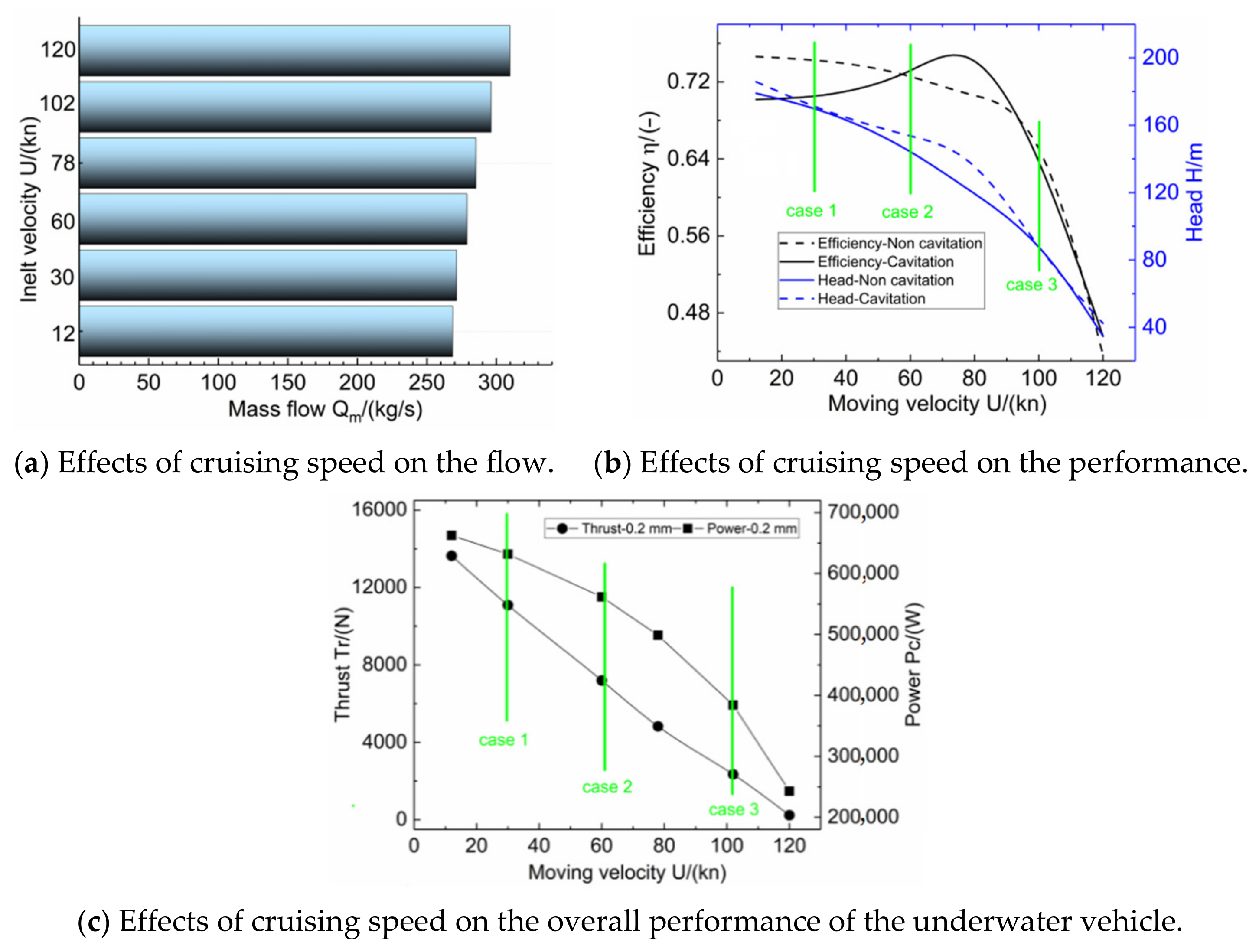
The overall performances influenced by the cruising speed were clarified. As the cruising speed of the underwater vehicle improved, the passing massflow into the pump system had the same increasing trend, while the performances comprised of the power, the thrust, the head, and efficiency decrease;

(2)

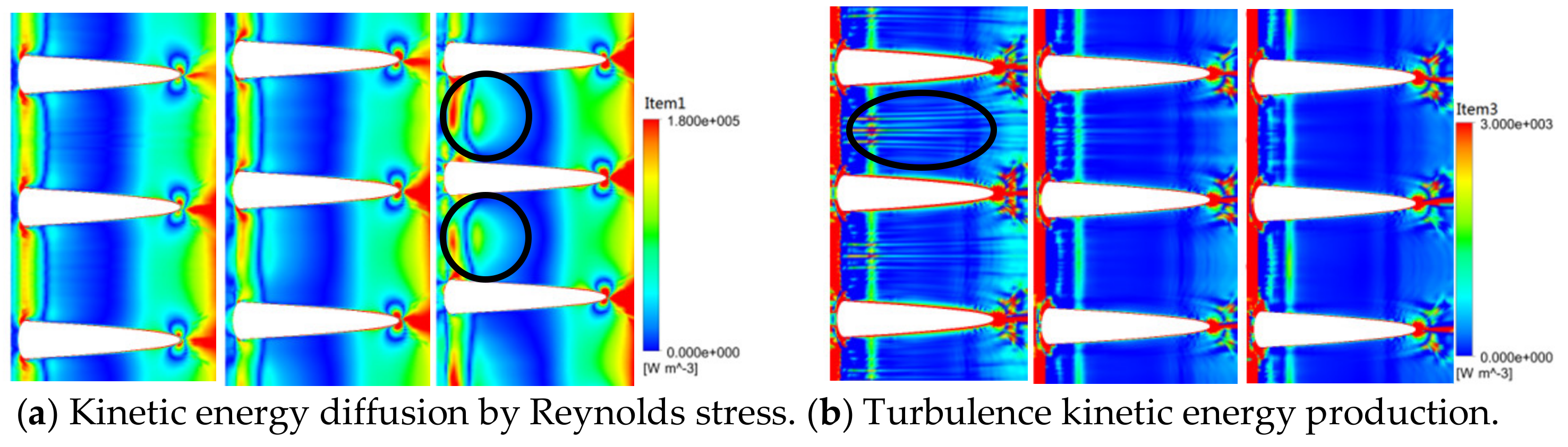
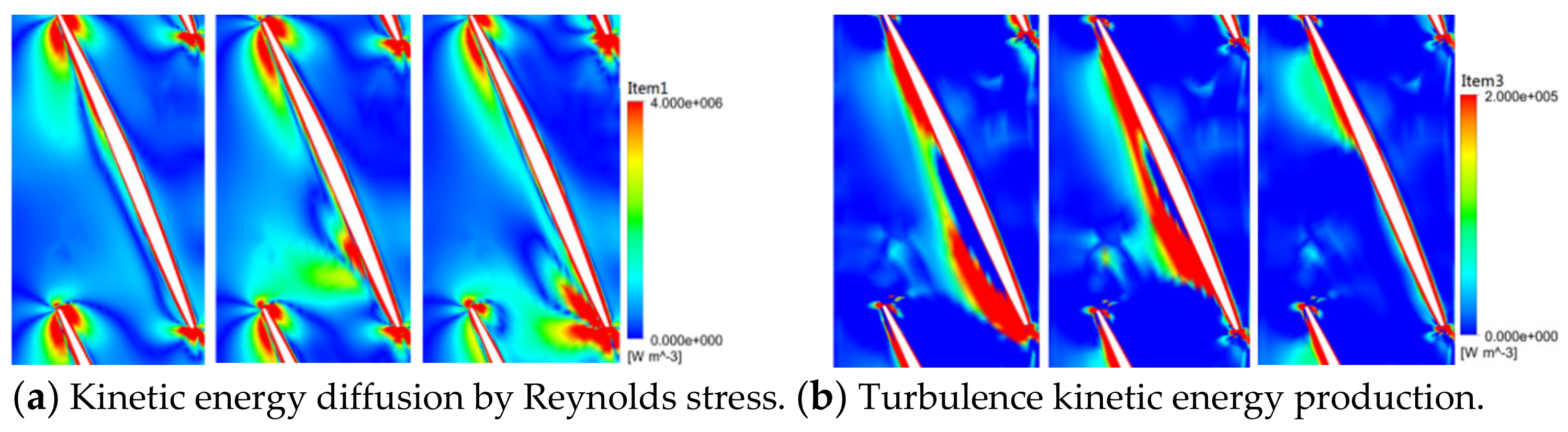
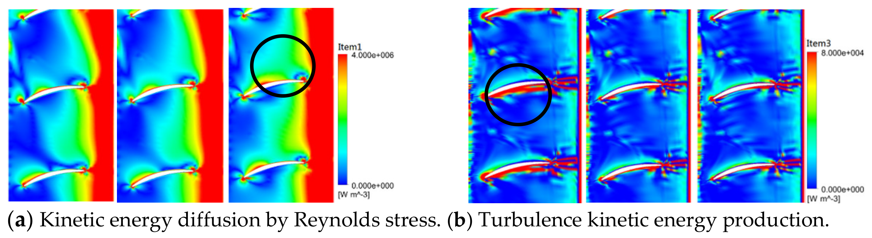
Established on the energy balance equation, the energy losses influenced by the underwater vehicle’s cruising speed were investigated. The kinetic energy diffusion from the Reynolds stress (item 1) and viscous stress (item 2) presented an increasing trend along with the increase in the cruising speed, while the turbulent kinetic energy production (item 3) and the viscous dissipation (item 4) showed a completely opposite trend. Item 1 and item 3 were the main losses in the water jet pump, followed by items 2 and 4. In addition, of all the hydraulic components, the rotating impeller zone had the highest losses;

(3)

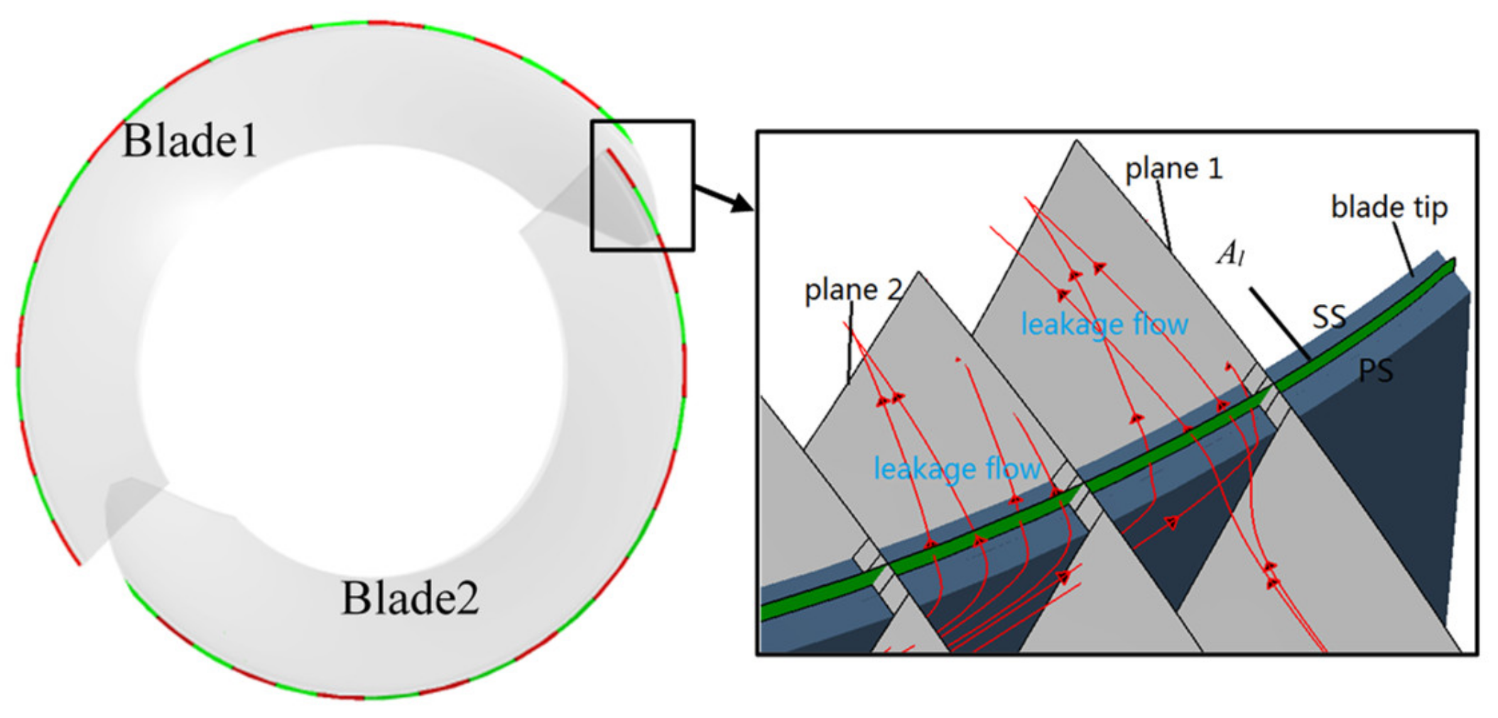
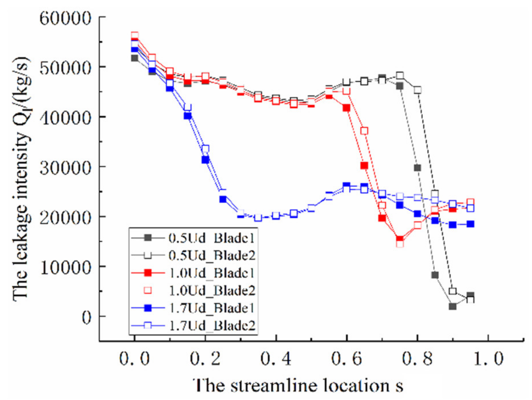
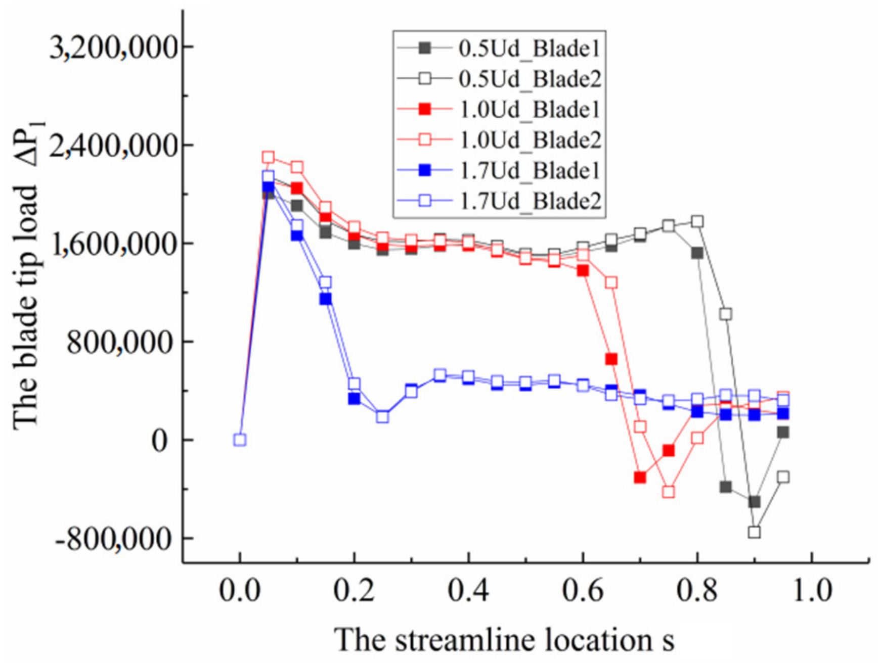
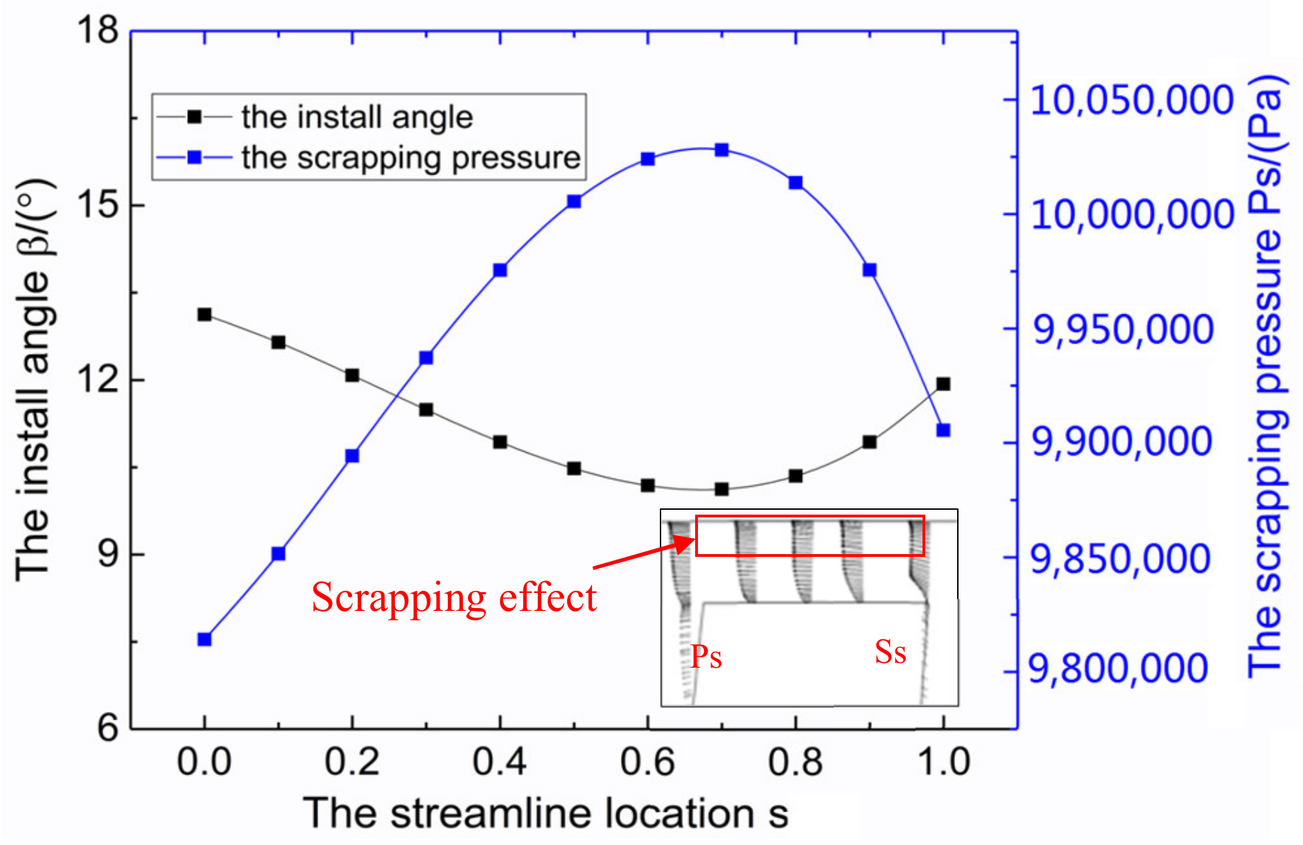
Based on the statistical analysis with the PSL method, the leakage flow’s characteristic of the rotating impeller with the highest energy losses was illustrated. First, the main factors determining the blade tip clearance leakage flow were previously extracted, and the overall distributing law was clarified. Then, the quantitative regression formulas were defined, and at the same time, it was demonstrated that the influence from the tip load comes to be weaker when the cruising speed became larger, while the effect from the scraping pressure tended to be larger.

(4)

After the execution of the unsteady analysis, the pressure pulsations, the unsteady forces, and the cavitation influence by the cruising speed were introduced. When the cruising speed increased, the pressure pulsation became larger, while the radial force, the axial force, and the cloudy cavity size became smaller.

References

1. Pan, G.; Lu, L.; Sahoo, P.K. Numerical simulation of unsteady cavitating flows of pumpjet propulsor. Ships Offshore Struct. 2015, 11, 1–11. [Google Scholar] [CrossRef]
2. Dai, C.; Zhang, Y.; Pan, Q.; Dong, L.; Liu, H. Study on vibration characteristics of marine centrifugal pump unit excited by different excitation sources. J. Mar. Sci. Eng. 2021, 9, 274. [Google Scholar] [CrossRef]
3. Park, W.-G.; Yun, H.S.; Chun, H.H.; Kim, M.C. Numerical flow simulation of flush type intake duct of waterjet. Ocean Eng. 2005, 32, 2107–2120. [Google Scholar] [CrossRef]
4. Jiao, W.; Cheng, L.; Zhang, D.; Zhang, B.; Su, Y.; Wang, C. Optimal design of inlet passage for waterjet propulsion system based on flow and geometric parameters. Adv. Mater. Sci. Eng. 2019, 2019, 2320981. [Google Scholar] [CrossRef] [Green Version]
5. Bulten, N.; Esch, B.V. Review of thrust prediction method based on momentum balance for ducted propellers and waterjets. In Proceedings of the ASME 2005 Fluids Engineering Division Summer Meeting, Houston, TX, USA, 19–23 June 2005. [Google Scholar]
6. Keegan, D.; Martin, D. Use of RANS for waterjet analysis of a high-speed sealift concept vessel. In Proceedings of the First International Symposium on Marine Propulsors, Trondheim, Norway, 22–24 June 2009. [Google Scholar]
7. Ding, J.-M.; Wang, Y.-S. Research on flow loss of inlet duct of marine waterjets. J. Shanghai Jiaotong Univ. Sci. 2010, 15, 158–162. [Google Scholar] [CrossRef]
8. Luo, X.; Ye, W.; Huang, R.; Wang, Y.; Du, T.; Huang, C. Numerical investigations of the energy performance and pressure fluctuations for a waterjet pump in a non-uniform inflow. Renew. Energy 2020, 153, 1042–1052. [Google Scholar] [CrossRef]
9. Cao, P.; Wang, Y.; Kang, C.; Li, G.; Zhang, X. Investigation of the role of non-uniform suction flow in the performance of water-jet pump. Ocean Eng. 2017, 140, 258–269. [Google Scholar] [CrossRef]
10. Lu, L.; Li, Q.; Gao, Y.; Du, L. Numerical investigation of effect of different tip clearance size on the pumpjet propulsor performance. J. Huazhong Univ. Sci. Technol. (Nat. Sci. Ed.) 2017, 45, 110–114. (In Chinese) [Google Scholar]
11. Aldaş, K.; Yapıcı, R. Investigation of effects of scale and surface roughness on efficiency of water jet pumps using CFD. Eng. Appl. Comput. Fluid Mech. 2014, 8, 14–25. [Google Scholar] [CrossRef] [Green Version]
12. Esch, B.V.; Cheng, L. Unstable operation of a mixed-flow pump and the influence of tip clearance. In Proceedings of the Asme-Jsme-Ksme Joint Fluids Engineering Conference -Ajk-fed-July, Hamamatsu, Japan, 24–29 July 2011. [Google Scholar]
13. Bonaiuti, D.; Zangeneh, M.; Aartojarvi, R.; Eriksson, J. Parametric design of a waterjet pump by means of inverse design, CFD calculations and experimental analyses. J. Fluids Eng. 2010, 132, 31104. [Google Scholar] [CrossRef]
14. Jiang, J.; Ding, J.; Wang, X. A vector control technology of waterjet propelled crafts using synchronous and mirror-equiangular thrust control strategy. Ocean Eng. 2020, 207, 107358. [Google Scholar] [CrossRef]
15. Huang, R.; Ye, W.; Dai, Y.; Luo, X.; Wang, Y.; Du, T.; Huang, C. Investigations into the unsteady internal flow characteristics for a waterjet propulsion system at different cruising speeds. Ocean Eng. 2020, 203, 107218. [Google Scholar] [CrossRef]
16. Zhang, Y.; Kang, C.; Gao, K.; Zhao, H. Flow and atomization characteristics of a twin-fluid nozzle with internal swirling and self-priming effects. Int. J. Heat Fluid Flow 2020, 85, 108632. [Google Scholar] [CrossRef]
17. Jin, S.B.; Zhu, H.; Wang, D.; Wei, Y. Research on the global parameters selection and design of pumpjet. J. Haerbin Eng. Univ. 2018, 259, 56–61. (In Chinese) [Google Scholar]
18. Zeng, G.; Li, Q.; Wu, P.; Qian, B.; Huang, B.; Li, S.; Wu, D. Investigation of the impact of splitter blades on a low specific speed pump for fluid-induced vibration. J. Mech. Sci. Technol. 2020, 34, 2883–2893. [Google Scholar] [CrossRef]
19. Ji, B.; Luo, X.-W.; Wu, Y.-L.; Liu, S.-H.; Xu, H.-Y.; Oshima, A. Numerical investigation of unsteady cavitating turbulent flow around a full scale marine propeller. J. Hydrodyn. 2010, 22, 705–710. [Google Scholar] [CrossRef]
20. Schnerr, G.H.; Sauer, J. Physical and numerical modeling of unsteady cavitation dynamics. In Proceedings of the 4th Inter-national Conference on Multiphase Flow, New Orleans, LA, USA, 7 May–1 June 2001. [Google Scholar]
21. Li, X.; Zhao, Y.; Yao, H.; Zhao, M.; Liu, Z. A new method for impeller inlet design of supercritical CO2 centrifugal compressors in brayton cycles. Energies 2020, 13, 5049. [Google Scholar] [CrossRef]
22. Lu, G.; Zuo, Z.; Liu, D.; Liu, S. Energy balance and local unsteady loss analysis of flows in a low specific speed model pump-turbine in the positive slope region on the pump performance curve. Energies 2019, 12, 1829. [Google Scholar] [CrossRef] [Green Version]
23. Lu, Y.M.; Liu, Z.X. Quantitative analysis of influence factors on leakage flow of tip clearance in centrifugal impellers. J. Propuls. Technol. 2017, 38, 76–84. (In Chinese) [Google Scholar]
24. Dambach, R.; Hodson, H.P.; Huntsman, I. 1998 turbomachinery committee best paper award: An experimental study of tip clearance flow in a radial inflow turbine. J. Turbomach. 1999, 121, 644–650. [Google Scholar] [CrossRef]
25. Lu, Y.; Yang, J.; Wang, X.; Zhou, F. A symmetrical-nonuniform angular repartition strategy for the vane blades to improve the energy conversion ability of the coolant pump in the pressurized water reactor. Nucl. Eng. Des. 2018, 337, 245–260. [Google Scholar] [CrossRef]
Figure 1. Computational domain of the underwater vehicle.
Jmse 09 00346 g001
Figure 2. Mesh distribution on the hydraulic components.
Jmse 09 00346 g002
Figure 3. Yplus distribution on the impeller and vane.
Jmse 09 00346 g003
Figure 4. The test rig was used to validate the numerical approach.
Jmse 09 00346 g004
Figure 5. Comparison of the performances between the simulation and experiment.
Jmse 09 00346 g005
Figure 6. Evaluation of the cruising speed on the key performances.
Jmse 09 00346 g006
Figure 7. Overview pressure and streamline on the navigation body.
Jmse 09 00346 g007
Figure 8. Distribution of the streamline in the pump system.
Jmse 09 00346 g008
Figure 9. The calculated losses in different hydraulic components.
Jmse 09 00346 g009
Figure 10. Distribution of the losses for intake (left: 0.5 Ud, middle: 1.0 Ud, right: 1.7 Ud).
Jmse 09 00346 g010
Figure 11. Distribution of the losses for impeller (left: 0.5 Ud, middle: 1.0 Ud, right: 1.7 Ud).
Jmse 09 00346 g011
Figure 12. Distribution of the losses for vane (left: 0.5 Ud, middle: 1.0 Ud, right: 1.7 Ud).
Jmse 09 00346 g012
Figure 13. Presentation of the partition in the tip clearance.
Jmse 09 00346 g013
Figure 14. Distribution of the calculated leakage intensity.
Jmse 09 00346 g014
Figure 15. Distribution of the calculated blade load.
Jmse 09 00346 g015
Figure 16. Distribution of the extracted scraping pressure.
Jmse 09 00346 g016
Figure 17. Comparison of the regressive and original tip leakage intensity.
Jmse 09 00346 g017
Figure 18. The calculated Variable Projection Importance indexes.
Jmse 09 00346 g018
Figure 19. The monitoring points on the blade surface.
Jmse 09 00346 g019
Figure 20. The pressure pulsations on the monitoring points.
Jmse 09 00346 g020
Figure 21. Overall pressure fluctuation intensity around the vehicle.
Jmse 09 00346 g021
Figure 22. The calculated forces under different cruising speeds.
Jmse 09 00346 g022
Figure 23. Distribution of the cavity cloudy in the water jet pump system.
Jmse 09 00346 g023
Figure 24. The cloudy cavity size at different cruising speeds.
Jmse 09 00346 g024
Figure 25. The vapor fraction at the 90% blade height.
Jmse 09 00346 g025