Abstract
Recently, progressive flooding simulations have been applied onboard to support decisions during emergencies based on the outcomes of flooding sensors. However, only a small part of the existing fleet of passenger ships is equipped with flooding sensors. In order to ease the installation of emergency decision support systems on older vessels, a flooding-sensor-agnostic solution is advisable to reduce retrofit cost. In this work, the machine learning algorithms trained with databases of progressive flooding simulations are employed to assess the main consequences of a damage scenario (final fate, flooded compartments, time-to-flood). Among the others, several classification techniques are here tested using as predictors only the time evolution of the ship floating position (heel, trim and sinkage). The proposed method has been applied to a box-shaped barge showing promising results. The promising results obtained applying the bagged decision trees and weighted k-nearest neighbours suggests that this new approach can be the base for a new generation of onboard decision support systems.
1. Introduction
In the last two decades, increasing attention has been given to the flooding of a damaged ship. Several accidents occurred to RoPax and the disaster of the Costa Concordia foster the development of flooding simulation codes while highlighting the need for improving decision support during flooding casualties. Among other vessels types, large cruise vessels are a very challenging environment [1]. The complex internal subdivision together with the short freeboard at the bulkhead deck and short metacentric radius leads to a difficult assessment of the consequences of a flooding scenario without the help of proper tools. Moreover, passenger ships carry thousands of persons implying usually time-consuming evacuation procedures [2]. Hence, to mitigate the consequences of a flooding casualty on passengers and crew, it is essential to start evacuation as soon as possible after damage if the ship will sink, capsize or anyway cannot be any more considered safe.
Several options are currently available on the market to provide decision support on the bridge during a flooding emergency [3]. Besides mandatory onboard documentation, almost all the passenger ships are equipped with loading computers capable to assess the damage stability. Besides, at the final stage of flooding, several tools are available to support damage control, based on data-bases [4,5] or optimisation [6]. However, these tools do not account for the progressive flooding, which could lead to ship capsize before reaching a stable final floating position. Moreover, loading computers cannot estimate the time-to-flood and usually require manual input of the damaged rooms, which could be unknown on aged vessels. To overcome these issues, a direct onbobard application of progressive flooding simulation codes has been introduced. The so-called “emergency computers” exploits flooding sensors to assess the damage position and dimension [7,8]. Then, with such input, simulates the flooding process by means of fast algorithms. In order to minimise the computational effort, quasistatic techniques are usually utilized [9,10,11]. Considering the dense nonwatertight subdivision, these simulation methods are considered satisfactory for onboard application and even for time-domain investigations during ship design [12].
At present, all these systems require the installation of flooding sensors capable to measure the floodwater level in all the main compartments of the ship or at least in the most critical [13]. However, flooding sensors are mandatory only for ships built after 1 July 2010 [14]. Hence, the large majority of the existing fleet of passenger ships cannot be equipped with emergency computers without a costly retrofit to install a flooding detection system. This could fundamentally hinder the widespread adoption of novel emergency Decision Support Systems (DSS) and forced more safety-committed cruise companies to seek alternatives requiring lower investments to improve the safety of existing vessels. A viable option could be performing damage detection from the records of the floating position. In such a case, the measurement of the ship lists and sinkage can suffice, reducing the number and the cost of required sensors. An attempt in this direction has been already done but needs a slow iteration on a very large database [15]. To reduce crew reaction time, other solutions are then advisable.
The present paper explores the possibility to directly predict the consequences of a side collision damage from the evolution of the ship floating position in the time domain. To this end, machine learning has been employed. Namely, a quite large number of classification/regression algorithms have been tested using as predictors the heel, trim and sinkage recorded at equally spanned time instants. The classifiers are trained by means of a database of progressive flooding simulations performed with a quasisteady linearised code [16]. The proposed technique is here applied on a box-shaped barge with five watertight compartments and several internal rooms connected with free openings.
2. Materials and Methods
When the hull integrity is compromised, the floating position of a ship changes due to floodwater loaded onboard. First, the floodwater rushes through the hull breaches in the damaged rooms and then usually spreads inside the ship through the nonwatertight openings (e.g., fire doors, light joiner doors). The floodwater flowrate through the openings is governed by the well-known hydraulic laws and can be predicted through flooding simulation codes. These codes are also capable to forecast the outcome of a damage scenario. This means, if the damaged ship will survive reaching a new equilibrium position or whether it will sink or capsize due to insufficient buoyancy or residual stability respectively.
Thus, a predictable time evolution of the ship floating position and flooding consequences will follow a specific damage and the process can be simulated in a design environment. Hence, within a database of time-domain simulations of progressive flooding, a link between the floating position records and the final consequences of the related damage scenario can be searched. Here, it is proposed to break up the database damage scenarios into classes and then, among the machine learning algorithms available in the literature, to employ classification and regression learners explaining the relation between a scenario and its main outcomes. In the present section, the adopted methodology is presented, focusing on the studied problems and accuracy evaluation. Then, the tested classification algorithms are briefly introduced.
2.1. Stated Problems
The proposed procedure is sketched in Figure 1. Here three main problems have been studied aiming to identify the most relevant consequences of a single hull breach from the evolution of the floating position defined by the heel angle , the trim angle and the sinkage s, i.e., the difference between the actual mean draught and the intact ship one . The selected responses provided by the tested machine learning algorithms are:
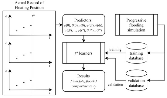
Figure 1.
Flowchart of the classification process.
- the final fate of the progressive flooding scenario: this is the most important information required by the master during a flooding emergency, thus shall be included in each onboard emergency DSS. The final fate is divided into the following classes: new equilibrium, sink, capsize, excessive heeling (final floating positions with large heel angles cannot be considered safe [17]);
- the flooded watertight compartments involved in the progressive flooding: the knowledge of the damaged main watertight compartments enable to immediately start the damage control procedures, helping to avoid uncontrolled floodwater spreading. The damage scenarios are mapped into a common response class if involve the same set of watertight compartments;
- the time-to-flood : this is the key information when the ship has to be abandoned. Hence, in nonsurvival scenarios, it shall be provided to the crew by an emergency DSS to enable proper planning of the ship evacuation.
The first two responses are classification problems that can be addressed by means of classification learners. On the contrary, being a numeral, regression learners can be employed to address the third problem.
Usually, as the damaged ship survives, the floating position reaches the new equilibrium with a decreasing pace that can be modelled, to a first approximation, a limited exponential trend [18]. Hence, in such cases, the accurate definition of is not an easy task. In some preliminary evaluations was observed that the large uncertainty connected to survival damage scenarios heavily affects the precision of the third problem. On the other hand, since all the other possible fates occur at a well defined time instant, the time-to-flood can be easily identified reducing the drawback on the regression accuracy. Hence, also considering that the time-to-flood is not essential in survival cases, only the lost-ship scenarios (sink, capsize, excessive heeling) have been here considered studying the third problem.
In all the cases, the predictors are the values of heel angle, trim angle and sinkage, recorded at constant time intervals . Hence, at each time , multiple of , three specific learners can be employed to forecast the damage scenario responses based on the past information (values of heel angle, trim angle and sinkage recorded up to ). During a real flooding scenario, the predictions are still valid during the next period. Then, another new floating position point is recorder adding the related three predictors that are employed by the next step learners to update the consequences predictions.
All the learners defined at each time instant are trained by means of a single database of progressive flooding simulations. The damage cases included in the database can be defined according to different methodologies, such as Monte Carlo (MC) sampling or a parametric definition. The main goal is anyhow to maximise the classification accuracy, which can be tested through a second validation database, generated independently from the training one.
2.2. Accuracy Evaluation
Considering a properly sized validation database, the accuracy of trained classifiers can be estimated. The accuracy rate of a classification algorithm is usually defined as the capability to assign a specific scenario from the validation database to the correct response class. Namely, considering a specific time instant , the accuracy of the related classifiers can be defined as:
where is the number of the correctly classified damage scenarios and N the total number of the scenarios induced in the validation database.
Due to the particular nature of the problem, which aims to predict the outcomes of the damage scenario, a so-called “ongoing accuracy” can be also defined excluding all the damage scenarios that have already reached the final stage ():
where is the number of the correctly classified ongoing damage scenarios and the total number of the ongoing scenarios induced in the validation database. In addition to the previously defined accuracy measures, also the confusion matrices have been here employed to deepen the analysis of the results.
Regarding the regression problems, the accuracy can be checked by means of several statistical indicators. Here, among the others the coefficient of determination has been employed:
where are the known responses, their mean values and the responses predicted by the model. Once again, an ongoing coefficient of determination has been also defined based only on the ongoing damage scenarios. Besides, the predicted-observed plot can be also evaluated at each time instant for better study the regression results.
2.3. Tested Machine Learning Algorithms
In this work, a quite large set of classification/regression algorithms have been tested to select the most effective one for the three studied problems. The tested methods can be divided into three families: decision trees, k-nearest neighbour and support vector machine. Hereinafter, they are briefly introduced.
2.3.1. Decision Trees
Decision Trees are well-known nonparametric supervised algorithms based on binary decisions. Decision trees can be used to perform both classification and regression (providing a piecewise approximation of the response function). The decision process is shaped like a tree, starting from a root and then moving node by node according to predictors values up to the leaves, i.e., the predicted response. The typical structure of a decision tree is reported in Figure 2. Starting from the route, the decisions are made among two possible directions according to the value of a single predictor . A similar process is carried out in each passed node along with the tree structure, until, decision by decision, a leaf is reached, corresponding to the response class.
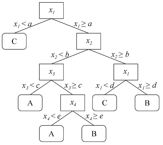
Figure 2.
Sketch of a simple decision tree.
Decision trees are trained with a dataset providing the relation between predictors and response, modelling the link between them. Here the following methods have been tested for the proposed studied classification problems:
- Decision Trees (DT): classification is performed by a single decision tree, applying Gini’s diversity index as impurity measure in the splitting criterion and testing all the predictors at each node to select the one that maximises the split-criterion gain [19];
- Least Square Boosted Decision Trees (DTLSB): the method is applied for regression problems employing a Least Squares (LS) boosting algorithm [20]. Here, 30 weak learners have been utilised, fitting at each step a new learner to the difference between the observed response and prediction coming from the already trained learners;
- Random Undersampling Boosted Decision Trees (DTRUSB): the method is applied only on classification problems and utilises a hybrid sampling/boosting algorithm to better deal with skewed training-data while assuring a limited computational effort [21]. Considering the studied problems, the final fate can easily result in a large majority of survival scenarios, leading to imbalanced training data. This is why, among the boosting algorithms present in literature, the Random Undersampling one has been here tested;
- Bagged Decision Trees (DTB): in this method, the problem is decomposed in a set of tree predictors, i.e., the random forest, where each tree depends on the values of a random and independently sampled vector with the same distribution for all trees in the forest. The preferred response is then selected according to the vote given by each tree in the forest. The method showed very good accuracy and robustness with respect to noise [22]. Hence, due to the uncertainties affecting the progressive flooding simulations [23,24], this method has been here considered.
2.3.2. K-Nearest Neighbour
K-nearest neighbour is a nonparametric family of learning algorithms where the response is assigned according to votes given by its neighbours or the mean value of their response for classification and regression problems respectively. The k parameter represents the number of the nearest neighbours involved in the evaluation of class membership or numerical response. This means that, if , the response related to a given set of predictors is equal to the one of its nearest neighbour, i.e., the training data point having the lower distance in the predictors’ space. The process is sketched in Figure 3 for a simple two-dimensional predictors’ space. For such a family of algorithms, the training phase is limited to storing and possibly standardise the training data, whereas the core of the algorithm is how the distance among single data points defined by predictors’ values is evaluated. Given two data points identified by predictors vectors and respectively, the following different algorithms employing different metrics have been here tested:
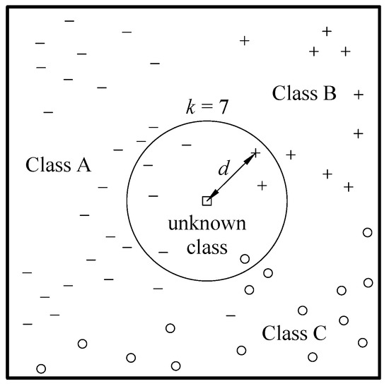
Figure 3.
Sketch of the behaviour of a K-Nearest Neighbour algorithm.
- K-Nearest Neighbour (KNN2): employing the Euclidean distance defined as:
- Cubic K-Nearest Neighbour (KNN3): employing the third-degree Minkoswki distance defined as:
- Cosine K-Nearest Neighbour (KNNC): employing the cosine distance defined as:
- Weighted K-Nearest Neighbour (KNNW): in this method, the Euclidean distance is still employed but a different weight is applied to each neighbour response. The closer is the neighbour the higher its response weight will be. Here, the applied weight is the squared inverse of the Euclidean distance.
In all the tested methods, the k parameter is assumed to equal 10 and the training data are standardised: for each predictor, the mean value and standard deviation are computed for centring and scaling the training data respectively.
2.3.3. Support Vector Machine
Support Vector Machines (SVM) are supervised learners algorithms based on statistical learning frameworks. The SVMs can be employed in both classification and regression problems.
Standard SVM classifiers are binary algorithms allowing to identifying the best hyperplane separating the elements belonging to two different classes. Considering a training dataset, the closest data points to the hyperplane are called support vector and the hyperplane is selected in order to maximise the margin between the two classes (Figure 4a), i.e., the distance between two parallel hyperplanes defining a region not containing any data point [25].
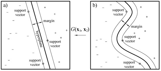
Figure 4.
Sketch of a binary Support Vector Machine (SVM) highlighting the behaviour of the kernel function mapping the space (b) to the (a) one.
Since SVMs classifiers are binary, a direct application to the studied classification problems is not possible as they involve three or more classes. A viable solution to employ binary classifiers in multiclass learning is the application of Error-Correcting Outputs Codes (ECOC). An ECOC model reduces a multiclass problem to a set of binary classification problems and it is based on a coding design and a decoding scheme. The coding design is a matrix defining which classes are trained by a specific binary learner. On the other hand, the decoding scheme aggregates the results of the single binary classifiers determining the prediction of the multiclass problem. Here, a one-versus-one coding design has been employed [26].
As mentioned, SVM can be employed also in regression problems [27]. In such a case the hyperplane is defined as the one that best fits the training data. Its equation is obtained minimising the norm value provided that fore each data point, all the prediction errors are inside an accepted error (feasible problem). Otherwise, for infeasible problems, slack variables are added to deal with data points having error greater than .
In certain problems, the separation among classes or the regression function cannot be defined by a simple hyperplane. For instance, Figure 4b qualitatively shows this problem for a binary classification problem. In such cases, the separating criterion can be reconducted to a hyperplane by applying a proper kernel function , mapping the original space into a higher-dimensional space [28]. Here, in order to find which kernel function best suits the studied classification problems, the following SVM algorithms have been tested:
- Linear Support Vector Machine (SVM1): employing a linear kernel function defined as:
- Quadratic Support Vector Machine (SVM2) employing a second order polynomial kernel function defined as:
- Cubic Support Vector Machine (SVM3): employing a second order polynomial kernel function defined as:
- Gaussian Support Vector Machine (SVMG): employing a radial basis function kernel defined as:
As done for the K-nearest neighbour algorithms, the training data are here again standardised.
3. Test Case
The proposed technique has been applied to a box-shaped barge in order to assess its feasibility. In the present section, the test geometry is introduced. Besides, training and validation databases of time-domain simulations of progressive flooding are also required. Hence, besides the adopted progressive flooding simulation technique, the generation of damage cases for the test geometry is presented to study the consequences of a ship-to-ship collision.
3.1. Test Geometry
The test arrangement is a box-shaped barge having five watertight compartments and three main decks. Table 1 provides the main particulars of the barge geometry and the intact condition. Figure 5 shows the general arrangement of the test geometry. The internal openings’ dimensions and location are provided in Table 2.

Table 1.
Main particulars of test case arrangement.
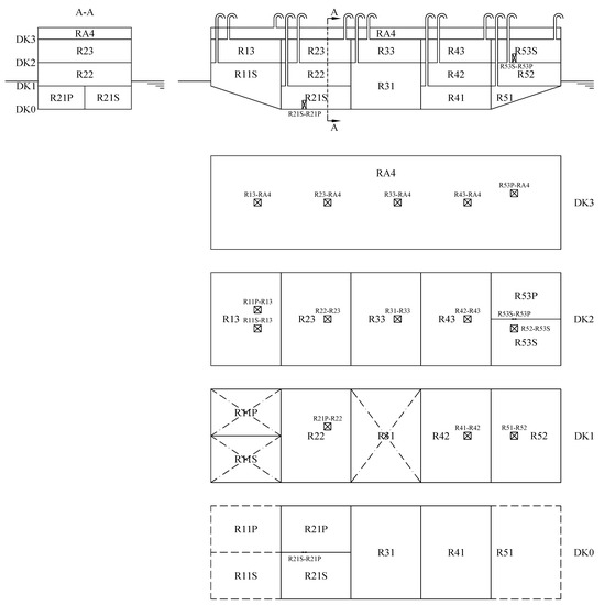
Figure 5.
General arrangement of the test geometry.
Table 2.
Main characteristics of the test case openings. is the centre of the opening in ship-fixed reference system.
The barge has a quite complex internal subdivision: lower rooms in first and third compartments extend across the lower deck and a partial longitudinal bulkhead is fitted within the first, second and fifth compartments. The main compartments are considered watertight up to the third deck fitted with a single room along the whole barge length. All the rooms are considered fully vented and are modelled with nonstructured triangular meshes to apply an in-house-build hydrostatic code based on pressure integration technique [29]. The internal openings as well as the breaches are also modelled with mashes and have a constant discharge coefficient .
3.2. Progressive Flooding Simulation
In order to generate the training and validation databases a flooding simulation technique is needed. Since this work aims at the prediction of damage consequences to provide decision support, there is no interest in a detailed simulation of the damage scenarios involving driving to a very fast capsize during the dynamic transient. In fact, in such a case, the time will be insufficient to apply any countermeasure to mitigate/avoid the consequences of the damage scenario. Hence, in this study, focus shall be made on the progressive flooding of the ship, where the process can be considered quasistatic [30].
In this work, a quasistatic simulation method has been then applied to generate the database, having also the advantage of a low computational load that enables a quite fast generation of large databases. The adopted progressive flooding method consists of a main simulation loop where the ship floating position is fixed over a variable integration time step . Hence, considering an earth fixed reference system having origin on the sea free surface, the floodwater levels and the waterheads can be defined as shown in Figure 6. The process is governed by the conservation of mass and the steady Bernoulli equation which can be written as:
where is the floodwater level in i-th room, and its permeability and free surface area respectively, while is the volume flowrate through the opening connecting the i-th and j-th rooms having area , discharge coefficient and distance of the lowest tip from sea free surface . Combining the Equations (11a) and (11b) a differential algebraic equation system can be obtained in the form:
where the differential part refers to the partially filled rooms and the algebraic one to the completely filled rooms having a waterhead . The algebraic part can be linearised in order to obtain an algebraic solution used to estimate the levels at the subsequent integration time step [18]. The solution reads:
where are the levels at the initial time instant and is the Jacobian matrix of the differential part of the System 12. Once the is defined according to an adaptive procedure based on floodwater level derivatives [16], the algebraic part can be solved as nonlinear equation system. Here, the Levenberg–Marquardt algorithm has been used [31].
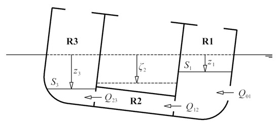
Figure 6.
Definition of the water levels z and waterheads for partially and completely filled rooms respectively [16].
3.3. Database Generation
Here, both the training and validation databases have been generated applying MC sampling in compliance with SOLAS, to study collision damage scenarios. According to SOLAS Ch.II, the damage is single, is assumed box-shaped and always crosses the waterline. The box can be defined with five parameters:
- damage length ;
- the longitudinal position of the damage centre ;
- damage penetration measured from shell side ();
- height of the higher tip of the damage above Base Line (BL);
- height of the lower tip of the damage above BL;
Using the MC method, once a probability distribution is defined for these parameters, it is possible to generate random damage scenarios accordingly [32]. SOLAS Ch.II provides the probability distributions for the first four parameters: , , b and . SOLAS does not define the probability distribution of , since the current probabilistic damage stability requirements use a worst-case-approach to deal with this parameter. However, to apply MC generation, the probability distribution necessary to define the lower limit of the damage box. Here, the formulation proposed in [33] is assumed, being complementary to the ones adopted by SOLAS. In fact, all the employed distributions have been obtained from statistical analysis on a database of real collision accidents collected by IMO. Hence, applying these probability distributions a SOLAS compliant database can be generated. In this preliminary study, the damage penetration has not been considered. Actually, only shell damages have been modelled assuming all internal structures as intact.
According to the presented assumptions, the following independently-generated databases have been generated for the test geometry:
- MC01: including 1000 damage cases (173 nonsurvival cases);
- MC02: including 2500 damage cases (398 nonsurvival cases);
- MC05: including 5000 damage cases (768 nonsurvival cases);
- MC10: including 10,000 damage cases (1544 nonsurvival cases);
- MC15: including 15,000 damage cases (2286 nonsurvival cases);
- MC20: including 20,000 damage cases (173 nonsurvival cases);
- MC30: including 30,000 damage cases (4686 nonsurvival cases);
- MC40: including 40,000 damage cases (6263 nonsurvival cases);
- MC50a: including 50,000 damage cases (7886 nonsurvival cases);
- MC50b: including 50,000 damage cases (8059 nonsurvival cases);
All the damage cases leading to ship capsize or to overtake the safe heel angle threshold are accounted beneath the nonsurvival ones. In all the databases, the simulations have been carried out up to 2250 s, since it is sufficient to include the time-to-flood of the large majority of the damage scenarios, as shown in Figure 7. In fact, for the test geometry, about 0.6% of damages has a time-to-flood exceeding the assumed maximum simulation time. Since, their final fate is unknown, these damage scenarios have been classified as “time exceeded”. The maximum simulation time is quite limited due to the test geometry, characterised by large volume rooms and wide free internal openings. Besides, applying SOLAS, the probability to obtain considerably large damages is quite high, as shown in Figure 8. Nevertheless, the maximum simulation time has been deemed sufficient to suit the purpose of the present study.
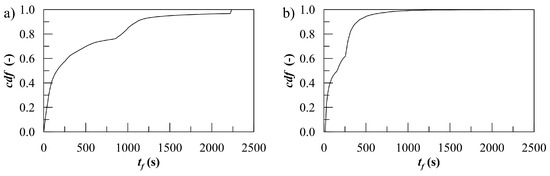
Figure 7.
Comulative density function of the time-to-flood in the MC50b database for all damage cases (a) and for nonsurvival ones (b).
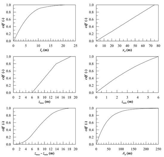
Figure 8.
Cumulative density functions of main damage characteristics in the MC50b database.
As mentioned, the adopted progressive flooding simulations method employs an adaptive time step [16]. Thus, the simulation results have been postprocessed to assess the predictors for learners: the heel angle trim angle and sinkage have been evaluated by interpolation assuming a constant time interval s.
4. Results and Discussion
Before testing the different learning methods, the effect of the database dimension on the accuracy of the classification/regression problems has been studied to select the proper number of damage cases to be included in the training database. To this end, all the generated databases (except for the MC50b) have been used as the training database, while the database MC50b as been always employed for validation. As an example, Figure 9 provides the results of such an analysis related to DTB method. Curves refer to different time instants within the maximum simulation time. It can be noted that almost all the curves converge to a maximum value of accuracy as the number of training damage cases increases. According to the results, the database MC20 has been chosen as the best training database, since only marginal gains on the ongoing accuracy of classification and regression results from higher N. Moreover, such gains can be obtained only at a high computational cost: databases have been generated with an Intel® Xeon® CPU E5-2630 v4 (2.20 GHz) workstation requiring about 1 h to simulate 1000 damage cases (18 threads running in parallel).
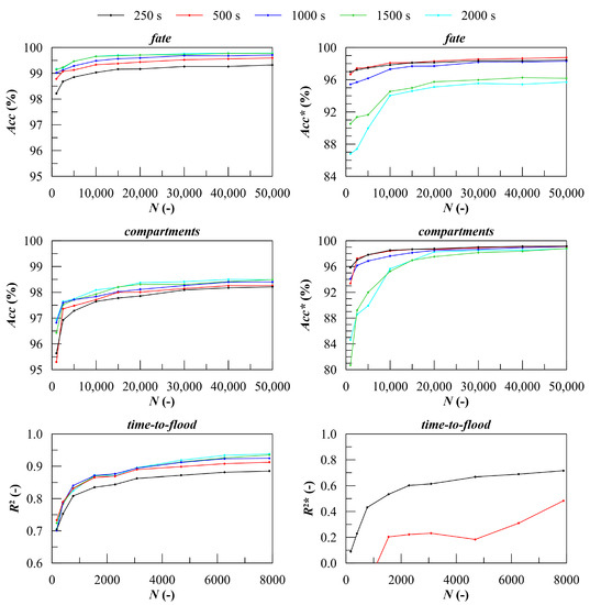
Figure 9.
Accuracy evaluated at different time instant as function of number of damage cases in the training database employing Bagged Decision Trees (DTB) classification technique. Validation: MC50b.
Figure 10 shows the results obtained by applying the studied learners trained with the database MC20 and again validated with the largest database MC50b. Both total and ongoing accuracy have been computed for the prediction of final fate and damaged compartments, whereas the total and ongoing determination coefficient has been evaluated for the time-to-flood regression. In general, the total accuracy of all the three problems is very good: for values converge to a practically constant maximum. Considering only the results related to ongoing damage scenarios, the behaviour is slightly different: the and increases constantly reaching a local maximum in an area defined by the number of still ongoing damage scenarios included in the training database. It can be noted that such an area spans within . Then, as the number of ongoing damage scenarios becomes lower than 20%, the ongoing performances decay, slightly for the two classification problems, more heavily for the time-to-flood regression. The considerations above yields for all the applied techniques, which, nevertheless, show different accuracy on the studied problems. In the following, they are discussed in more detail.
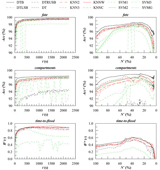
Figure 10.
Comparison of accuracy of different classification methods. Training: MC20; validation: MC50b.
Considering the first classification problem (ship final fate), the best performances have been obtained applying the DTB method that assures maximum accuracy of 99.8% and 98.6% for overall and ongoing, respectively, for the test geometry. Furthermore, the ongoing accuracy decay is quite limited since values are always above to 95.0%. The other classification algorithms show slightly lower performances and larger decay. The standard DT and the boosted DTRUSB provide almost the same results, being about 1% less accurate than the DTB. Regarding the K-nearest neighbours algorithms, all the tested metrics perform quite well. Better results can be obtained applying the weighted euclidean metric (KNNW), which has almost the same accuracy of the DT/DTRUSB techniques. About the support vector machines, the linear kernel (SVM1) is not capable to deal with the first classification problem. The best performances can be obtained with the quadratic (SVM2) and Gaussian (SVMG) kernel functions, which are anyhow slightly less accurate than the K-nearest neighbours algorithms. The SVM3 shows unstable behaviour for the studied problem. It is worth noticing that the SVM algorithms are not usually high-performance with a large predictor set. This problem has been so far observed here, compelling the reduction of predictors to obtain the results shown in Figure 10: for all SVM methods, the floating position has been recorded every 60 s instead of the 15 s time interval applied for all the other techniques. For the studied geometry, this value is a good compromise between the maximum value and the fast convergence of the accuracy to the constant maximum value.
Besides, some additional considerations can be drawn about misclassification. For the final fate problem, the most dangerous error (type I) is the selection of a survival scenario in case of ship capsize or excessive heeling. In fact, in such a case, a DSS based on machine learning might suggest the master not to evacuate the ship with imaginable consequences on people safety. Softer concerns are related to all other errors (type II) including also the misclassification of nonsurvival type. It has been observed that the type I error is a fraction of the type II ones for the tested geometry. For instance, Table 3 and Table 4 provide the confusion matrices evaluated at and , respectively.
Table 3.
Confusion matrix related to ship final fate evaluated at 250 s. Training: MC20; validation: MC50b.
Table 4.
Confusion matrix related to ship final fate evaluated at 500 s. Training: MC20; validation: MC50b.
Concerning the second classification problem (damaged watertight compartments), most of the considerations applying to the final fate still yield. The best performances are again obtained with DTB method, showing overall accuracy up to 98.4% and ongoing one up to 99.0%, which does not decline below 98%. A gap larger than 1% separates the accuracy of all the other techniques. With respect to the first problem, it shall be noticed that the boosted trees perform very poorly to identify the damaged compartments. On the contrary, the SVM2 method performs quite well, giving results comparable to the DT and KNNW ones. Moreover, the SVMG does not provide good results, especially at the very beginning of the flooding process. This suggests that the studied classification problem cannot be described well by a radial basis kernel as well as by a linear one. Eventually, higher instability has been found applying the cubic SVM3 method.
Regarding misclassification, the second problem has been proven to be somehow more resilient than the first one, although the accuracy seems lower at a first glimpse. In fact, as shown in Table 5 and Table 6, the classification errors are not usually related to completely wrong identification of the damaged compartments set but mostly to neglecting in an initial flooding phase one of the damaged compartments. This likely happened when the damage affecting one watertight compartment is considerably smaller than the one(s) affecting the other damaged compartment(s). However, this kind of error tends to vanish as a sufficiently large volume of floodwater is loaded, so as the effect of the initially neglected compartments become more relevant.
Table 5.
Confusion matrix related to damaged compartments evaluated at 250 s. Training: MC20; validation: MC50b.
Table 6.
Confusion matrix related to damaged compartments evaluated at 500 s. Training: MC20; validation: MC50b.
The results of regression on the time-to-flood for nonsurvival scenarios presents some relevant differences compared to the classification problems ones presented above. First, the decay of ongoing accuracy is more pronounced, leading to null values of when ongoing damages are less than 2% of the total damage cases in the training database. Moreover, due to the distribution of the time-to-flood in nonsurvival scenarios (Figure 7), such a condition occurs at about . Moreover, for the third problem, a clear preference for a method cannot be identified: both DTB and KNNW methods can be employed providing the best performances in the initial and final phase of progressive flooding, respectively. Both the methods reach a maximum value of the at about 250 s (corresponding to the 40% of ongoing damage cases in training database).
However, the ongoing value of determination coefficient is much reduced compared to the overall one: for DTB method the maximum values are and whereas the for KNNW and . The other methods perform more poorly. In particular, the SVM methods are very ineffective and only the Gaussian kernel shows a limited forecast capability, showing that data cannot be effectively separated with linear, quadratic or cubic kernel functions.
To better analyse the forecast capability of the two best algorithms the predicted-observed plots evaluated at and are provided in Figure 11 and Figure 12. The coloured part of the diagrams relates to forecasting () and it is divided into a red region and a green one. In the former, the time-to-flood is overestimated whereas in the latter is underestimated. Considering an onboard application for decision support purposes, the time-to-flood overestimation is very dangerous, since it could lead to slow down evacuation procedures. Hence, the latter could be not completed when the ship capsizes or reaches an unsafe condition. On the other hand, underestimation might rush the evacuation procedures, which can anyway imply a risk for passengers and crew but at lower levels. The plots show that applying both best methods, the predictions tend to group nearby the diagonal as the time proceeds, assuring increased reliability. However, due to the reduced number of damage cases having long duration included in the training database, all the employed methods show large errors for the largest time-to-floods, affecting the too. In particular, for the studied geometry, the DTB method, which provides a piecewise approximated regression, does not predict any value over 1104 s. The KNNW has no such a limitation. This is why it provides better results with less than 10% of ongoing damage cases in the training database. However, the low density of damage cases in this region cannot anyway assure high precision, leading to the decay, although somehow delayed. In conclusion, all the results obtained in this feasibility study pointed out that the distribution of the time-to-flood in the training database has a strong influence on the learners’ performances, in particular for the time-to-flood regression. To limit or avoid the ongoing accuracy decay, the SOLAS probability distributions are not appropriate for the studied geometry which shall be anyway used for validation purposes, being so far the most representative of realistic collision damages.
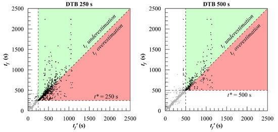
Figure 11.
Predicted over observed values of the time-to-flood computed at 250 s and 500 s from damage occurrence according DTB method. Training: MC20; validation: MC50b.
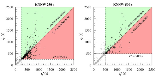
Figure 12.
Predicted over observed values of the time-to-flood computed at 250 s and 500 s from damage occurrence according to KNNW method. Training: MC20; validation: MC50b.
5. Conclusions
This work presented a novel approach to predict the flooding consequences by employing machine learning. The results show that it is possible to forecast the ship final fate, the damaged compartments set and roughly estimate the time to flood from the time evolution of the damaged ship floating position. Such a solution is thus applicable onboard for decision support purposes, without requiring the costly installation of a flooding detection system. Moreover, through the adoption of an independent validation database based on SOLAS probability distribution, it is also possible to measure and study the prediction accuracy that can be reported to the master.
The tested algorithms set does not pretend to thoroughly investigate all the classification algorithms available in the literature. Other techniques might be tested in future works trying to improve the present results. In particular, regarding time-to-flood, instead regression learners, neural networks could be tested. However, the set of tested methods is quite large and varied allowing to draw some preliminary conclusions about which are the most promising methods for the prediction of progressive flooding consequences.
For the tested geometry and applying SOLAS probability distributions for database generation, the best choice is represented by bagged decision trees, which shows very good accuracy for the classification of ship final fate and in identifying the damaged compartments. They can be employed also for time to flood regressions although the forecast is not very reliable for large time-to-floods. For the time being, weighted K-nearest neighbours should be preferred to address the latter problem, assuring a better accuracy on the prediction of longest damage scenarios.
Although the results obtained in this first work are promising, it shall be noticed that further study is still required on several aspects before onboard application. Namely, it is advisable to study the effect of the application of different probability distribution in the training database definition to prevent or reduce the decay of ongoing accuracy. For instance, different types of uniform distributions could be tested as well as the ones related to grounding damages, that are not currently considered within SOLAS. Furthermore, the method has been here tested on a barge geometry and should be tested on real passenger ship, which can be considerably more challenging. In fact, in a real environment, the flooding process can be affected by the uncertainty on several parameters, such as the discharge coefficients, the permeabilities and the loading condition. These issues have been not yet considered and should be addressed to increase the robustness of the proposed methodology.
Author Contributions
Conceptualisation, M.V., J.P.-O. and L.B.; methodology, L.B. and M.V.; software, L.B.; validation, L.B. and M.V.; formal analysis, L.B. and M.V.; investigation, L.B.; resources, L.B.; data curation, L.B.; writing—original draft preparation, L.B.; writing—review and editing, J.P.-O. and M.V.; visualisation, L.B., M.V. and J.P.-O.; supervision, J.P.-O. and M.V.; project administration, J.P.-O.; funding acquisition, J.P.-O. All authors have read and agreed to the published version of the manuscript.
Funding
This work has been fully supported by the Croatian Science Foundation under the project IP-2018-01-3739.
Institutional Review Board Statement
Not applicable.
Informed Consent Statement
Not applicable.
Data Availability Statement
Data is contained within the article.
Acknowledgments
This work was also supported by the University of Rijeka (project no. uniri-tehnic-18-18 1146 and uniri-tehnic-18-266 6469).
Conflicts of Interest
The authors declare no conflict of interest.
References
- Braidotti, L.; Degan, G.; Bertagna, S.; Bucci, V.; Marinò, A. A Comparison of Different Linearized Formulations for Progressive Flooding Simulations in Full-Scale. Procedia Comput. Sci. 2021, 180, 219–228. [Google Scholar] [CrossRef]
- Nasso, C.; Bertagna, S.; Mauro, F.; Marinò, A.; Bucci, V. Simplified and advanced approaches for evacuation analysis of passenger ships in the early stage of design. Brodogradnja 2019, 70, 43–59. [Google Scholar] [CrossRef]
- Ruponen, P.; Pennanen, P.; Manderbacka, T. On the alternative approaches to stability analysisin decision support for damaged passenger ships. WMU J. Marit. Aff. 2019, 18, 477–494. [Google Scholar] [CrossRef]
- Ölçer, A.; Majumder, J. A Case-based Decision Support System for Flooding Crises Onboard Ships. Qual. Reliab. Eng. Int. 2006, 22, 59–78. [Google Scholar] [CrossRef]
- Kang, H.; Choi, J.; Yim, G.; Ahn, H. Time Domain Decision-Making Support Based on Ship Behavior Monitoring and Flooding Simulation Database for On-Board Damage Control. In Proceedings of the 27th International Ocean and Polar Engineering Conference, San Francisco, CA, USA, 25–30 June 2017. [Google Scholar]
- Hu, L.; Ma, K. Genetic algorithm-based counter-flooding decision support system for damaged surface warship. Int. Shipbuild. Prog. 2008, 55, 301–315. [Google Scholar]
- Varela, J.; Rodrigues, J.; Guedes Soares, C. On-board Decision Support System for Ship Flooding Emergency Response. Procedia Comput. Sci. 2014, 29, 1688–1700. [Google Scholar] [CrossRef]
- Ruponen, P.; Pulkkinen, A.; Laaksonen, J. A method for breach assessment onboard a damaged passenger ship. Appl. Ocean Res. 2017, 64, 236–248. [Google Scholar] [CrossRef]
- Dankowski, H.; Krüger, S. A Fast, Direct Approach for the Simulation of Damage Scenarios in the Time Domain. In Proceedings of the 11th International Marine Design Conference—IMDC 2012, Glasgow, Scotland, 11–14 June 2012. [Google Scholar]
- Ruponen, P.; Larmela, M.; Pennanen, P. Flooding Prediction Onboard a Damage Ship. In Proceedings of the 11th International Conference on the Stability of Ships and Ocean Vehicles, Athens, Greece, 23–28 September 2012; pp. 391–400. [Google Scholar]
- Rodrigues, J.; Guedes Soares, C. A generalized adaptive mesh pressure integration technique applied to progressive flooding of floating bodies in still water. Ocean Eng. 2015, 110, 140–151. [Google Scholar] [CrossRef]
- Ruponen, R.; Lindroth, D.; Routi, A.; Aartovaara, M. Simulation-based analysis method for damage survivability of passenger ships. Ship Technol. Res. 2019, 66, 180–192. [Google Scholar] [CrossRef]
- Karolius, K.; Cichowicz, J.; Vassalos, D. Risk-based positioning of Flooding Sensors to reduce prediction uncertanty of damage survivability. In Proceedings of the 13th International Conference on the Stability of Ships and Ocean Vehicles-STAB 2018, Kobe, Japan, 16–21 September 2018; pp. 627–637. [Google Scholar]
- IMO. MSC.1/Circ.1291 Guidelines for Flooding Detection Systems on Passenger Ships; International Maritime Organisation: London, UK, 2008. [Google Scholar]
- Trincas, G.; Braidotti, L.; De Francesco, L. Risk-Based System to Control Safety Level of Flooded Passenger Ship. Brodogradnja 2017, 68, 31–60. [Google Scholar] [CrossRef]
- Braidotti, L.; Mauro, F. A Fast Algorithm for Onboard Progressive Flooding Simulation. J. Marit. Sci. Eng. 2020, 8, 369. [Google Scholar] [CrossRef]
- IMO. SOLAS 2018 Consolidated Edition; Chapter Ch.II-1 Part B Subdivision and Stability; International Maritime Organisation: London, UK, 2018. [Google Scholar]
- Braidotti, L.; Mauro, F. A New Calculation Technique for Onboard Progressive Flooding Simulation. Ship Technol. Res. 2019, 66, 150–162. [Google Scholar] [CrossRef]
- Breiman, L.; Friedman, J.; Olshen, R.A.; Stone, C.J. Classification and Regression Trees; CRC Press: Boca Raton, FL, USA, 1984. [Google Scholar]
- Hastie, T.; Tibshirani, R.; Friedman, J. The Elements of Statistical Learning, 2nd ed.; Springer: New York, NY, USA, 2008. [Google Scholar]
- Seiffert, C.; Khoshgoftaar, T.M.; Hulse, J.; Napolitano, A. RUSBoost: Improving clasification performance when training data is skewed. In Proceedings of the 19th International Conference on Pattern Recognition, Tampa, FL, USA, 8–11 December 2008; pp. 1–4. [Google Scholar]
- Breiman, L. Random Forests. Mach. Learn. 2001, 45, 5–32. [Google Scholar] [CrossRef]
- Rodrigues, J.; Lavrov, A.; Hinostroza, M.; Guedes Soares, C. Experimental and numerical investigation of the partial flooding of a barge model. Ocean Eng. 2018, 169, 586–603. [Google Scholar] [CrossRef]
- Braidotti, L.; Marinò, A.; Bucci, V. On the Effect of Uncertainties on Onboard Progressive Flooding Simulation. In Proceedings of the 3rd International Conference on Nautical and Maritime Culture-CNM 2019, Naples, Italy, 14–15 November 2019; pp. 21–30. [Google Scholar] [CrossRef]
- Christianini, N.; Shawe-Taylor, J. An Introduction to Support Vector Machines and Other Kernel-Based Learning Methods; Cambridge University Press: Cambridge, UK, 2000. [Google Scholar]
- Escalera, S.; Pujol, O.; Radeva, P. Separability of ternary codes for sparse designs of error-correcting output codes. Pattern Recognit. Lett. 2009, 30, 285–297. [Google Scholar] [CrossRef]
- Vapnik, V. The Nature of Statistical Learning Theory; Springer: New York, NY, USA, 1995. [Google Scholar]
- Scholkopf, B.; Smola, A. Learning with Kernels: Support Vector Machines, Regularization, Optimization and Beyond, Adaptive Computation and Machine Learning; The MIT Press: Cambridge, MA, USA, 2002. [Google Scholar]
- Braidotti, L.; Trincas, G.; Bucci, V. Analysis of the Influence of Pressure Field on Accuracy for Onboard Stability Codes. In Proceedings of the 19th International Conference on Ships and Maritime Research-NAV 2018, Trieste, Italy, 20–22 June 2018; pp. 80–87. [Google Scholar] [CrossRef]
- Ruponen, P. Progressive Flooding of a Damaged Passenger Ship. Ph.D. Thesis, Helsinki University of Technology, Helsinki, Finland, 2007. [Google Scholar]
- Hansen, P.; Pereyra, V.; Scherer, G. Least Squares Data Fitting with Applications; Johns Hopkins University Press: Baltimore, MD, USA, 2013. [Google Scholar]
- Kruger, S.; Dankowsky, H. A Monte Carlo based simulation method for damage stability problems. In Proceedings of the 38th International Conference on Ocean, Offshore and Arctic Engineering-OMAE 2019, Glasgow, Scotland, UK, 9–14 June 2019. [Google Scholar]
- Bulian, G.; Cardinale, M.; Francescutto, A.; Zaraphonitis, G. Complementing SOLAS damage ship stability framework with a probabilistic description for the extent of collision damage below the waterline. Ocean Eng. 2019, 186, 106073. [Google Scholar] [CrossRef]


Publisher’s Note: MDPI stays neutral with regard to jurisdictional claims in published maps and institutional affiliations. |
© 2021 by the authors. Licensee MDPI, Basel, Switzerland. This article is an open access article distributed under the terms and conditions of the Creative Commons Attribution (CC BY) license (http://creativecommons.org/licenses/by/4.0/).