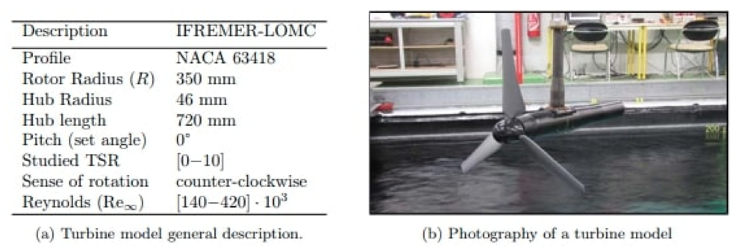
Figure 1.
General characteristics (
a) and design (
b) of the IFREMER-LOMC turbine [
21], University of Le Havre, 2013.
Figure 1.
General characteristics (
a) and design (
b) of the IFREMER-LOMC turbine [
21], University of Le Havre, 2013.
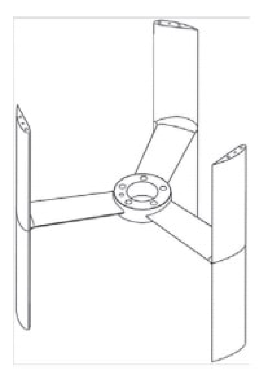
Figure 2.
Geometry of the Darrieus tidal turbine [
22], University of Grenoble, 2011.
Figure 2.
Geometry of the Darrieus tidal turbine [
22], University of Grenoble, 2011.
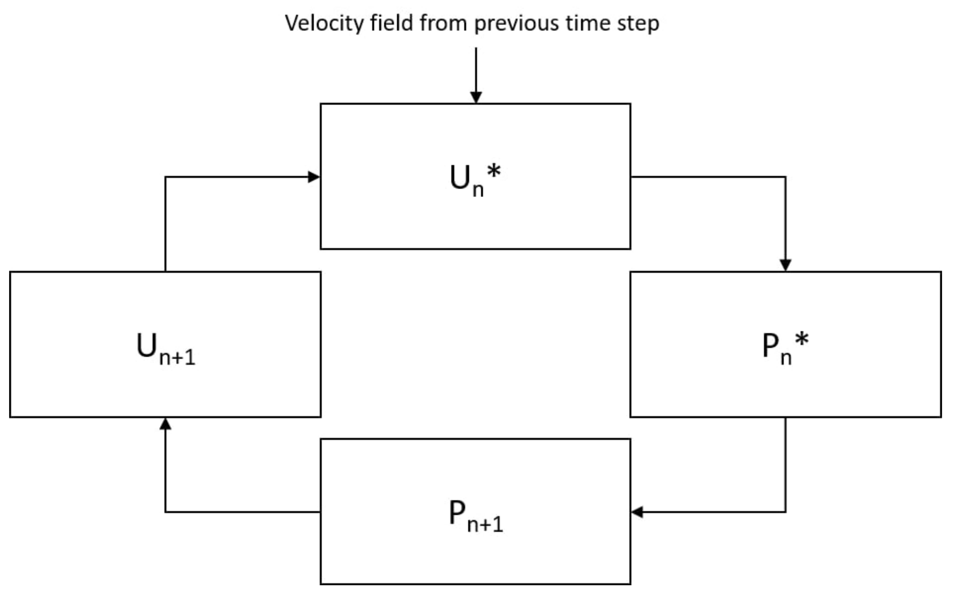
Figure 3.
Scheme of one iteration of PimpleFoam performed and repeated until the reaching of the convergence criteria. and are, respectively, the estimate of the velocity matrix and pressure matrix. and are the corrected pressure and velocity fields at iteration n.
Figure 3.
Scheme of one iteration of PimpleFoam performed and repeated until the reaching of the convergence criteria. and are, respectively, the estimate of the velocity matrix and pressure matrix. and are the corrected pressure and velocity fields at iteration n.
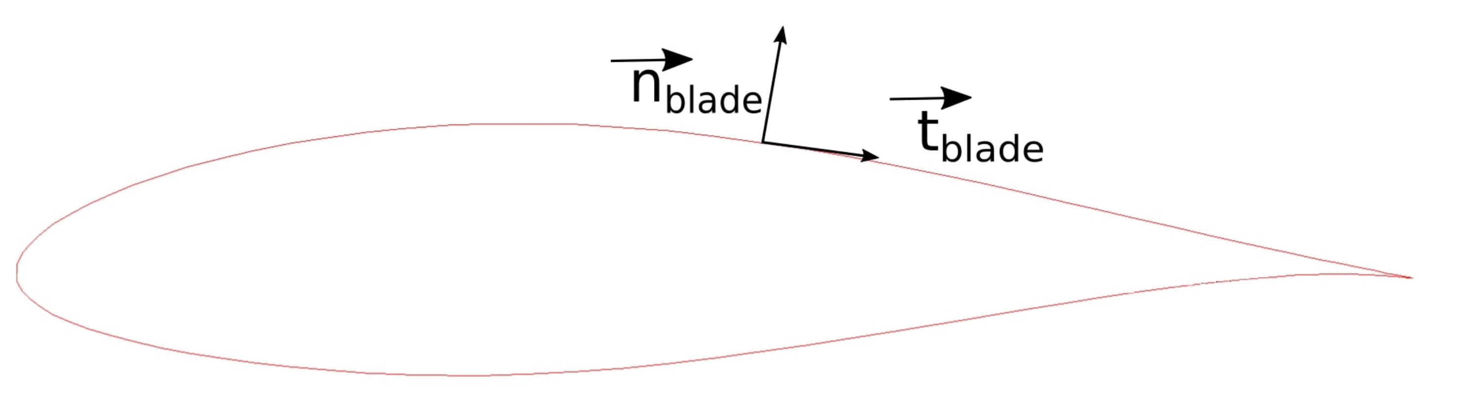
Figure 4.
and for a blade profile (red line).
Figure 4.
and for a blade profile (red line).
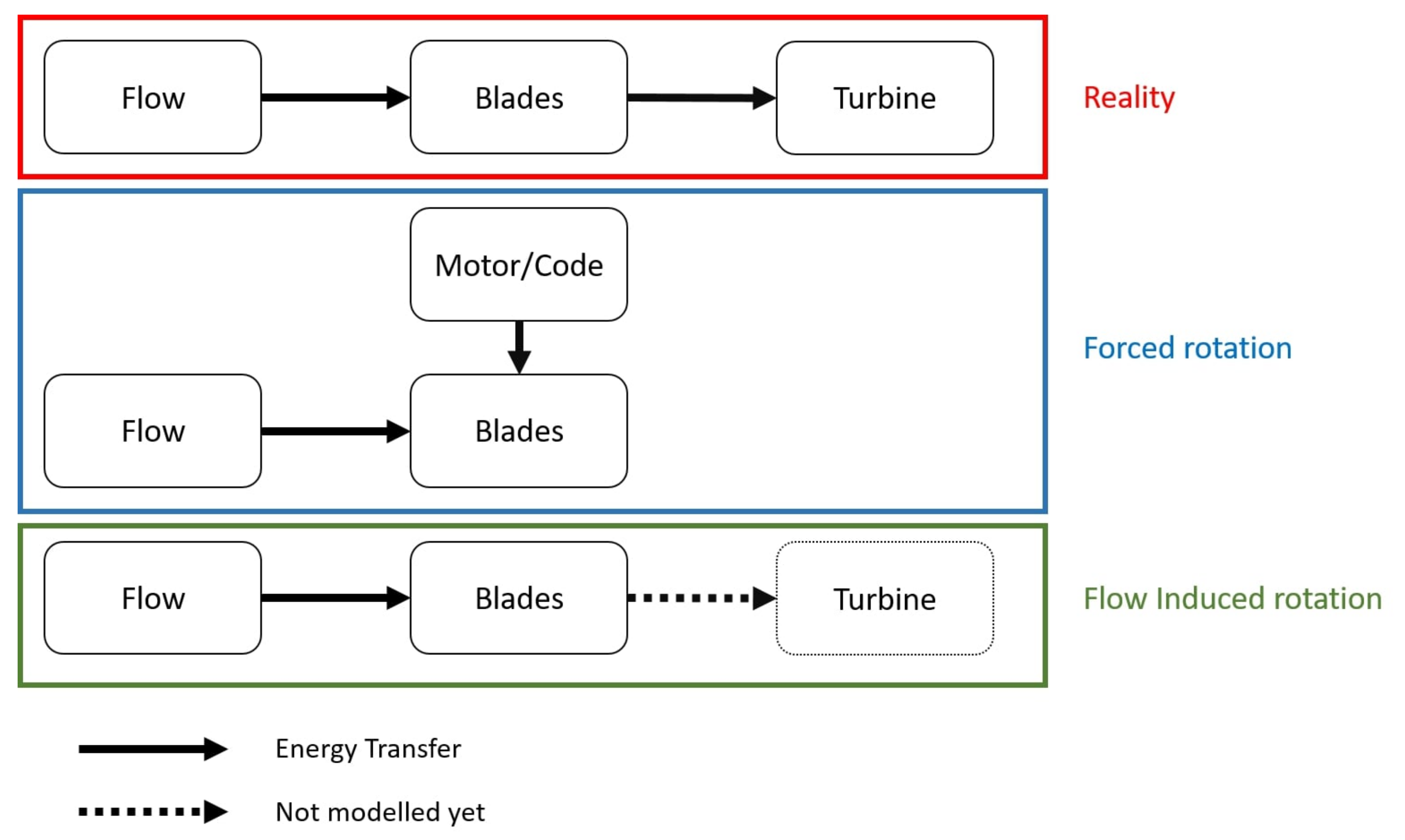
Figure 5.
Energy recovery chain for real life (red box), the forced rotation (blue box) and the flow induced rotation (green box). Black arrows represent the energy transfer.
Figure 5.
Energy recovery chain for real life (red box), the forced rotation (blue box) and the flow induced rotation (green box). Black arrows represent the energy transfer.
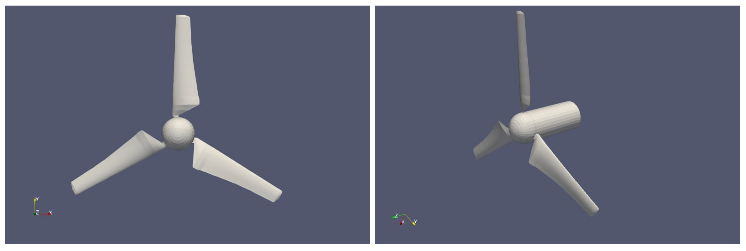
Figure 6.
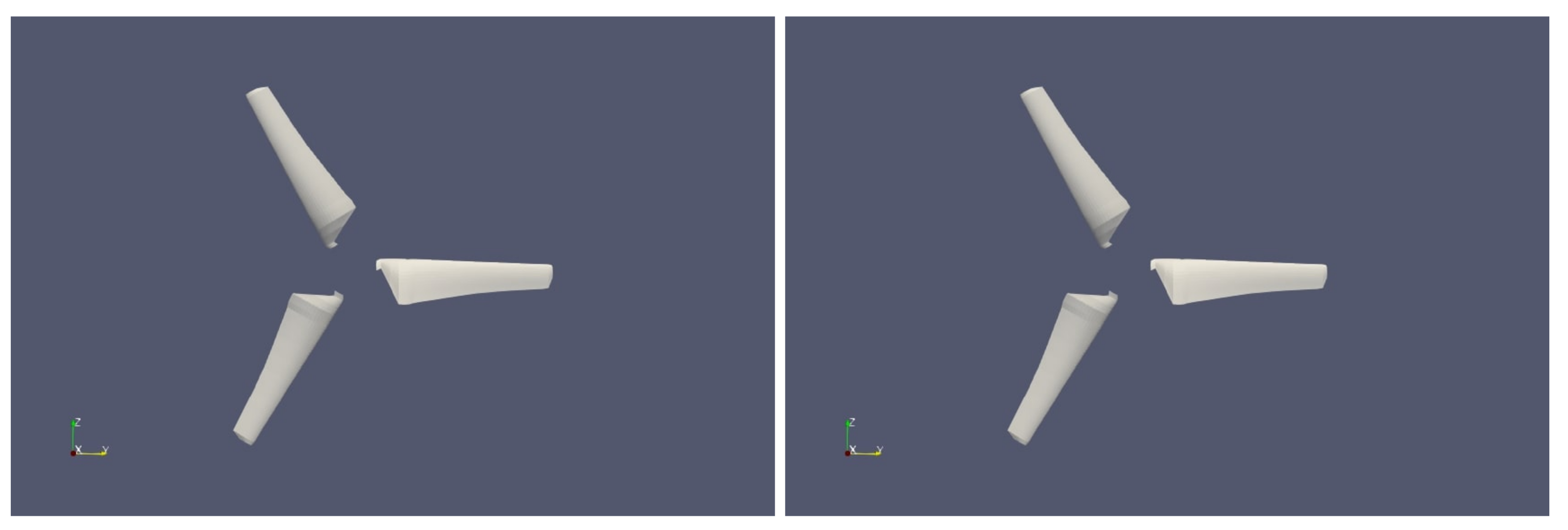
Three-dimensional views of the horizontal tidal turbine with a hub: front (left panel) and sideways (right panel) views.
Figure 6.
Three-dimensional views of the horizontal tidal turbine with a hub: front (left panel) and sideways (right panel) views.
Figure 7.
Same legend as for previous figure but without a hub.
Figure 7.
Same legend as for previous figure but without a hub.
Figure 8.
View of the X–Y plane of the computational domain with boundary conditions. D is the rotor diameter. U is the flow velocity in
, P is the pressure in
, and
is the pressure at the calculated point closest to the wall. The red square delimits the arbitary mesh interface (AMI) zone, and the blue circle shows the rotor position. The two black lines (1.2D and 2D) and the black cross are the extraction lines and the probe, respectively, used in the model validation in
Section 3.2.
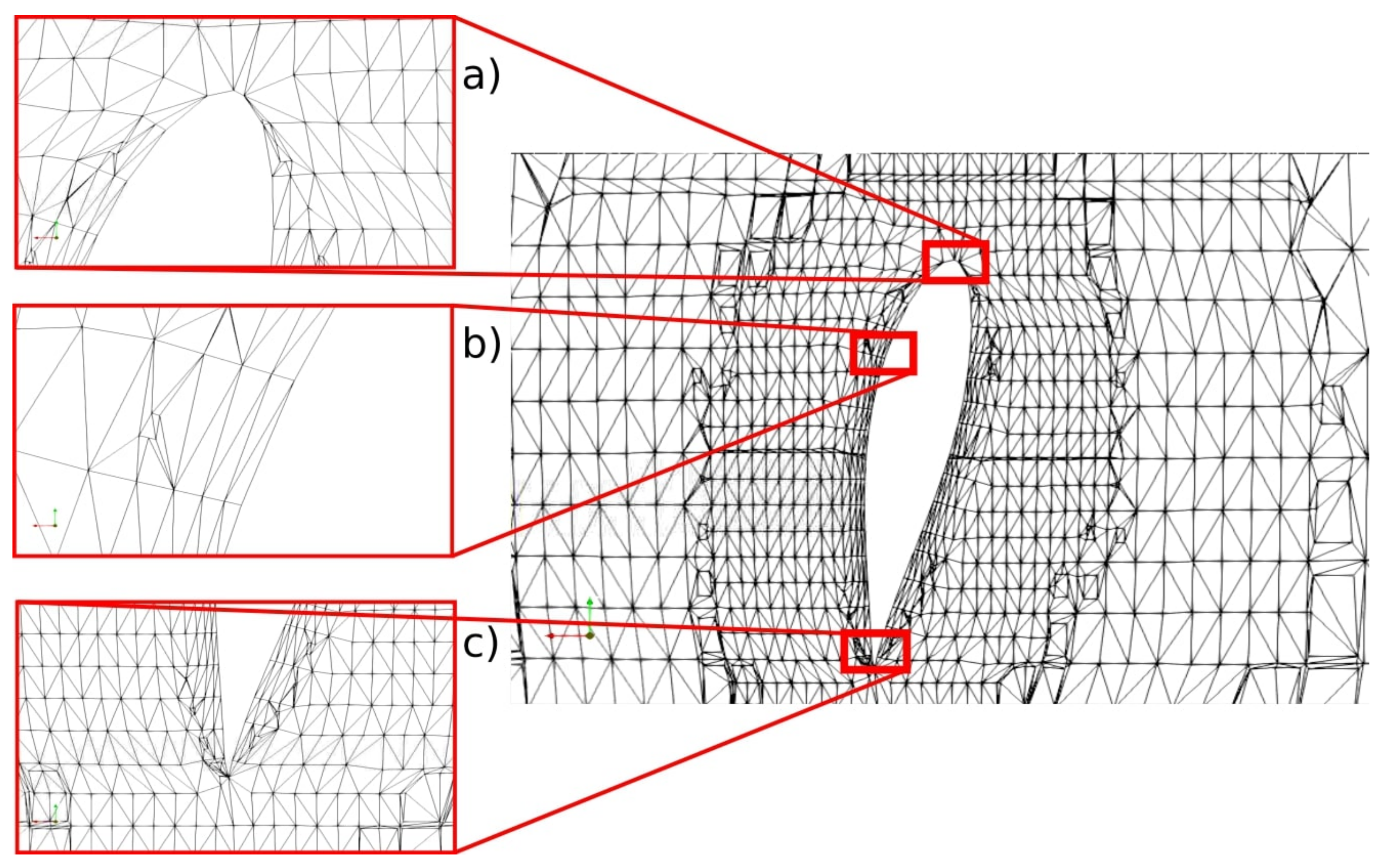
Figure 9.
Blade section for a level 5 refinement—the coarsest mesh (#2.1) with a close-up on leading edge (a), trailing edge (c) and upper surface (b). Distorted elements are due to the visualization section.
Figure 9.
Blade section for a level 5 refinement—the coarsest mesh (#2.1) with a close-up on leading edge (a), trailing edge (c) and upper surface (b). Distorted elements are due to the visualization section.
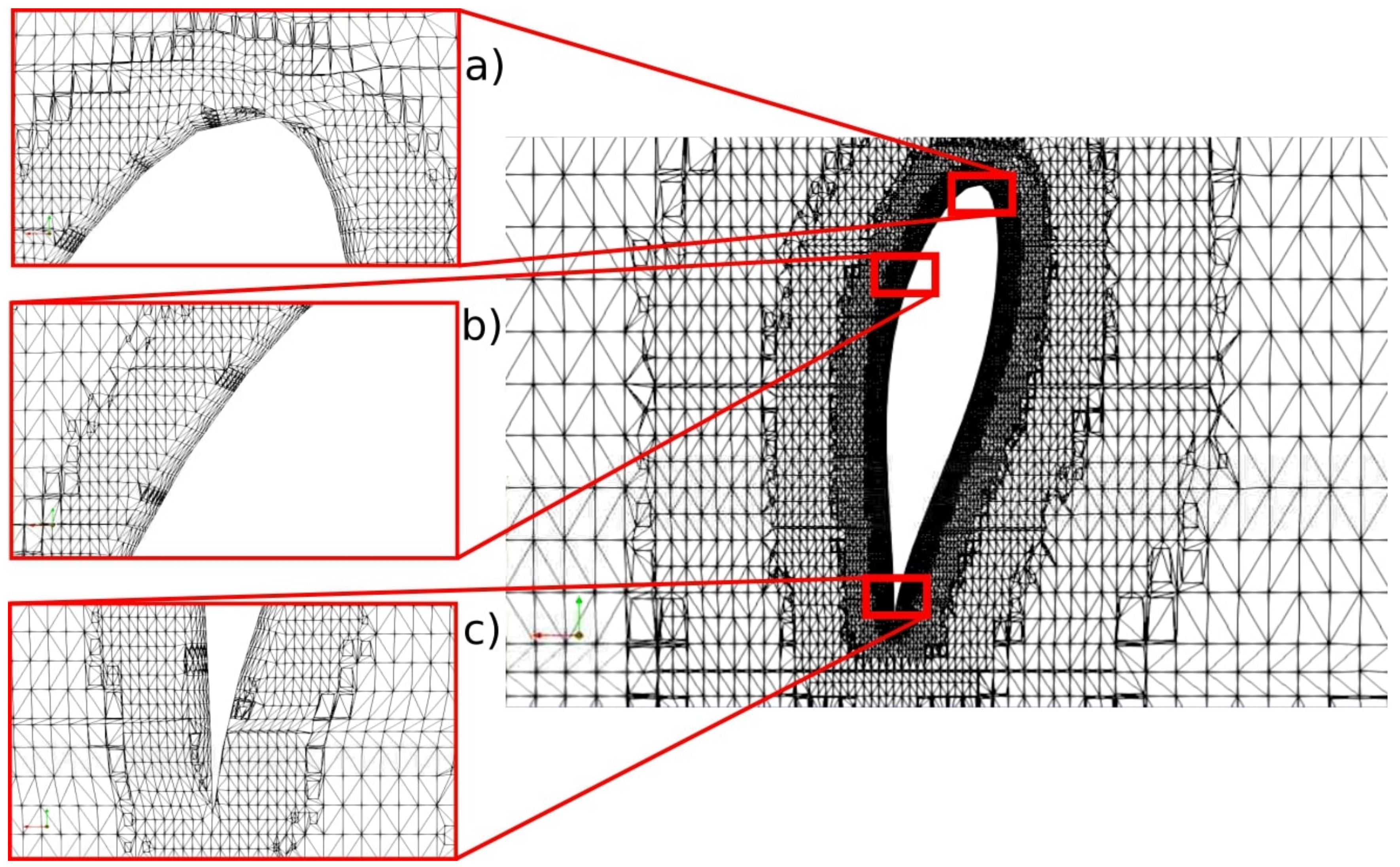
Figure 10.
Blade section for a level 9 refinement—the finest mesh (#2.4) with a close-up on leading edge (a), trailing edge (c) and upper surface (b). Distorted elements are due to the visualization section.
Figure 10.
Blade section for a level 9 refinement—the finest mesh (#2.4) with a close-up on leading edge (a), trailing edge (c) and upper surface (b). Distorted elements are due to the visualization section.
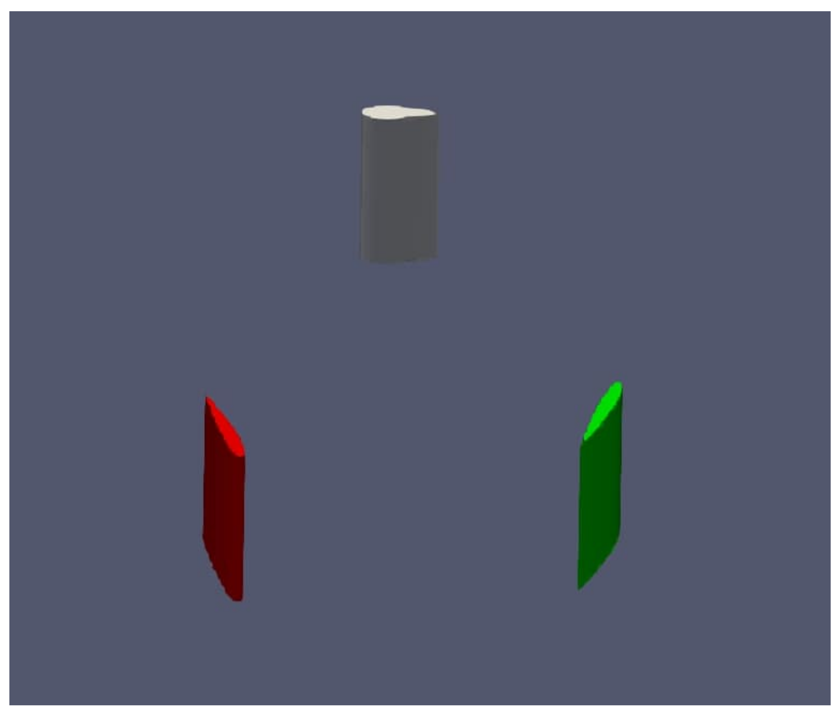
Figure 11.
Three-dimensional geometry of the blades of the vertical axis tidal turbine without hub for a sideways view.
Figure 11.
Three-dimensional geometry of the blades of the vertical axis tidal turbine without hub for a sideways view.
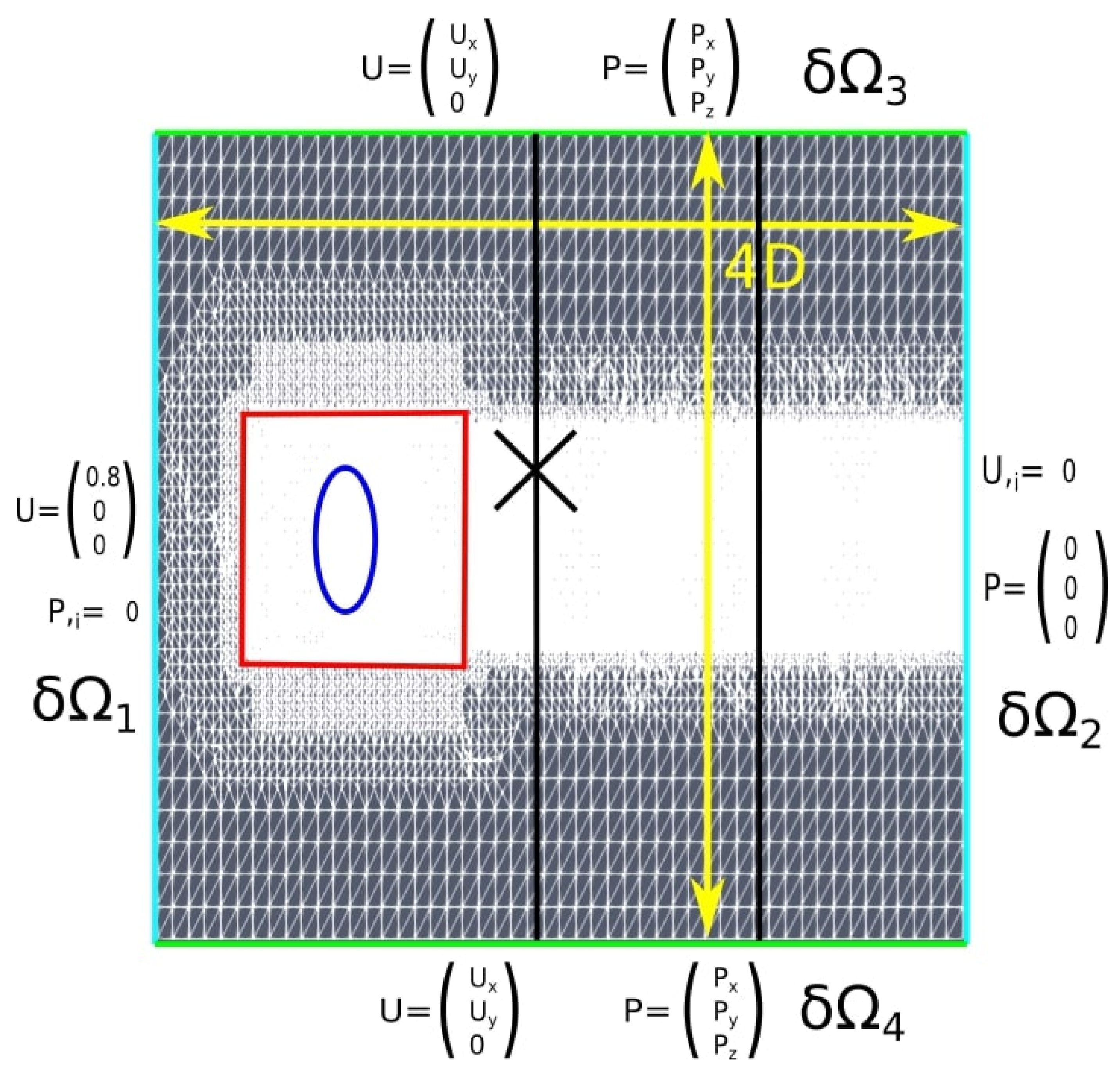
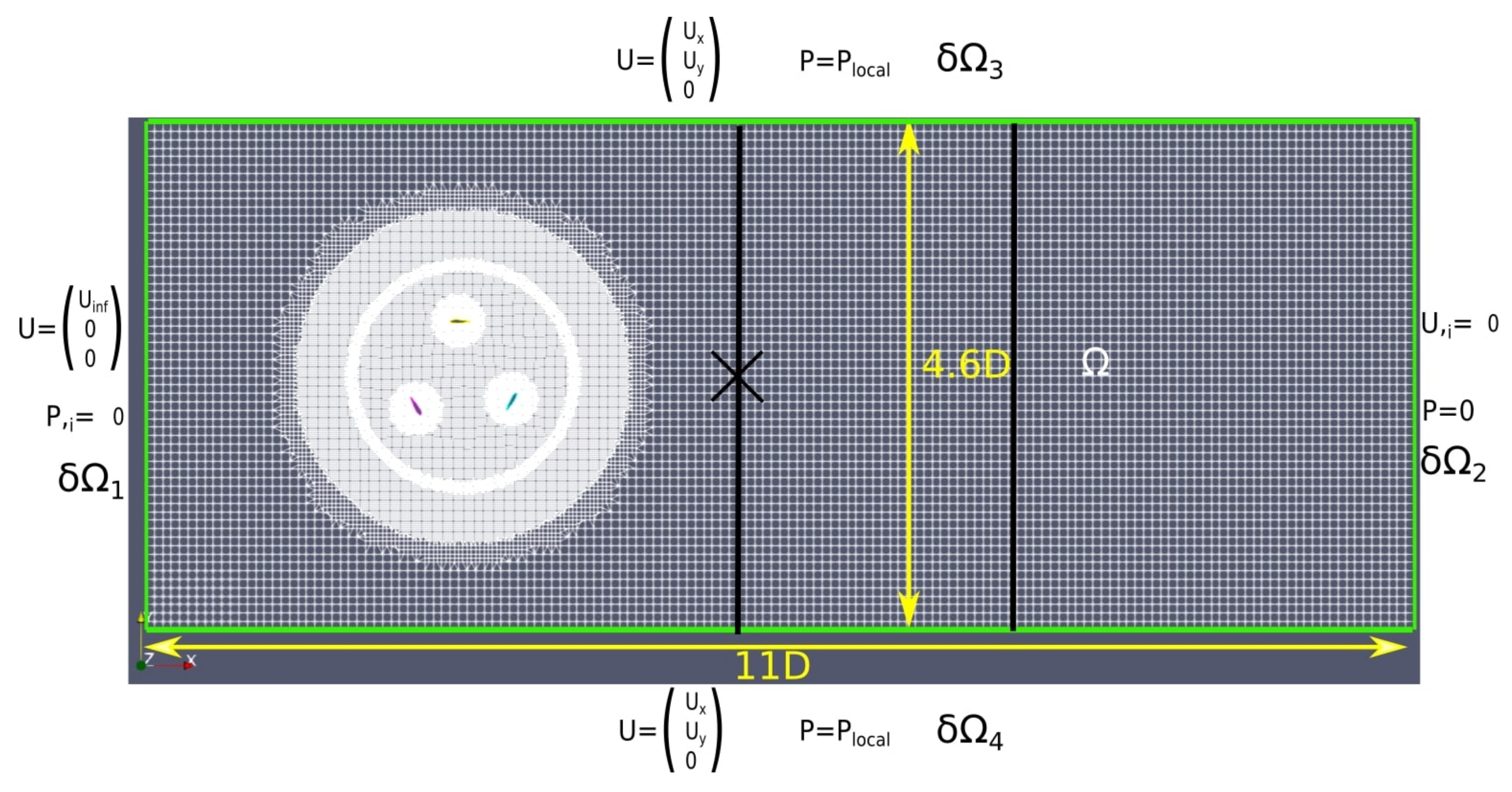
Figure 12.
View of X–Y plane for the computational domain with boundary conditions (in green). D is the rotor’s diameter in
. U is the flow velocity in
, and P is the pressure in
. The two black lines (2D and 4D) and the black cross are the extraction lines and the probe, respectively, used in the model validation in
Section 3.2.
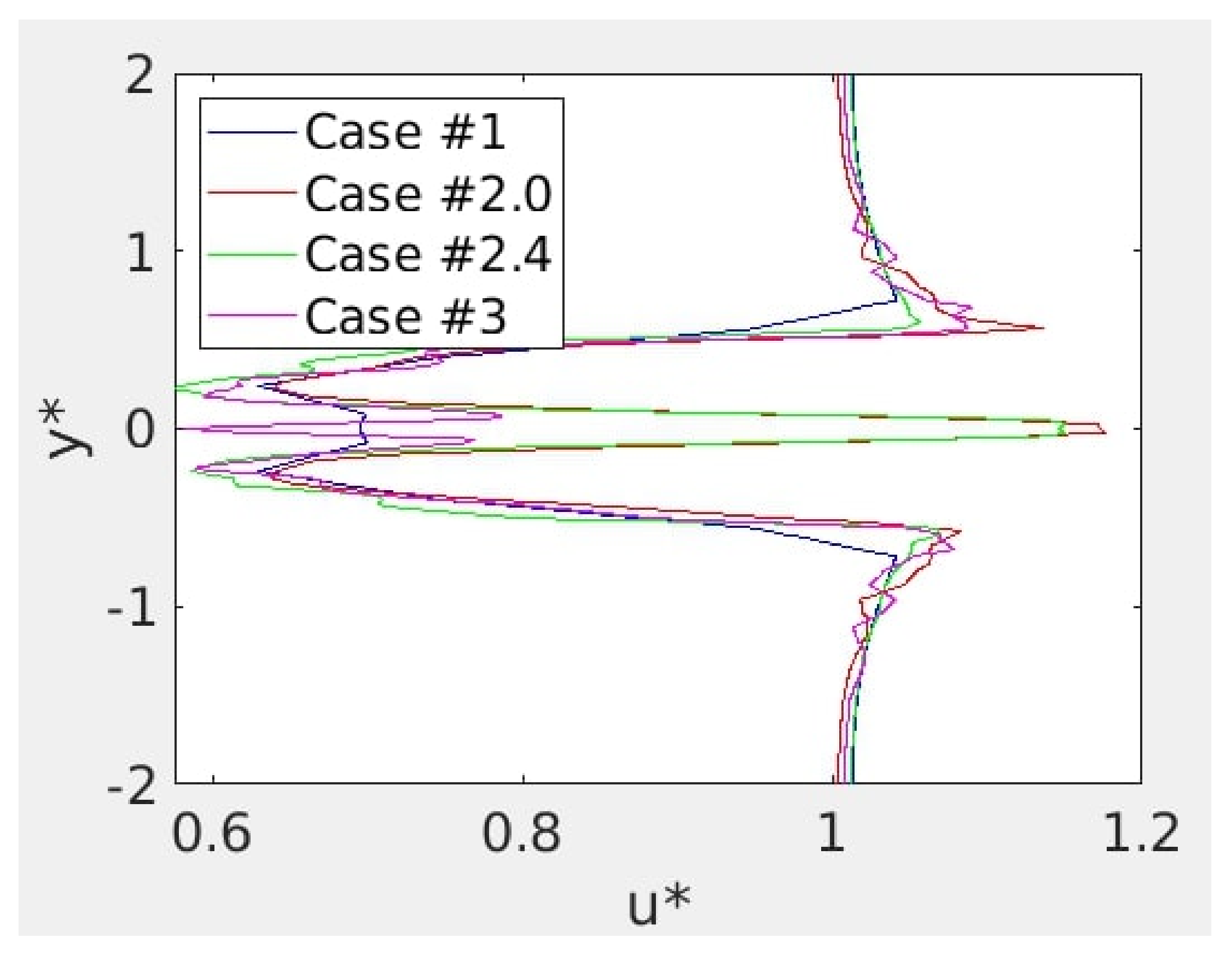
Figure 13.
magnitude along for #1, #2.0, #2.4 and #3 at = 1.2.
Figure 13.
magnitude along for #1, #2.0, #2.4 and #3 at = 1.2.
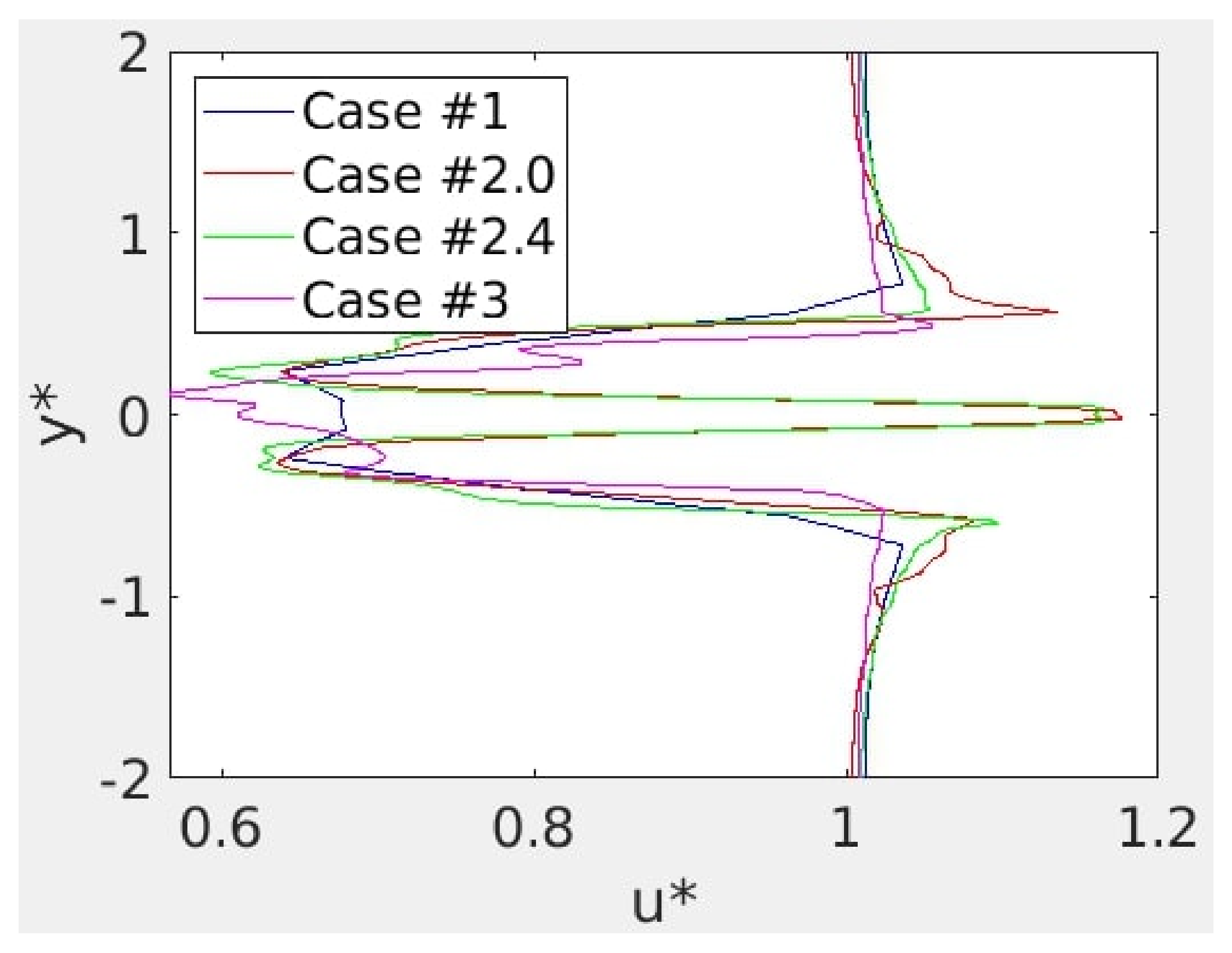
Figure 14.
Same legend as previous one but for = 2.
Figure 14.
Same legend as previous one but for = 2.
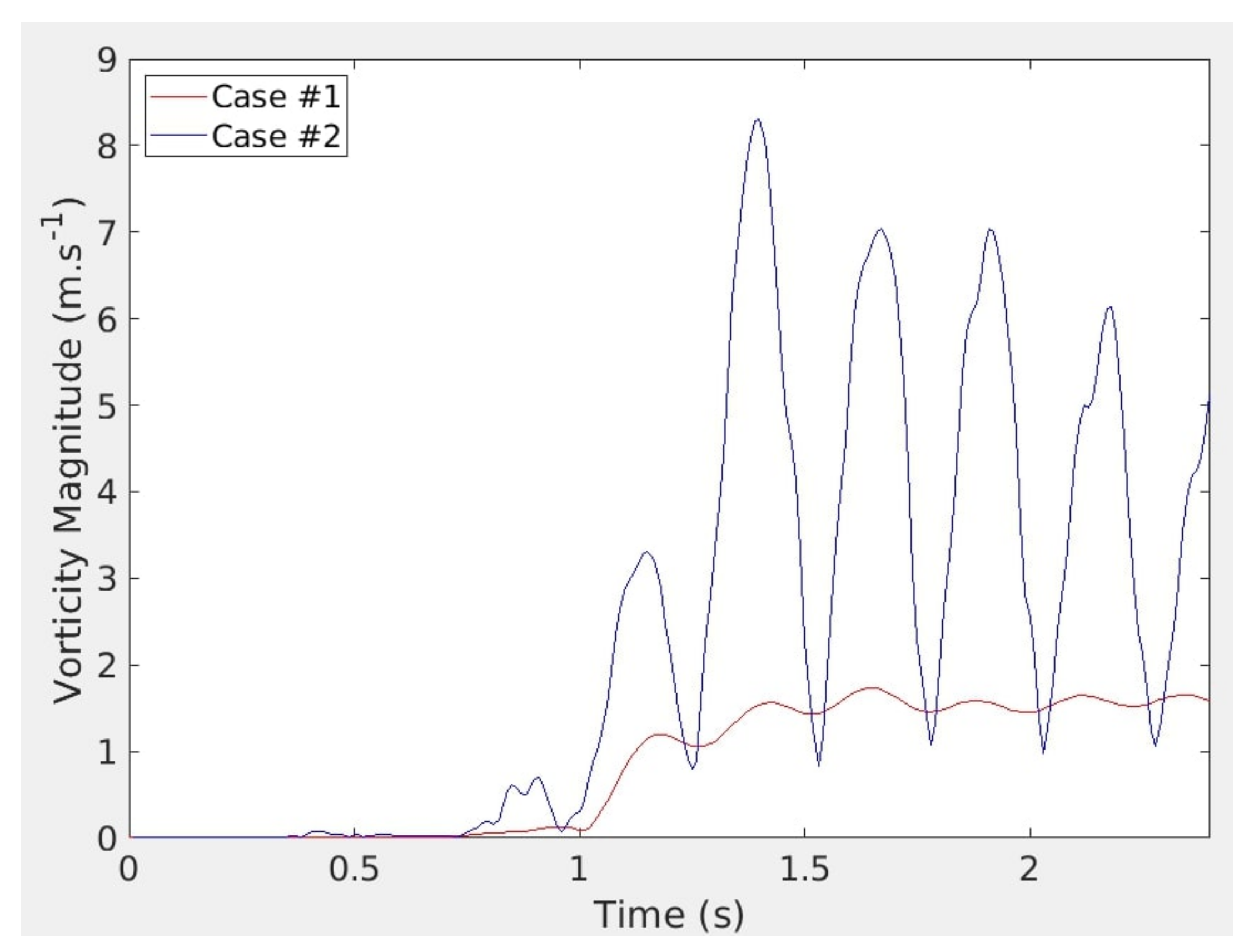
Figure 15.
Time evolution of the vorticity magnitude close to the rotor, inside the AMI zone ( = 2), for coarse (#1 with red line) and refined (#2 with blue line) meshes.
Figure 15.
Time evolution of the vorticity magnitude close to the rotor, inside the AMI zone ( = 2), for coarse (#1 with red line) and refined (#2 with blue line) meshes.
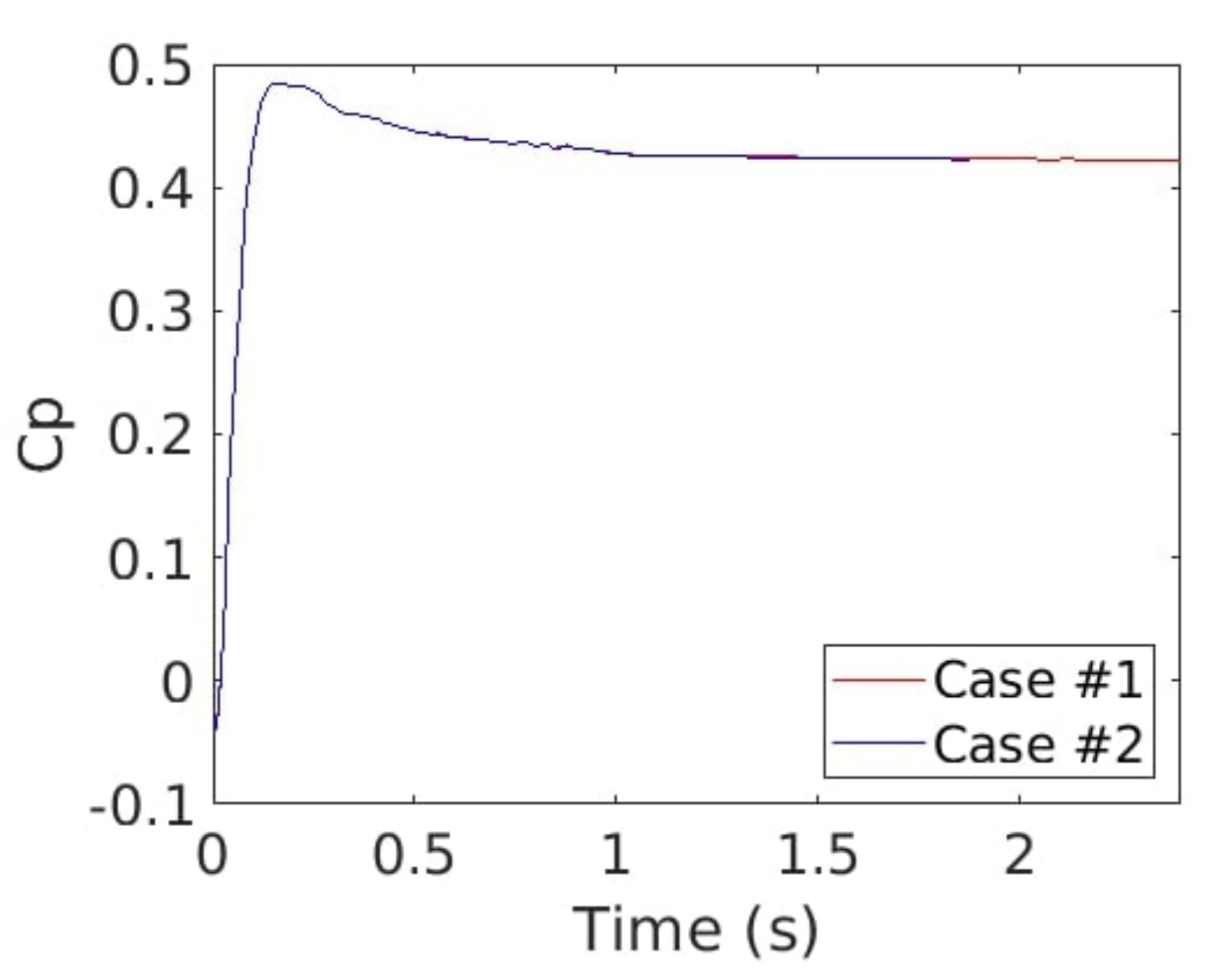
Figure 16.
Time evolution of the power coefficient (Cp) with coarse (red line) and fine (blue line) mesh refinement in the wake.
Figure 16.
Time evolution of the power coefficient (Cp) with coarse (red line) and fine (blue line) mesh refinement in the wake.
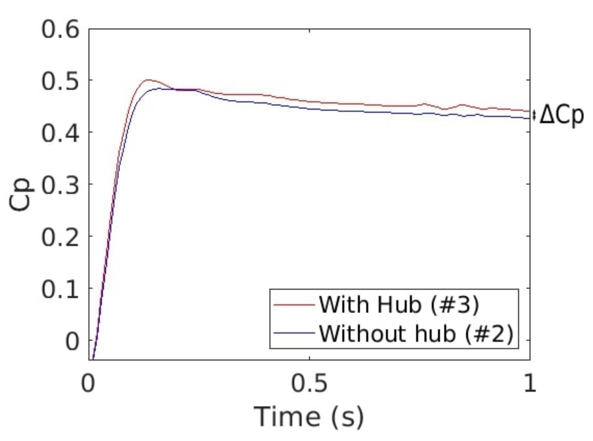
Figure 17.
Time evolution of Cp for the cases with (#3 red line) and without a hub (#2.0 blue line).
Figure 17.
Time evolution of Cp for the cases with (#3 red line) and without a hub (#2.0 blue line).
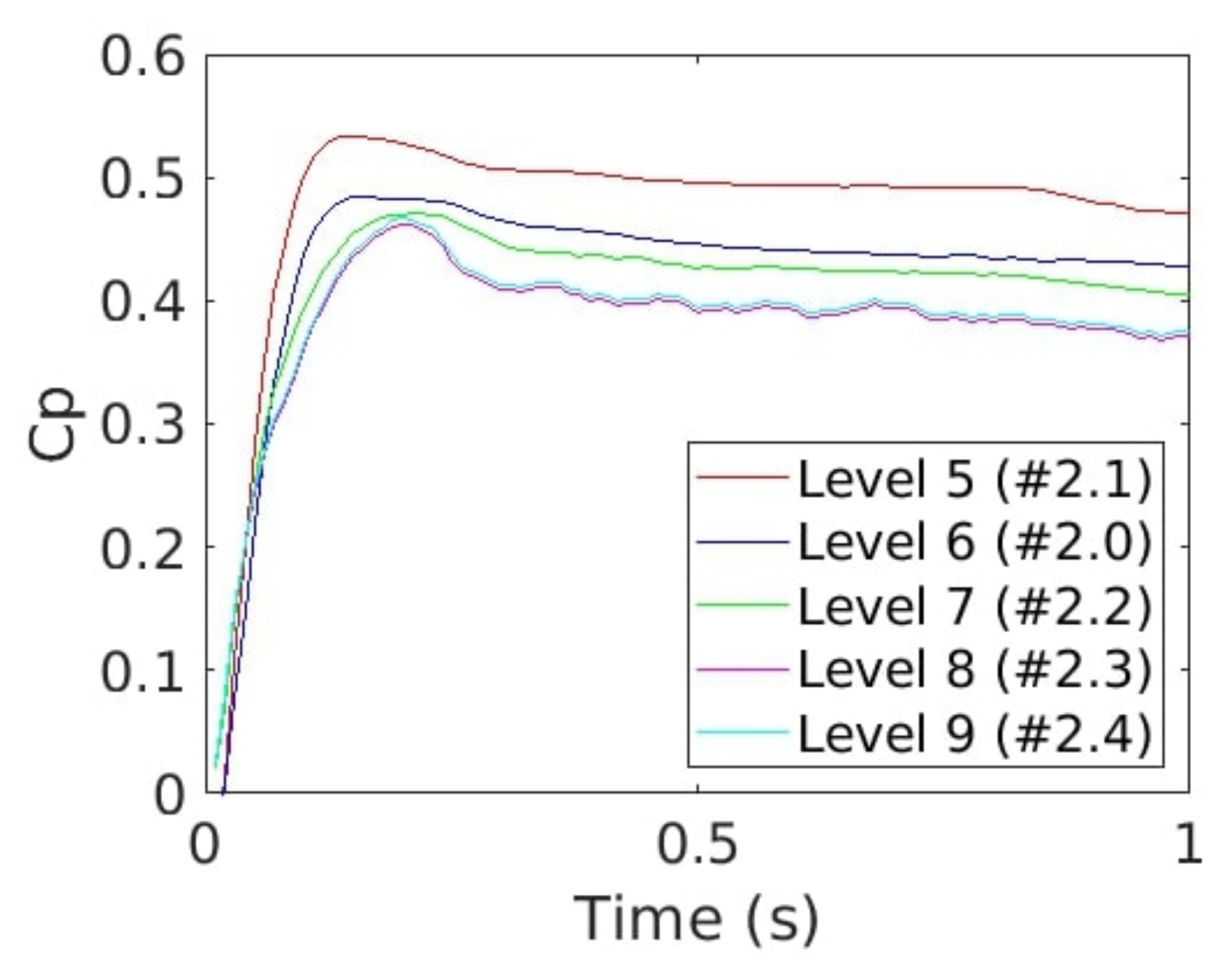
Figure 18.
Cp time evolution for cases #2.0 (blue), #2.1 (red), #2.2 (green), #2.3 (pink) and #2.4 (cyan).
Figure 18.
Cp time evolution for cases #2.0 (blue), #2.1 (red), #2.2 (green), #2.3 (pink) and #2.4 (cyan).
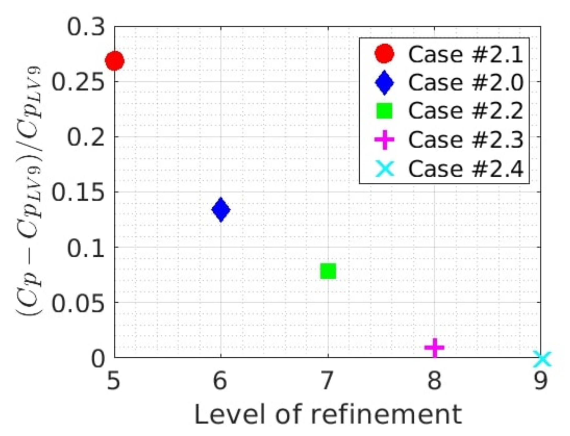
Figure 19.
Relative difference between Cp after 1 s of simulation for cases #2.0 (blue lozenge), #2.1 (red dot), #2.2 (green square), #2.3 (pink plus), #2.4 (cyan cross) and #2.4.
Figure 19.
Relative difference between Cp after 1 s of simulation for cases #2.0 (blue lozenge), #2.1 (red dot), #2.2 (green square), #2.3 (pink plus), #2.4 (cyan cross) and #2.4.
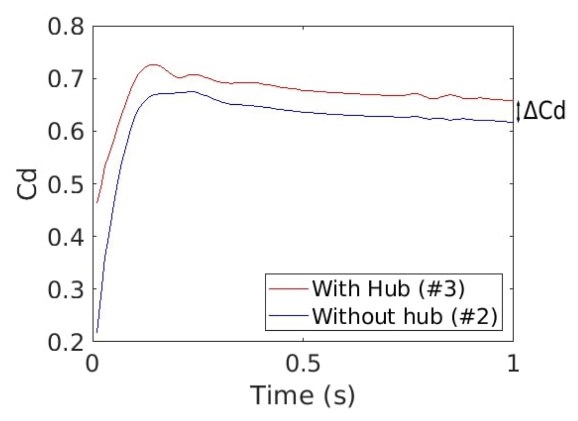
Figure 20.
time evolution for the cases with (#3) and without a hub (#2.0).
Figure 20.
time evolution for the cases with (#3) and without a hub (#2.0).
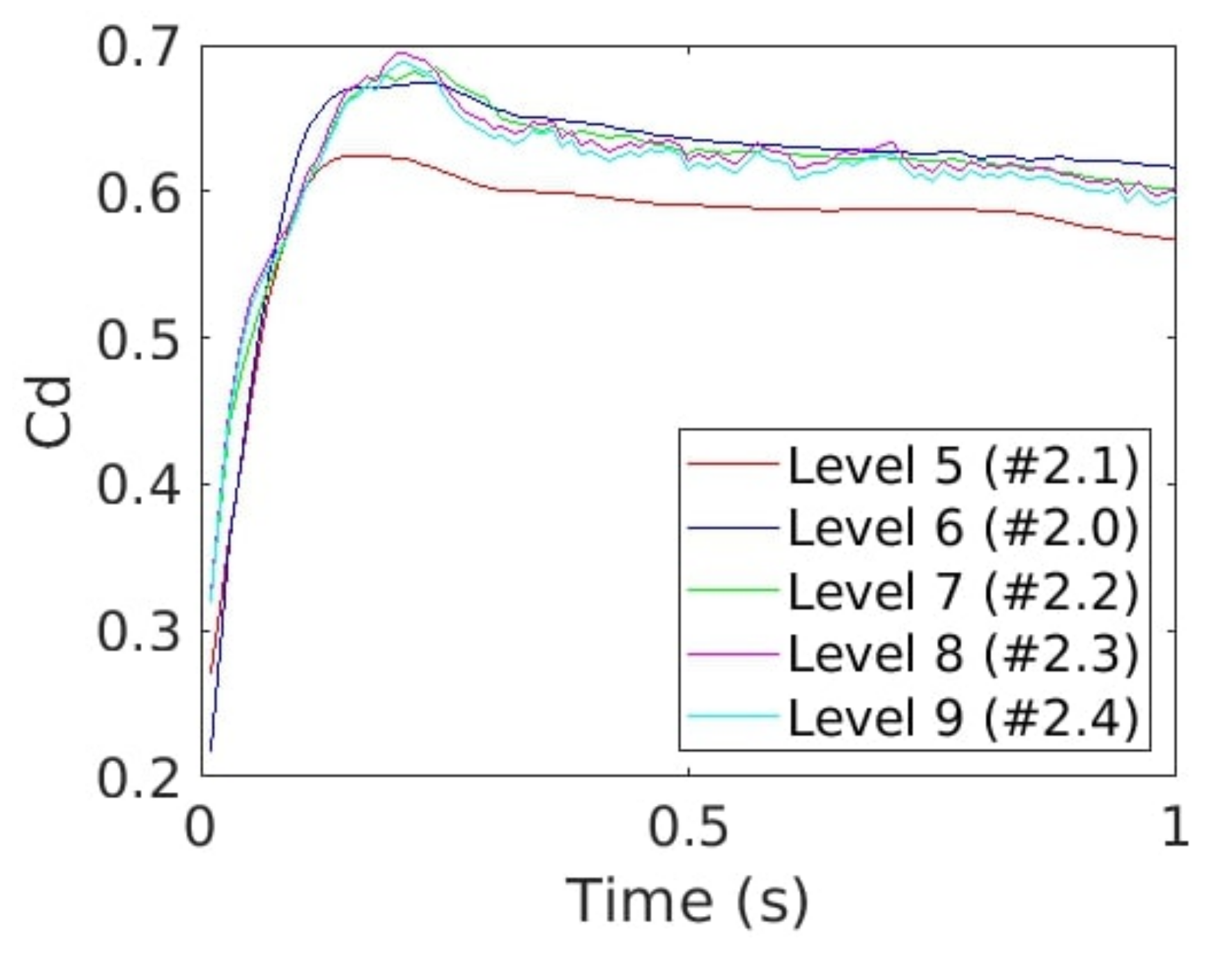
Figure 21.
time evolution according to the level of refinement for cases #2.0 (blue), #2.1 (red), #2.2 (green), #2.3 (pink) and #2.4 (cyan).
Figure 21.
time evolution according to the level of refinement for cases #2.0 (blue), #2.1 (red), #2.2 (green), #2.3 (pink) and #2.4 (cyan).
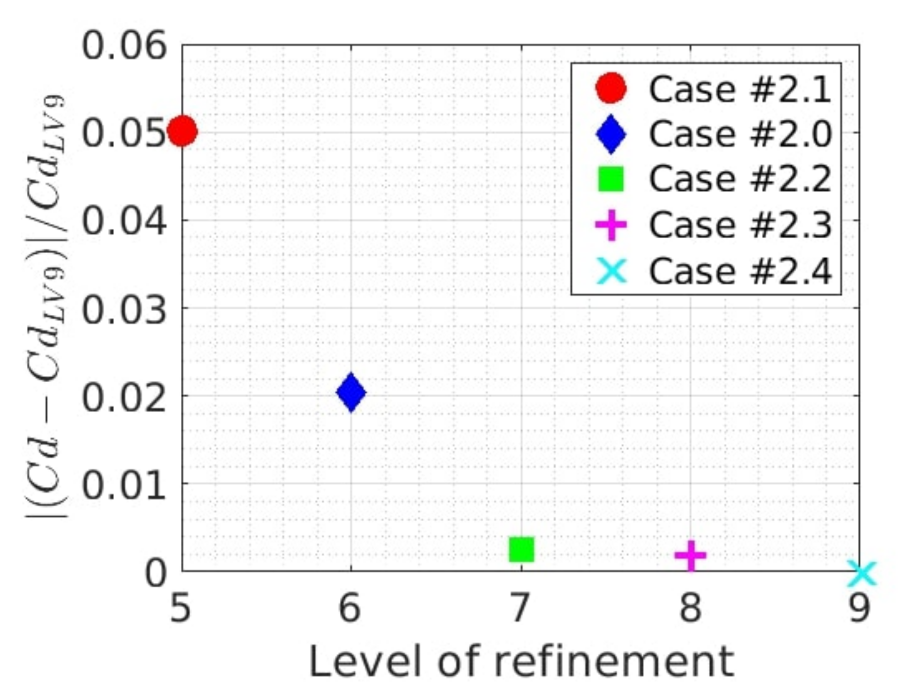
Figure 22.
Relative difference in according to the level of refinement for cases #2.0 (blue lozenge), #2.1 (red dot), #2.2 (green square), #2.3 (pink plus), #2.4 (cyan cross) and #2.4.
Figure 22.
Relative difference in according to the level of refinement for cases #2.0 (blue lozenge), #2.1 (red dot), #2.2 (green square), #2.3 (pink plus), #2.4 (cyan cross) and #2.4.
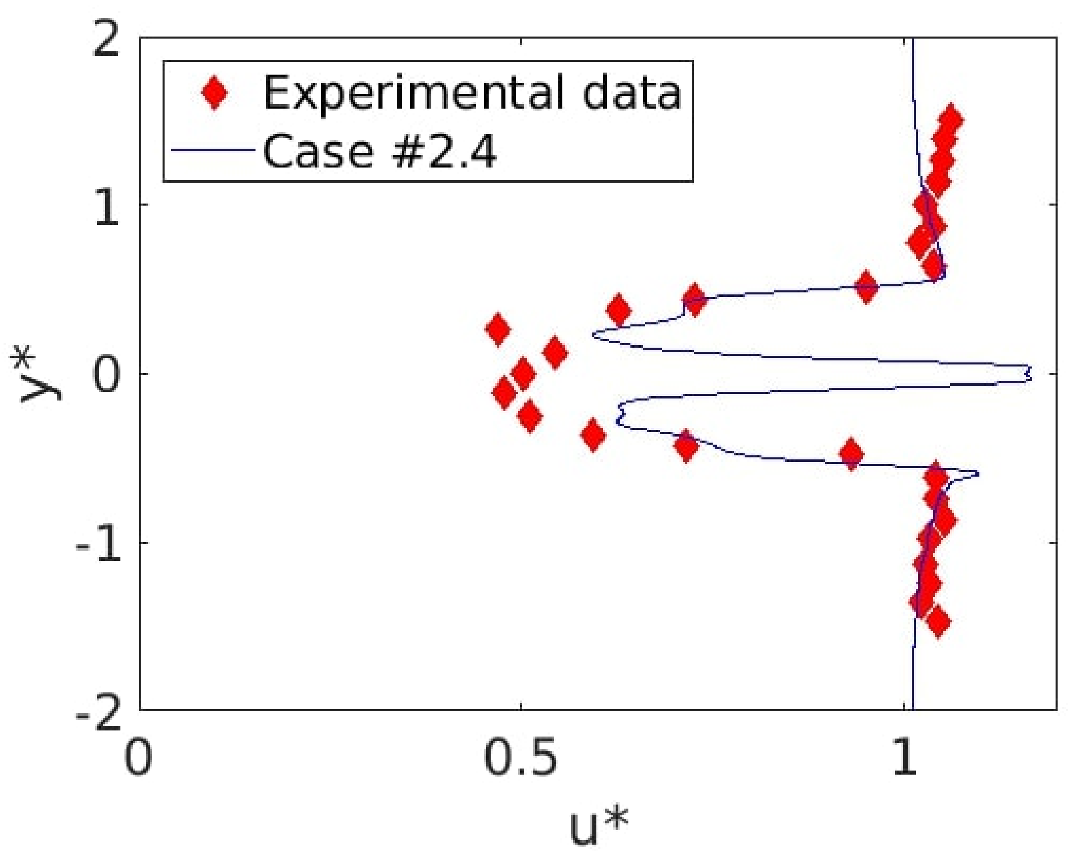
Figure 23.
Non-dimensional velocity profiles according to the non-dimensional position for experimental data (red lozenges) and model (#2.4) as . The mismatch at was due to the missing hub in the numerical case.
Figure 23.
Non-dimensional velocity profiles according to the non-dimensional position for experimental data (red lozenges) and model (#2.4) as . The mismatch at was due to the missing hub in the numerical case.
Figure 24.
Same legend as for previous figure, but profiles were taken at . The mismatch at was due to the missing hub in the numerical case.
Figure 24.
Same legend as for previous figure, but profiles were taken at . The mismatch at was due to the missing hub in the numerical case.
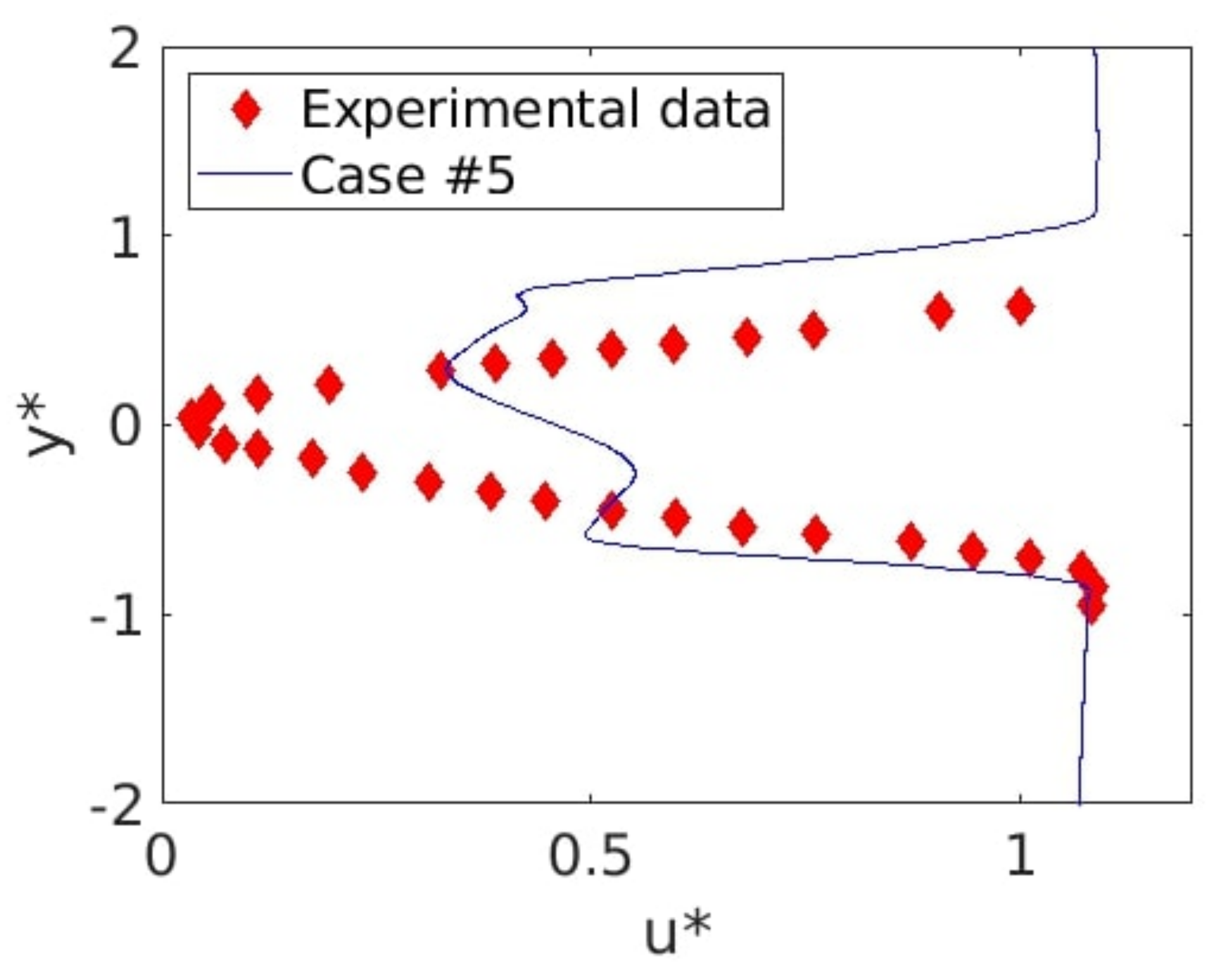
Figure 25.
depending on the position comparison between case #5 (blue line) and experimental data (red lozenges) at .
Figure 25.
depending on the position comparison between case #5 (blue line) and experimental data (red lozenges) at .
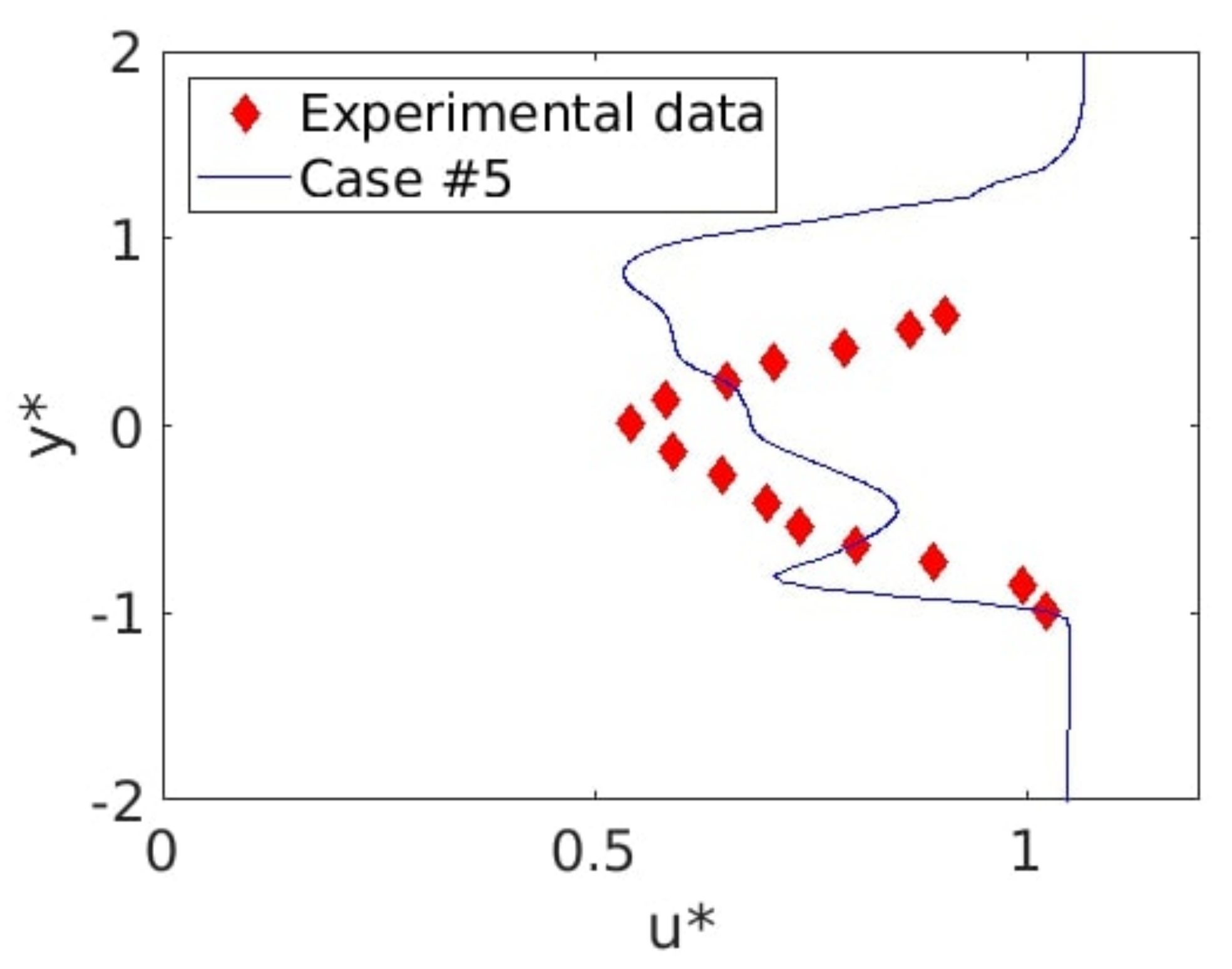
Figure 26.
depending on the position comparison between case #5 (blue line) and experimental data (red lozenges) at .
Figure 26.
depending on the position comparison between case #5 (blue line) and experimental data (red lozenges) at .
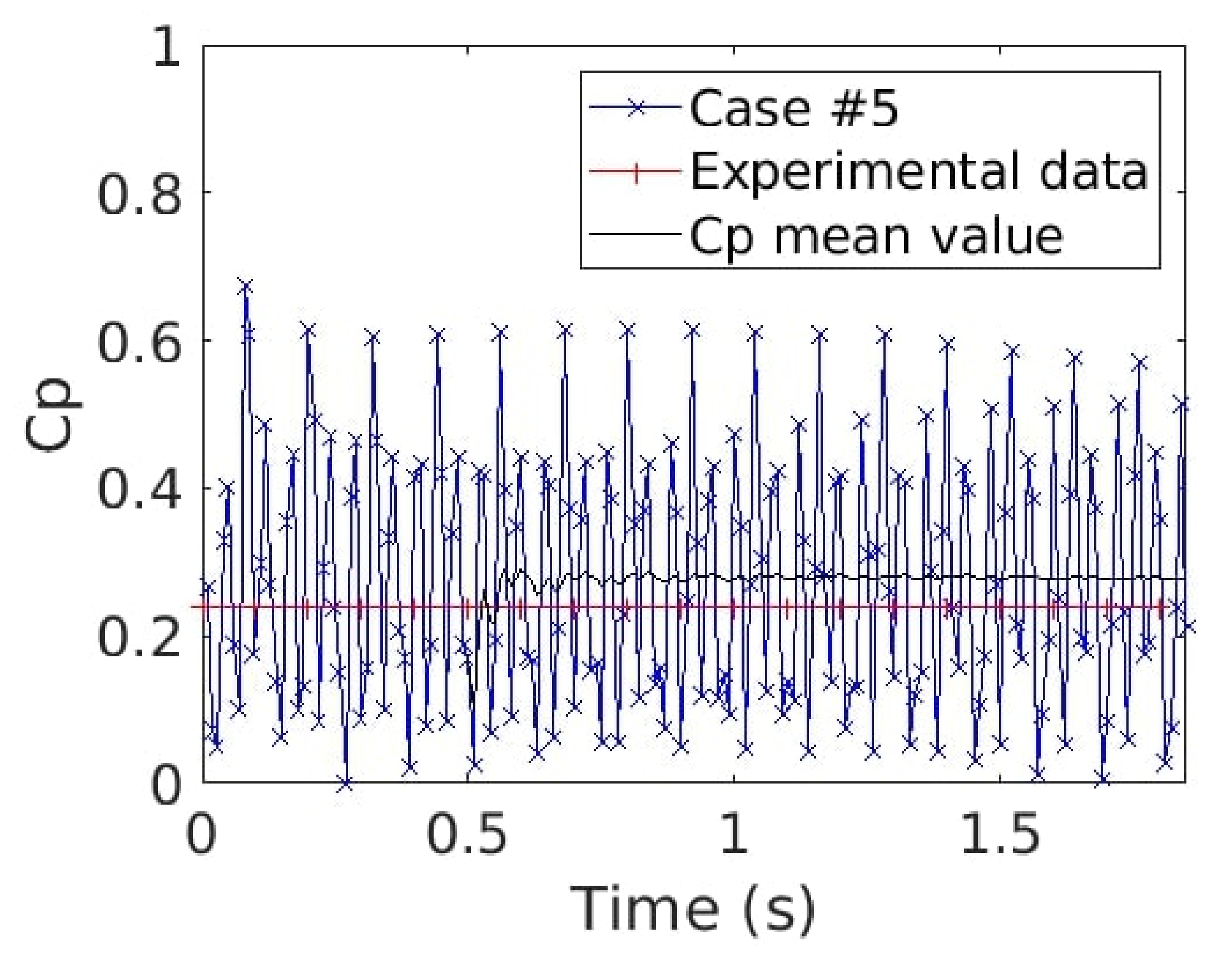
Figure 27.
Time evolution of the power coefficient Cp for case #5 (blue line with crosses) and experimental data (red line with plus). The black line is the Cp mean value starting at 0.5 s.
Figure 27.
Time evolution of the power coefficient Cp for case #5 (blue line with crosses) and experimental data (red line with plus). The black line is the Cp mean value starting at 0.5 s.
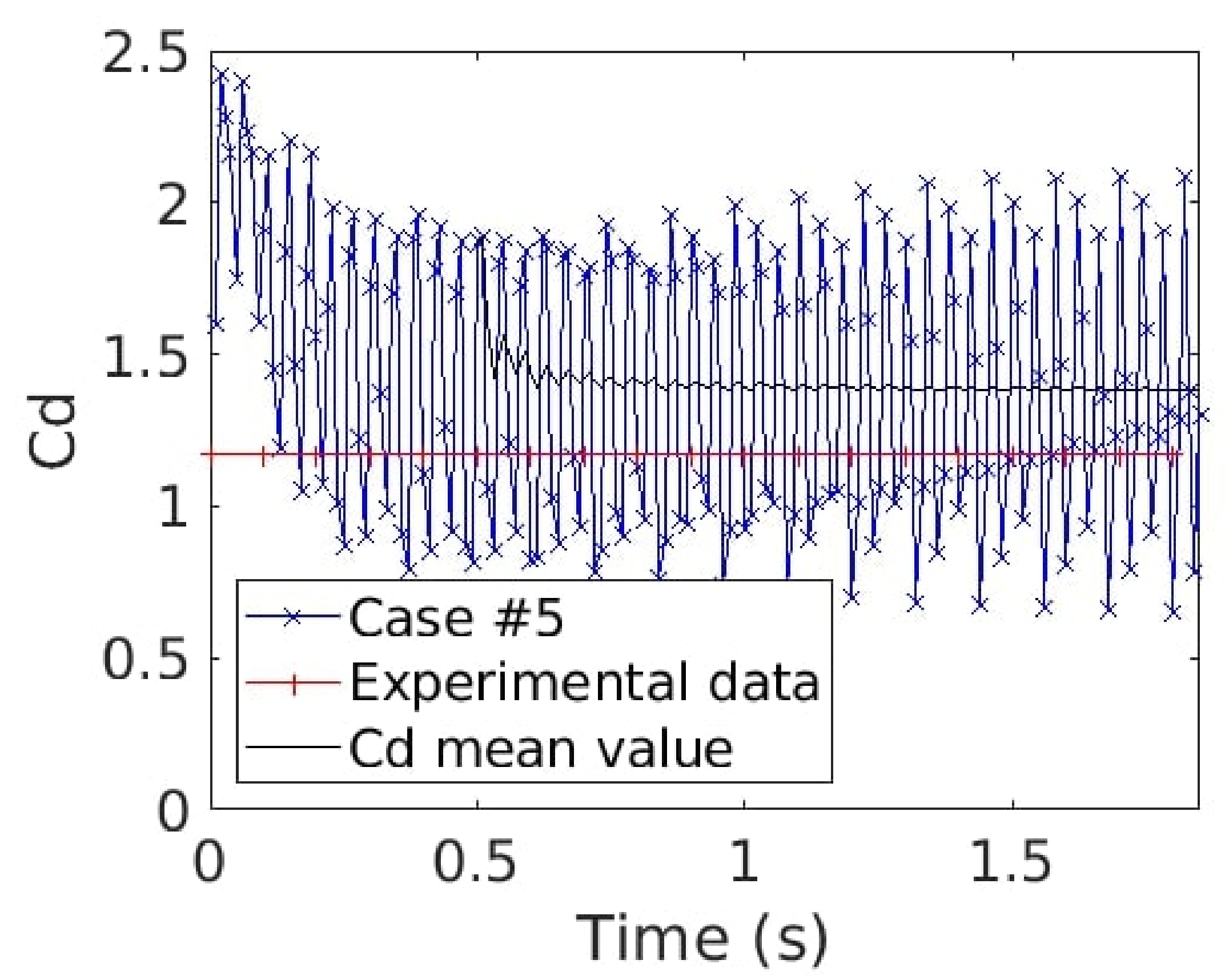
Figure 28.
Time evolution of the drag coefficient for case #5 (blue line with crosses) and experimental data (red line with plus). The black line is the Cp mean value starting at 0.5 s.
Figure 28.
Time evolution of the drag coefficient for case #5 (blue line with crosses) and experimental data (red line with plus). The black line is the Cp mean value starting at 0.5 s.
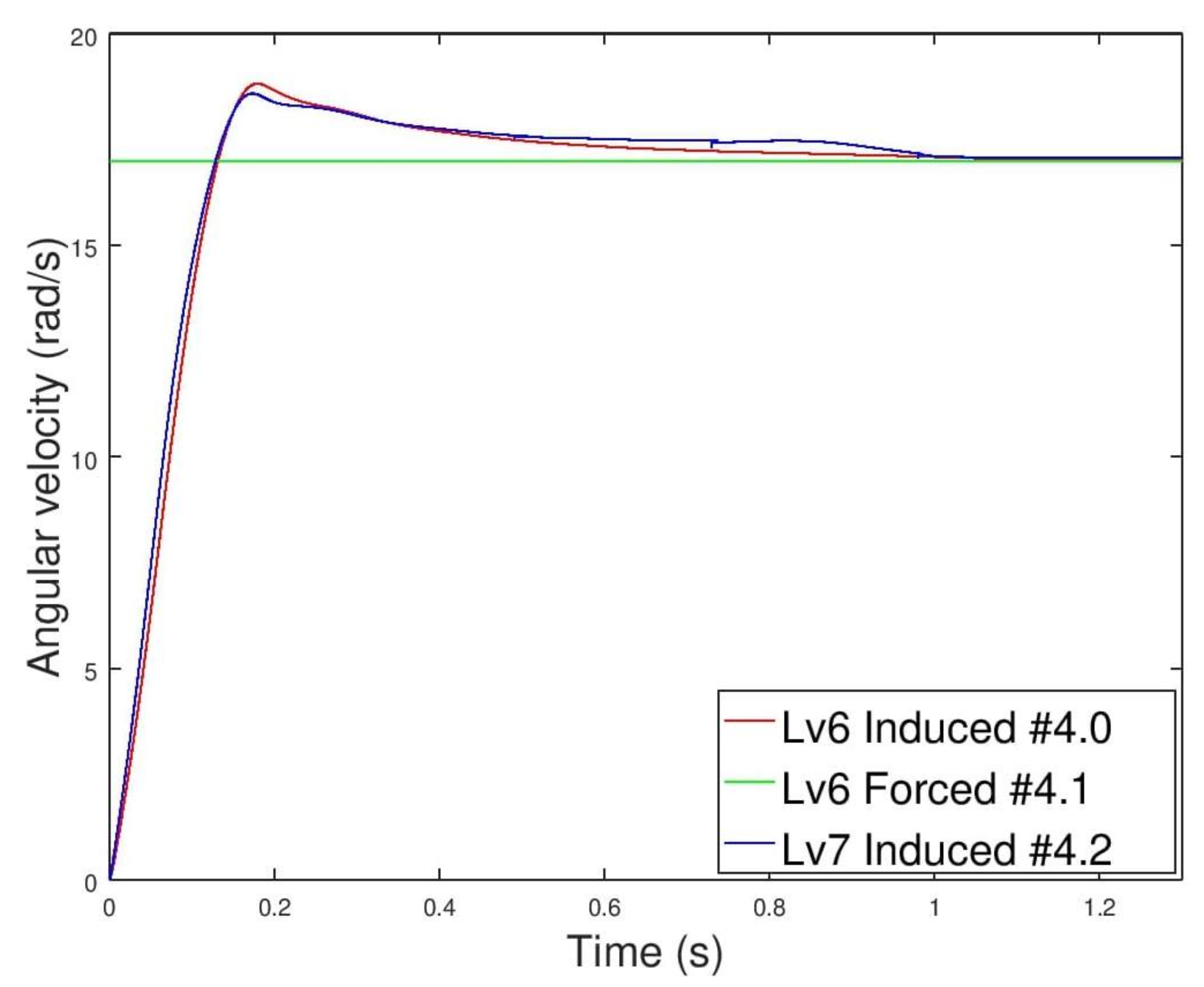
Figure 29.
Time evolution of the angular velocity for cases #4.0 (red line), #4.1 (green line) and #4.2 (blue line).
Figure 29.
Time evolution of the angular velocity for cases #4.0 (red line), #4.1 (green line) and #4.2 (blue line).
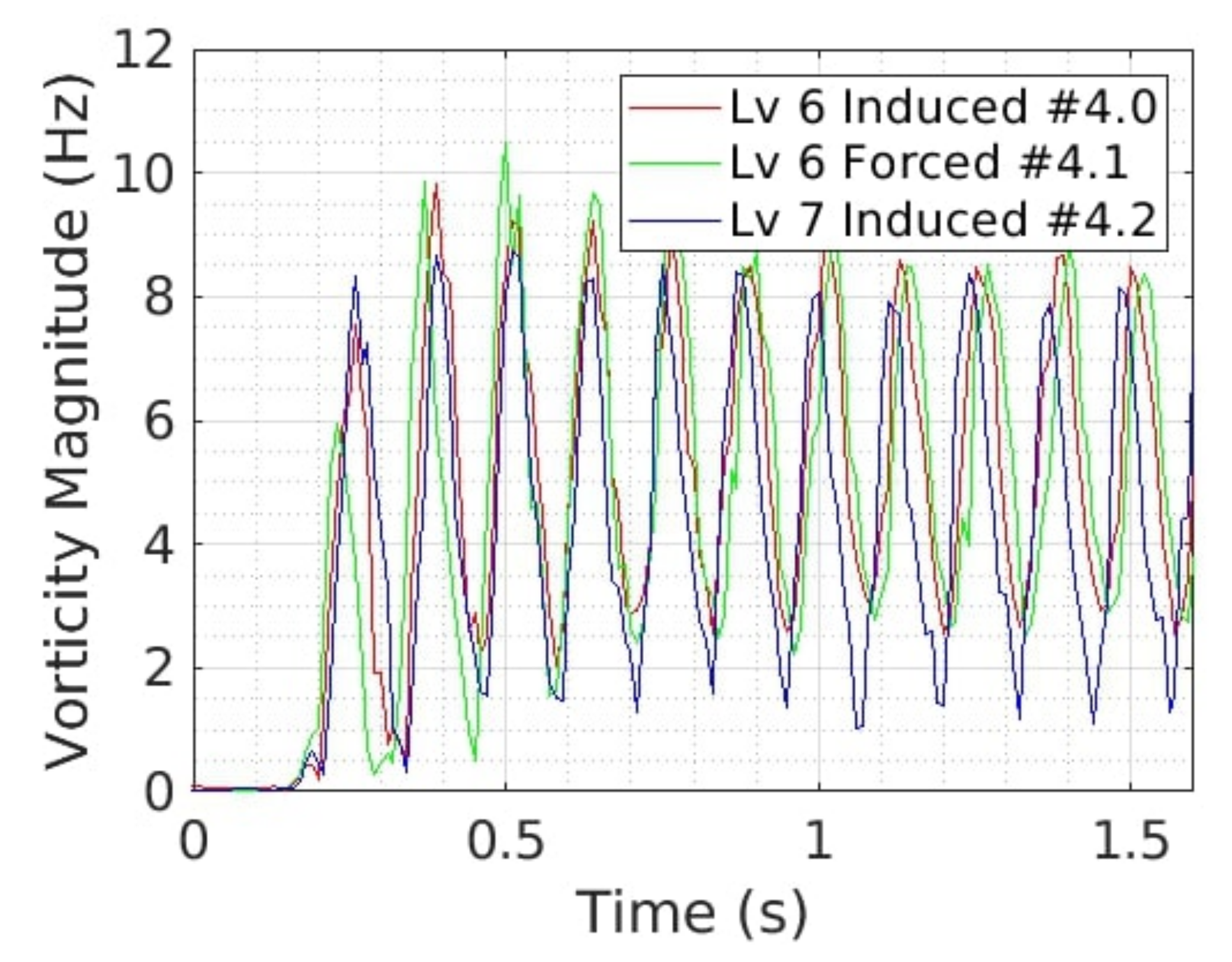
Figure 30.
Time evolution of the vorticity magnitude at the probe position (, ) after phase shift correction for #4.0 (red line), #4.1 (green line) and #4.2 (blue line).
Figure 30.
Time evolution of the vorticity magnitude at the probe position (, ) after phase shift correction for #4.0 (red line), #4.1 (green line) and #4.2 (blue line).
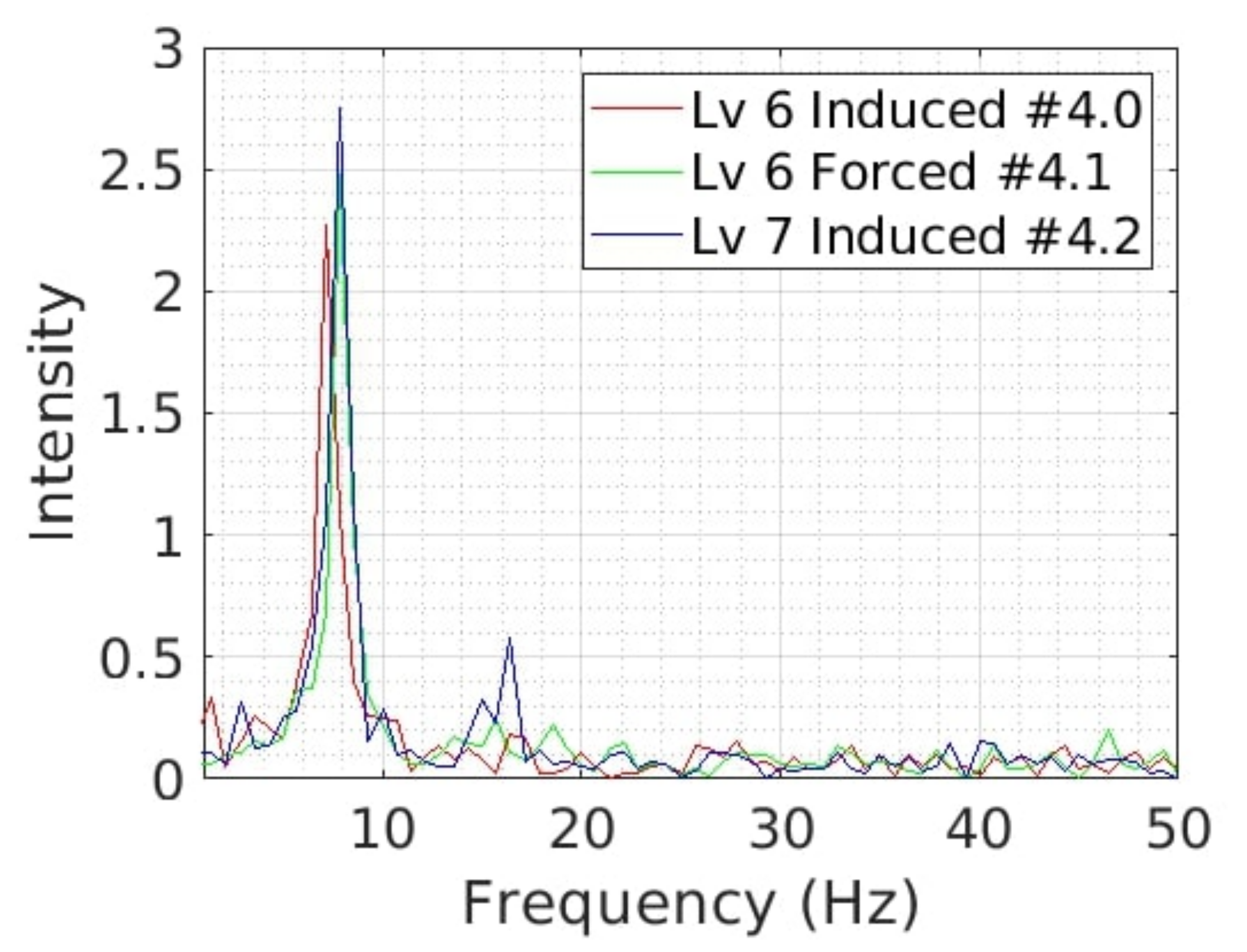
Figure 31.
Frequency-based spectra of vorticity for the cases #4.0 (red line), #4.1 (green line) and #4.2 (blue line).
Figure 31.
Frequency-based spectra of vorticity for the cases #4.0 (red line), #4.1 (green line) and #4.2 (blue line).
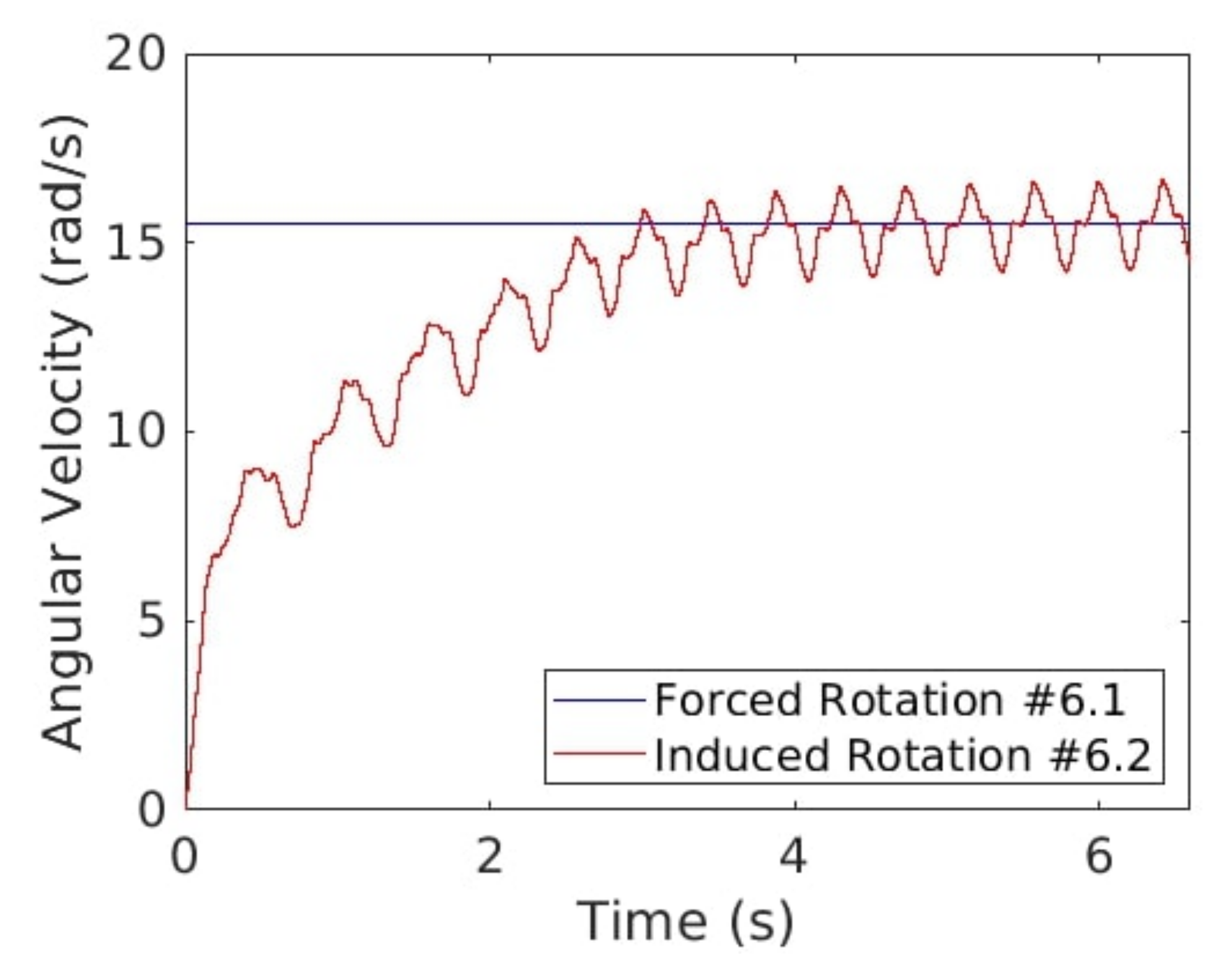
Figure 32.
Time evolution of the angular velocity for forced (blue line, #6.1) and induced (red line, #6.2) rotation.
Figure 32.
Time evolution of the angular velocity for forced (blue line, #6.1) and induced (red line, #6.2) rotation.
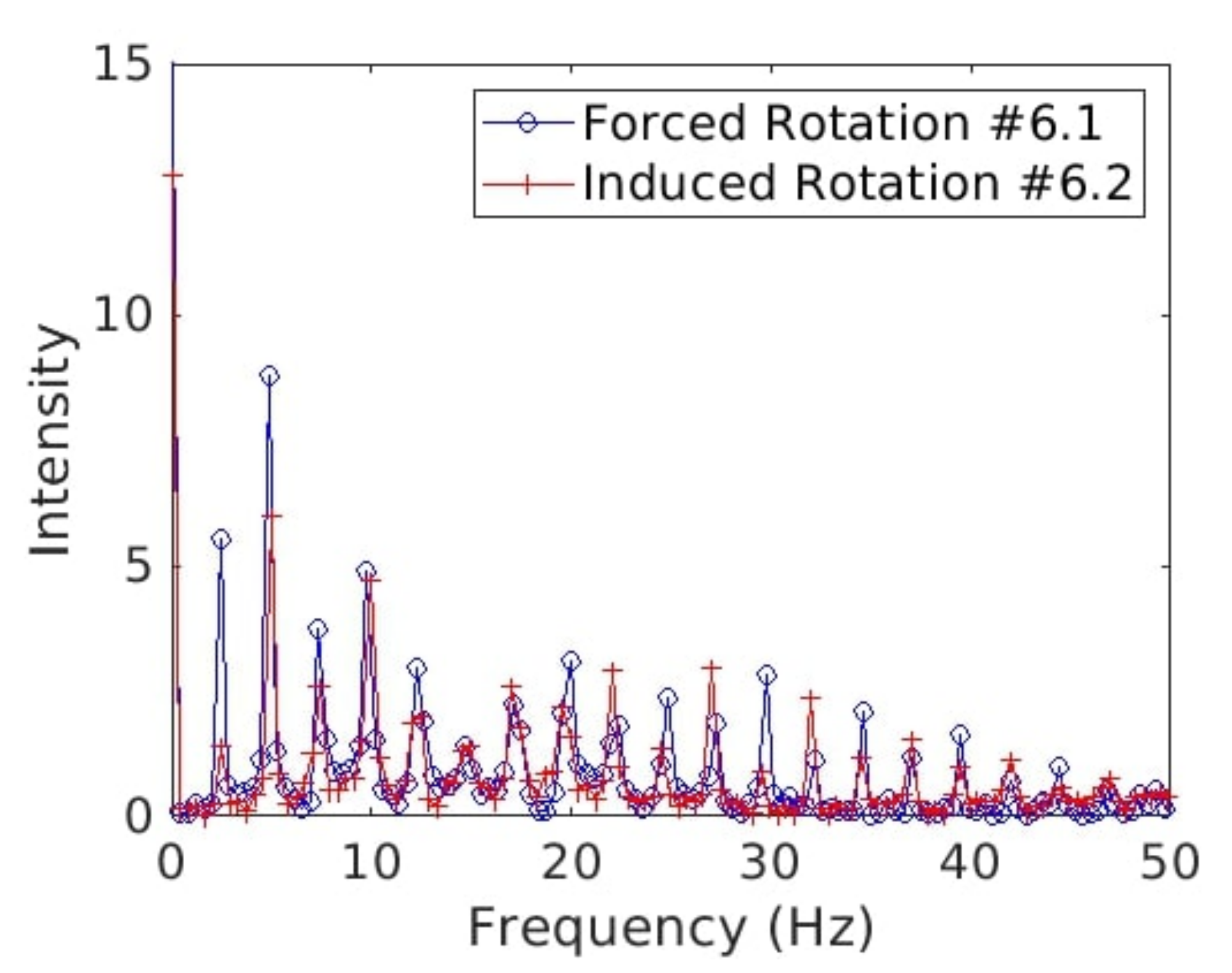
Figure 33.
Frequency-based spectra of the vorticity for forced (blue line, #6.1) and induced (red line, #6.2) rotation cases.
Figure 33.
Frequency-based spectra of the vorticity for forced (blue line, #6.1) and induced (red line, #6.2) rotation cases.
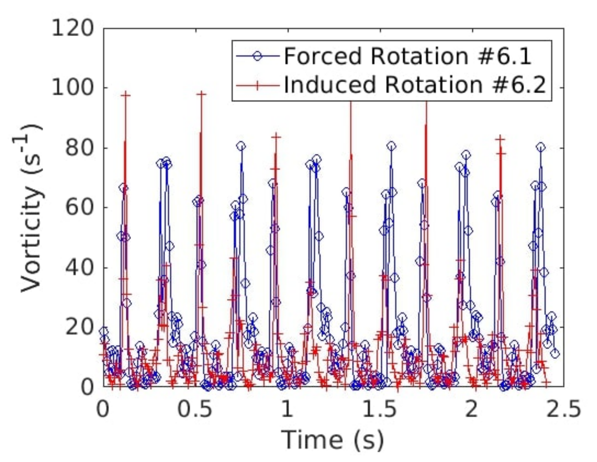
Figure 34.
Time evolution of the fluid vorticity at the probe location for forced (blue line, #6.1) and induced (red line, #6.2) rotation.
Figure 34.
Time evolution of the fluid vorticity at the probe location for forced (blue line, #6.1) and induced (red line, #6.2) rotation.
Table 1.
Summary of the characteristic lengths of the cells relative to the levels of refinement.
Table 1.
Summary of the characteristic lengths of the cells relative to the levels of refinement.
| Levels | Characteristic Length |
|---|
| Level 1 | |
| Level 2 | |
| Level 3 | |
| Level 4 | |
| Level 5 | |
| Level 6 | |
| Level 7 | |
| Level 8 | |
| Level 9 | |
Table 2.
Summary of test cases for the horizontal axis turbine according to the level of refinement on the blades and in the wake, the presence or absence of a hub, and the total number of points in the mesh (Nb).
Table 2.
Summary of test cases for the horizontal axis turbine according to the level of refinement on the blades and in the wake, the presence or absence of a hub, and the total number of points in the mesh (Nb).
| Mesh | Level on Blades | Level in Wake | Hub | Nb () |
|---|
| Reference case (#1) | Level 6 | Level 1 | No | 1 |
| Wake case (#2.0) | Level 6 | Level 3 | No | 1.9 |
| Blade 5 (#2.1) | Level 5 | Level 3 | No | 1.6 |
| Blade 7 (#2.2) | Level 7 | Level 3 | No | 3.5 |
| Blade 8 (#2.3) | Level 8 | Level 3 | No | 9 |
| Blade 9 (#2.4) | Level 9 | Level 3 | No | 12 |
| Hub case (#3) | Level 6 | Level 3 | Yes | 2.2 |
| Flow-induced L6 (#4.0) | Level 6 | Level 3 | No | 1.9 |
| Forced free rotation speed L6 (#4.1) | Level 6 | Level 3 | No | 1.9 |
| Flow-induced L7 (#4.2) | Level 7 | Level 3 | No | 3.5 |
Table 3.
Summary of test cases for vertical axis turbine according to the level of refinement on the blades and in the wake, the presence or absence of a hub, and the total number of points in the mesh (Nb).
Table 3.
Summary of test cases for vertical axis turbine according to the level of refinement on the blades and in the wake, the presence or absence of a hub, and the total number of points in the mesh (Nb).
| Mesh | Level on Blades | Level in Wake | Hub | Nb () |
|---|
| Forced for validation (#5) | Level 6 | Level 3 | No | 1.2 |
| Forced free speed (#6.1) | Level 6 | Level 3 | No | 1.2 |
| Flow induced (#6.2) | Level 6 | Level 3 | No | 1.2 |
Table 4.
Table of the physical parameters used in simulations for horizontal and vertical axis cases.
Table 4.
Table of the physical parameters used in simulations for horizontal and vertical axis cases.
| Parameter | Horizontal Axis Turbine | Vertical Axis Turbine | Unit |
|---|
| 1025 | 998 | |
| | | |
| | | |
| | | |
| 4 | 2 | - |
Table 5.
Summary of the Cp values after 1 s of simulation depending on the level of refinement on the blades. The relative difference compared to the level 9 simulation is given in the last column.
Table 5.
Summary of the Cp values after 1 s of simulation depending on the level of refinement on the blades. The relative difference compared to the level 9 simulation is given in the last column.
| Level | Case | Cp | Relative Difference |
|---|
| 5 | #2.1 | | 0.2688 |
| 6 | #2.0 | | 0.1341 |
| 7 | #2.2 | | 0.0787 |
| 8 | #2.3 | | 0.0095 |
| 9 | #2.4 | | 0 |
Table 6.
Summary of the Cd values after 1 s of simulation depending on the level of refinement on the blades. The relative difference compared to the level 9 simulation is given in the last column.
Table 6.
Summary of the Cd values after 1 s of simulation depending on the level of refinement on the blades. The relative difference compared to the level 9 simulation is given in the last column.
| Level | Case | Cd | Relative Difference |
|---|
| 5 | #2.1 | 0.5698 | 0.0501 |
| 6 | #2.0 | 0.6120 | 0.0.0203 |
| 7 | #2.2 | | 0.0025 |
| 8 | #2.3 | | 0.0020 |
| 9 | #2.4 | | 0 |
Table 7.
Coefficient values with their relative differences with the experiment data.
Table 7.
Coefficient values with their relative differences with the experiment data.
| Coefficient | Value | Relative Difference |
|---|
| 0.3729 | 0.070 |
| 0.3887 | 0.031 |
| 0.5998 | 0.1552 |
| 0.6418 | 0.09 |
Table 8.
Coefficient values with their relative differences with the experiment data.
Table 8.
Coefficient values with their relative differences with the experiment data.
| Coefficient | Experimental | Numerical | Relative Difference |
|---|
| 0.24 | 0.2779 | 0.1576 |
| 1.13 | 1.3806 | 0.1800 |


