Imbalance Fault Classification Based on VMD Denoising and S-LDA for Variable-Speed Marine Current Turbine

Abstract

Marine current energy as a kind of renewable energy has gradually attracted more and more attention from many countries. However, the blade imbalance fault of marine current turbines (MCTs) will have an effect on the power production efficiency and cause damage to the MCT system. It is hard to classify the severity of an MCT blade imbalance fault under the condition of the current instability and seafloor noise. This paper proposes a fault classification method based on the combination of variational mode decomposition denoising (VMD denoising) and screening linear discriminant analysis (S-LDA). The proposed method consists of three parts. Firstly, phase demodulation of the collected stator current signal is performed by the Hilbert transform (HT) method. Then, the obtained demodulation signal is denoised by variational mode decomposition denoising (VMD denoising), and the denoised signal is analyzed by power spectral density (PSD). Finally, S-LDA is employed on the power signal to determine the severities of fault classification. The effectiveness of the proposed method is verified by experimental results under different severities of blade imbalance fault. The stator current signatures of experiments with different severities of blade imbalance fault are used to validate the effectiveness of the proposed method. The fault classification accuracy is 92.04% based on the proposed method. Moreover, the experimental results verify that the influence of velocity fluctuation on fault classification can be eliminated.

1. Introduction

Marine current energy has been developed for several decades around the world [1,2,3]. However, marine current turbines (MCTs) are easily broken down because they are commonly installed in a harsh marine environment. When an MCT works on the seafloor for a long time, the blades are easily attached to by marine organisms [4,5,6], which may cause blade imbalance fault. Therefore, the generating efficiency of the marine energy conversion system (MECS) will be decreased and the lifetime of the MECS will be shortened as the fault reaches a certain degree. Moreover, the blade fault could lead to a rotor eccentricity fault. For a fixed-pitch MCT, an eccentricity fault less than 10% can be ignored, and an eccentricity fault greater than 60% needs to be repaired immediately in order to prevent friction between the stator and the center from damaging the machine [7]. Therefore, it is of great significance for the normal operation of the unit and the avoidance of greater damage to classify the severities of blade imbalance faults.

The faults in an MECS commonly include blade imbalance, bearing, and eccentricity. For the faults mentioned above, sensors are needed to collect signals for fault detection and diagnosis [8,9,10,11,12]. Xie et al. [12] reviewed different blade fault types under the condition of turbulence and current blade fault detection methods, and the signal used for fault detection in MCTs was also explained. In [13,14,15,16,17,18,19], vibration signals were obtained by a vibration sensor to detect motor bearing faults. A Hall sensor is used to detect the bearing faults of a motor in [20]. The fault detection method was also applied based on the motor speed signature [21]. Image signals obtained by an underwater camera were used to detect blade imbalance fault in an MCT in [22,23]. However, these sensors need to be waterproof and compression-resistant, which are difficult to install under complex conditions. The current sensor is free of exposure to the complex environment [24].

Therefore, fault detection and diagnosis based on electrical signals is a good choice for MCTs. There are many fault detection studies where power signals or modular square signals are used to detect faults [25,26]. However, the power signal is calculated from the voltage and current signal, and the mode square signal is obtained by the three-phase electrical signal. The use of a power signal or modular square signal will increase the sample set and the risk of failure detection due to sensor failure. Therefore, in order to avoid this problem, single-phase electrical signals are applied in the proposed method. Since many faults lead to phase modulation of electrical signals, many fault detection methods are based on frequency demodulation of electrical signals to obtain fault characteristics [27,28]. In [27], the Least Squares Estimator (LSE) is used to demodulate the corresponding amplitudes of stator current signals. A fault severity criterion which is derived from the amplitude estimates is applied to make a classification for bearing and broken rotor bar faults. In [28], the frequency of stator current is estimated based on a modified version of multiple signal classification (MUSIC). In [29,30,31], the Hilbert transform (HT) is applied to demodulate electrical signals. In [30], the instantaneous frequency of the voltage signal is obtained by the Hilbert transform, and the angular frequency and complex phasors are obtained by the maximum likelihood estimator in [31]. However, the above papers do not take into account the influence of the non-stationary conditions.

Some scholars take advantage of the decomposition method’s characteristics for denoising to eliminate the influence of the wave and turbulence. In [32], Li proposed another strategy of fault detection. The current signal is denoised by wavelet threshold denoising. Then, the Hilbert transform is applied to demodulate. Finally, the imbalance fault is detected by the computation of statistics indices in the principal and residual subspaces of principal component analysis (PCA) under different fixed flow conditions. In [33,34,35,36], the proposed method is used to denoise based on empirical mode decomposition (EMD). The methods mentioned above are applied to detect the blade imbalance fault of an MCT, such as EMD and wavelet transform (WT). However, these methods have shortcomings. For example, EMD has some disadvantages such as mode mixing, end effect, and sensitivity to sampling, which can affect fault detection. Moreover, the selection of wavelet bases in WT is difficult. When an MCT operates under different working conditions, the appropriate wavelet basis may be selected differently, which will lead to low robustness of fault detection. In addition to the decomposition method, the resampling method is also used to deal with non-stationary conditions. In [37], a new adaptive proportional sampling frequency (APSF) is applied to transform the variable fault features into fixed ones. However, although the methods mentioned above can detect imbalance faults based on electrical signals, they cannot be used to make fault classifications for MCTs.

In [38], a 1D convolutional neural network is used to extract features and fault classification for rub-impact. However, the effect of the non-stationary conditions is not eliminated by the above two methods. In [39], the fault feature is obtained by a continuous Morlet wavelet transform (CMWT). Secondly, principal component analysis (PCA) is employed to reduce the dimension. Finally, a K-nearest neighbor (KNN) machine learning algorithm is utilized to make the severity classification for rotor blade pitch imbalance faults. The main difference between this paper and the reference [39] is that the generator power signal is used in this method. Therefore, the stator current and stator voltage signals are required, which increases the sample set and the risk of failure detection due to sensor failure. In this paper, linear discriminant analysis (LDA) as a supervised dimension reduction method is more conducive to the classification of data in the later stage than PCA. The improved LDA method increases the pre-screening of the data, increases the processing efficiency of the data, and reduces the influence of useless information on the detection results. The problem of the non-stationary conditions is taken into account, but it is for the simulation signal in [39]. The actual signal of the MCT will be more complex, so it is more challenging to make fault classifications based on the actual signal.

Although the influence of variable speed is taken into account in the above papers, the severities of the imbalance faults are not classified. The single-phase current signal is utilized to avoid the situation where the signal cannot be used because of the fault of one of the current sensors based on this proposed method. In this paper, a fault classification method of blade imbalance based on the current signal is proposed under the fluctuation of velocity conditions. Firstly, HT is applied to obtain the instantaneous frequency of the single-phase stator current. Secondly, the instantaneous frequency is denoised by VMD denoising to eliminate the effects of ocean noise. Finally, screening linear discriminant analysis (S-LDA) is applied to classify the severities of imbalance faults based on the obtained passband signal power by power spectral density (PSD). The proposed method can not only detect a fault but also classify the fault effectively under the fluctuation of velocity conditions.

The rest of the paper is organized as follows. In Section 2, the problems of fault detection and diagnosis for an MCT are described. In Section 3, the proposed method for imbalance fault classification is described. In Section 4, the validity of the proposed method is shown by experimental results. Finally, the conclusion is given in Section 5.

2. Problem Description

2.1. Effect of Variable Marine Current

Under the influence of normal waves, the marine current speed can be regarded as constant. However, the marine current speed fluctuates under spring tides or strong sea conditions [40]. The current speed can be expressed by the following [41]:

$$V=V_n+\frac{\left(m-45\right)\left(V_s-V_n\right)}{95-45},$$

(1)

where $V_s$ and $V_n$ are the spring and neap tide current speed, respectively, and $m$ is the tide coefficient.

Therefore, an MCT works on variable marine current velocity, and the stator current will change with the state of flow velocity. As Figure 1 shows, as the flow velocity changes, the amplitude and frequency of the current will also change accordingly.

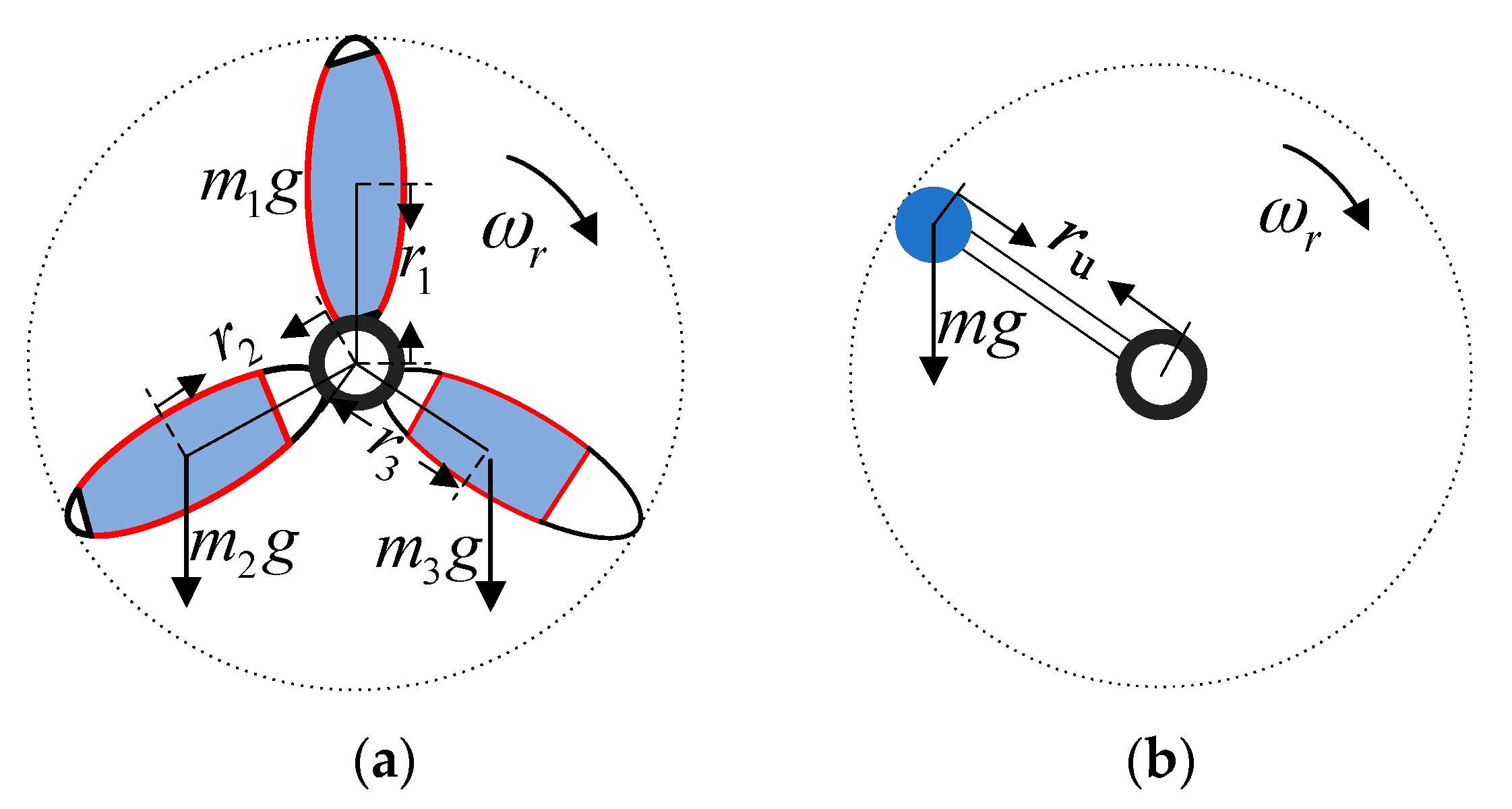
2.2. Effect of MCT Imbalance Fault

The marine current velocity will directly affect the mechanical torque of MCT. Therefore, the mechanical torque consists of two parts: the mechanical torque at a constant marine current and the additional mechanical torque under spring tides or strong sea conditions. The mechanical torque can be expressed by the following [41]:

$$T_m=T_c+T_w,$$

(2)

where $T_c$ represents mechanical torque under a constant velocity, and $T_w$ is generated by waves and turbulence [41].

As Figure 2a shows, the blades of a marine current turbine rotate at an angular velocity ${\omega }_r$, the masses of the blades are $m_1$, $m_2$, and $m_3$, and the distance from the barycenter of the blades to the hub center are $r_1$, $r_2$, and $r_3$, respectively. Assuming that the instantaneous torque of the three blades of MCT is $T_1, T_2$, and $T_3$, respectively. When the impeller is rotating, the instantaneous torque of the three blades can be expressed as the following:

$$\{\begin{array}{l}{T}_1=m_{1}g{r}_1\cos \left({\omega }_{r}t\right)\\ T_2=m_{2}g{r}_2\cos \left({\omega }_{r}t+2\pi /3\right)\\ T_3=m_{3}g{r}_3\cos \left({\omega }_{r}t-2\pi /3\right)\end{array}.$$

(3)

Then, the resultant torque can be obtained by the following:

$$\Delta T=T_1+T_2+T_3.$$

(4)

When an MCT is healthy, $\Delta T=0$. However, when an imbalance fault occurs on the blades of the MCT, $\Delta T\ne 0$. Therefore, as Figure 2b shows, the blade attachment is equivalent to a mass block with a mass of M and a distance of $r_u$ from the hub. When the blades rotate, the resultant torque also changes periodically as expressed by the following:

$$\Delta T=mg{r}_u\cos ({\omega }_{r}t+\gamma ),$$

(5)

where $\gamma$ is the initial phase.

The motion equation can be modified as:

$$J_m\frac{d{\omega }_m}{dt}=T_m+\Delta T-T_e.$$

(6)

Considering that the moment of inertia $J_m$ is large, if the imbalance fault severity of a blade is small, the electromagnetic torque $T_e\approx T_m$. Then, the actual turbine angular velocity under blade imbalance is expressed as:

$${\omega }_m={\omega }_r+\frac{mg{r}_u}{J_m\omega }\cos ({\omega }_{r}t)={\omega }_r+\Delta {\omega }_r,$$

(7)

where $\Delta {\omega }_r$ represents the change in turbine angular velocity. Therefore, the stator current can be expressed as:

$$i_A=A\cdot \sin \left(p\left({\omega }_r+\Delta {\omega }_r\right)t+\phi \right),$$

(8)

where $A$ represents the amplitude of the stator current, $p$ represents the number of pole pairs, and $\phi$ is the initial angle.

As Equations (7) and (8) show, when an MCT works under healthy conditions, the change in angular velocity is equal to zero ($\Delta {\omega }_r=0$) and the frequency of the stator current is $f_e=(p\cdot {\omega }_r)/2\pi =p\cdot f_r$ (where $f_r$ is the rotation frequency). However, when a blade imbalance fault occurs, the part $p\Delta {\omega }_{r}t$ is added to the phase of the stator current. Therefore, the following conclusions can be drawn:

(1) A blade imbalance fault will lead to a change in shaft rotating frequency. The phase of the instantaneous frequency $f_e$ may indicate the occurrence of an imbalance fault;

(2) $p\Delta {\omega }_{r}t$ contains the fault characteristic frequency $f_{fault}$, which is the rotation frequency (1P frequency).

3. The VMD Denoising and S-LDA Method for MCT Imbalance Fault

In order to solve the problem of classifying the fault severities of blade imbalances, a method based on VMD denoising and S-LDA is proposed which is composed of three parts: the HT method, the VMD denoising method, and the S-LDA fault classification method. The proposed method can be applied to the classification of imbalance fault severities based on single-phase stator current signal under the fluctuation of different flow velocities.

3.1. Estimate Instantaneous Frequency Based on HT

One-phase MCT stator current is the only measurement needed in the proposed method, which can be approximated as a narrowband signal in a short period of time. Therefore, using HT for phase demodulation is a good choice.

The stator current can be defined as the following:

$$H[i_A(t)]={\displaystyle {\int }_{-\infty }^{+\infty }\frac{i_A(\tau )}{\pi (t-\tau )}}d\tau =i_A(t)\ast \frac{1}{\pi t}.$$

(9)

HT can be used to generate a unique complex signal from real signals. As Equation (10) shows, the real part is the original signal $i_A(t)$ and the imaginary part is $H[i_A(t)]$. The complex exponential signal can be obtained as follows:

$$I_A(t)=i_A(t)+\mathrm{j}H[i_A(t)]=A(t)e^{j\varphi (t)},$$

(10)

where $A(t)$ and $\varphi (t)$ are the instantaneous amplitude and phase of the origin signal, respectively, in the complex exponential signal.

$$\{\begin{array}{l}\varphi (t)=\arctan \frac{H[i_A(t)]}{i_A(t)}\\ A(t)=\left|I_A(t)\right|=\sqrt{i_A^2\left(t\right)+H^2[i_A(t)]}\end{array}.$$

(11)

The instantaneous frequency $f_e(t)$ can be finally obtained as follows:

$$f_e(t)=\frac{1}{2\pi }\times \frac{d\varphi (t)}{dt}.$$

(12)

3.2. VMD Denoising Method for Instantaneous Frequency

3.2.1. Constructing the Variational Problem

VMD is a multi-component signal decomposition method with quasi-orthogonal adaptation. The component $u(t)$ is defined as follows:

$$u(t)=A(t)\cos [\varphi (t)],$$

(13)

where $A(t)$ donates the amplitude of $u(t)$ and $\varphi (t)$ means the phase of $u(t)$.

Assume that the multi-component signal $f$ is decomposed into several components $u$ of intrinsic mode function (IMF) with limited bandwidth by VMD. Therefore, a constrained variational model is established to ensure that the sum of the bandwidth of each component is minimal in the VMD algorithm.

The formula of the VMD algorithm is expressed as follows:

$$\begin{array}{l}ℒ(\left\{u_k\right\},\left\{{\omega }_k\right\},\lambda )=\alpha {\displaystyle \sum _{k=1}^K{\Vert {\partial }_t\left[\left(\sigma (t)+\frac{j}{\pi t}\right)\ast u_k(t)\right]e^{-j{\omega }_{k}t}\Vert }_2^2}\\ +{\Vert f(t)-{\displaystyle \sum _{k=1}^K{u}_k(t)}\Vert }_2^2+\langle \lambda (t),f(t)-{\displaystyle \sum _{k=1}^K{u}_k(t)}\rangle \end{array},$$

(14)

where $\alpha$ is the quadratic penalty term; $\sigma (t)$ donates the Dirac distribution; $\lambda (t)$ means the Lagrangian multiplier; and $u_k$ and ${\omega }_k$ $\left(k=1,\cdot \cdot \cdot ,K\right)$ represent the component and frequency center of the kth IMFs (IMFk), respectively.

The alternate direction method of multipliers (ADMM) is a method to solve convex optimization problems [42], which can be used to continuously update ${\omega }_k$ and the bandwidth of $u_k$. The frequency domain component is updated as follows:

$${\widehat{u}}_k(\omega )=\frac{\widehat{f}(\omega )-{\displaystyle {\sum }_{m\ne k}{\widehat{u}}_m(\omega )+\widehat{\lambda }(\omega )/2}}{1+2\alpha {(\omega -{\omega }_k)}^2},$$

(15)

where ${\widehat{u}}_k(\omega )$ is the Fourier transform of $u_k$, which can be considered as the output of Wiener filtering of $\widehat{f}(\omega )-{\displaystyle {\sum }_{m\ne k}{\widehat{u}}_m(\omega )}$ with VMD. $\widehat{f}(\omega )$ and $\widehat{\lambda }(\omega )$ are Fourier transforms of $f(t)$ and $\lambda (t)$, respectively. In the same way, the estimation of the center frequency of each IMF and the center of gravity of the power spectrum is also based on the above mathematical ideas, which can be derived as follows:

$${\omega }_k=\frac{{\displaystyle {\mathrm{\int }}_0^{\infty }\omega {\left|{\widehat{u}}_k(\omega )\right|}^{2}d\omega }}{{\displaystyle {\int }_0^{\infty }{\left|{\widehat{u}}_k(\omega )\right|}^{2}d\omega }}.$$

(16)

3.2.2. Feature Selection Based on MIC

Maximum information coefficient (MIC) is a suitable method of determining the dependency relationship between two variables with two essential attributes of broadness and fairness [43]. The MIC is applied to calculate the degree of correlation between two variables and is more robust than the Pearson correlation coefficient. Furthermore, the Pearson correlation coefficient can only be used for linear relationships.

The idea of the MIC is to discretely represent the relationship between two variables in two-dimensional space by using a scatter plot and dividing the current two-dimensional space into certain interval numbers in the $x$ and $y$ directions, respectively. The joint probability of the current scatter falling in each grid is shown as follows:

$$I\left(x;y\right)={\displaystyle \int p\left(x,y\right){\log }_2\frac{p\left(x,y\right)}{p\left(x\right)p\left(y\right)}}dxdy,$$

(17)

where $x$ and $y$ are two variables.

Then, the maximum mutual information values at different scales are obtained, and the maximum value is taken as the MIC value. The MIC is calculated by the following:

$$MIC\left(x;y\right)=\underset{xy<C(\mathrm{n})}{\max }\frac{I\left(x;y\right)}{{\log }_2\left(\min \left(a,b\right)\right)},$$

(18)

where $C$ represents a function of sample size $n$, usually $C=n^{0.6}$; and a and b are the number of partitions in the $x$ and $y$ directions. The larger the MIC value is, the more relevant $x$ and $y$ variables are. The instantaneous frequency of stator current contains the fault characteristic signal and noise. Only one IMF has a fault characteristic frequency free of noise. Assume that $x$ is the instantaneous frequency $f_e$ of the stator current and y is the IMFk (k = 1, 2, …, K). The IMF with the largest MIC value, which contains fault feature frequency $f_{fault}$, is selected as the feature selection component. The IMF selected by MIC is used for PSD analysis. The instantaneous frequency after denoising is analyzed by PSD to obtain the power signal of unit frequency. According to the principle of VMD, each component is obtained by bandpass filtering of upper and lower cut-off frequencies through updated center frequencies. That is, each IMF component only has information within its upper and lower cut-off frequencies. Therefore, the upper and lower cut-off frequencies of IMF1 are used to screen the power signals of unit frequency to reduce the dimension of samples and improve the accuracy.

3.3. S-LDA Is Used to Classify the Fault Severities Based on the Samples of Power Signals

3.3.1. Preliminary Screening by Passband Frequency

The component selected by MIC is analyzed by PSD to obtain the power signals. However, each sample of the obtained power signals has 2048 sampling points, which are too excessive to be classified accurately and fast. It is necessary to pre-screen the samples before they are classified. The preliminary screening method is used by cut-off frequency.

As Equation (15) shows, each basis function is updated based on other basis functions, which is equivalent to a low-pass filter for the remaining part of the original signal and retains the low-frequency part of the remaining signal in each iteration. The transfer function of the filter can be simplified as the following:

$$H(\mathrm{j}\omega )=\frac{1}{2\alpha {\left(j\omega -j{\omega }_k\right)}^2-1}.$$

(19)

The amplitude of the transfer function can be calculated by the following:

$$A\left(\omega \right)=\left|H(\mathrm{j}\omega )\right|=\frac{1}{1+2\alpha {\left(\omega -{\omega }_k\right)}^2}.$$

(20)

When the amplitude of the input signal is kept unchanged, the frequency is changed so that the output signal is reduced to 2 times the maximum value ($A\left(\omega \right)=\frac{1}{\sqrt{2}}$), which is expressed in terms of frequency response characteristics; namely, the cut-off frequency $f_C$ is at the point of −3 dB. Since each IMF has an upper bound cut-off frequency, the passband of each IMF can be expressed as follows:

$$\{\begin{array}{c}{f}_{BW}=f_{C_k} k=1\\ f_{BW}=f_{C_k}-f_{C_{k-1}} k=2,\cdot \cdot \cdot ,K\end{array}.$$

(21)

Therefore, the obtained power signal has valid information only at the corresponding passband frequency, which is analyzed by PSD for each IMF component. The samples of the obtained power signal are screened based on the passband frequency, which could reduce the dimension of samples and reduce the impact of invalid information on the dimension reduction in LDA.

3.3.2. Dimension Reduction Based on LDA

Linear discriminant analysis (LDA) is a dimension reduction technique for supervised learning [44] introducing the mean of all the training samples $\mu =\frac{1}{N}{\displaystyle \sum _{i=1}^m{\mu }_i}$, the global scatter matrix $S_t=S_b+S_w={\displaystyle \sum _{i=1}^m\left(x_i-\mu \right){\left(x_i-\mu \right)}^T}$, the within-class scatter matrix $S_w={\displaystyle \sum _{x\in X_i}\left(x-{\mu }_i\right){\left(x-{\mu }_i\right)}^T}$, and the between-class scatter matrix $S_b=S_t-S_w={\displaystyle \sum _{i=1}^N{m}_i\left({\mu }_i-\mu \right)}{\left({\mu }_i-\mu \right)}^T$, where ${\mu }_i$ and ${\mu }_j$ are the means of class i and class j, respectively, $m$ is the samples of all classes, $m_i$ is the samples of class i, and $\omega$ is the projection vector.

The main idea of this method is to make the data points of the same class as close as possible and the distance between the centers of different classes as large as possible after dimension reduction.

When the N classification problem is solved, the optimization goal can be expressed as follows:

$$J=\frac{{\Vert {\omega }^T{\mu }_i-{\omega }^T{\mu }_j\Vert }_2^2}{{\omega }^T{\displaystyle {\sum }_i\omega }+{\omega }^T{\displaystyle {\sum }_j\omega }}=\frac{{\omega }^T\left({\mu }_i-{\mu }_j\right){\left({\mu }_i-{\mu }_j\right)}^T\omega }{{\omega }^T\left({\displaystyle {\sum }_i+{\displaystyle {\sum }_j}}\right)\omega }=\frac{{\omega }^T{S}_b\omega }{{\omega }^T{S}_w\omega },$$

(22)

where $\omega$ is the projection vector and ${\displaystyle {\sum }_i}$ and ${\displaystyle {\sum }_j}$ are the covariances of classes i and j, respectively.

The target of LDA: generalized Rayleigh quotient. Let ${\omega }^T{S}_W\omega =1$, the equivalent form of the generalized Rayleigh quotient is expressed as:

$$\begin{array}{l}\underset{\omega }{\min }-{\omega }^T{S}_b\omega \\ s.t.{\omega }^T{S}_W\omega =1\end{array}.$$

(23)

According to the Lagrange multiplier method, Equation (24) is obtained as the following:

$$S_w^{-1}{S}_b\omega =\lambda \omega .$$

(24)

Therefore, $\lambda$ and $\omega$ can be considered as generalized eigenvalues and generalized eigenvectors of $S_w^{-1}{S}_b$. The closed solution of $\omega$ is the matrix composed of the eigenvectors corresponding to $d^{\prime }$ maximal non-zero generalized eigenvalues of $S_w^{-1}{S}_b$. Based on the above principles, after data screening, power signals with different fault severities in history can be taken as labeled training samples into LDA to calculate the projection vector $\omega$.

3.3.3. Fault Classification Based on Probability Mode

If the sample data of each class conform to Gaussian distribution, maximum likelihood estimation can be used to calculate the mean value and variance of the projected data of each class, which can be expressed by the following:

$$\ln p\left(x|\mu ,{\sigma }^2\right)=-\frac{1}{2{\sigma }^2}{\displaystyle \sum _{n=1}^N{\left(x_n-\mu \right)}^2-\frac{N}{2}}\ln {\sigma }^2-\frac{N}{2}\ln \left(2\pi \right),$$

(25)

where $x_n$ are the training samples of each class and $N$ represents the class number.

The mean value $\mu$ and variance ${\sigma }^2$ are solved as follows:

$$\mu =\frac{1}{N}{\displaystyle \sum _{n=1}^N{x}_n},$$

(26)

$${\sigma }^2=\frac{1}{N}{\displaystyle \sum _{n=1}^N{\left(x_n-\mu \right)}^2}.$$

(27)

The Gaussian probability density function of that class can be obtained by the following:

$$f\left(X\right)=\frac{1}{{\left(2\pi \right)}^{d/2}{\left|\mathrm{\Sigma }\right|}^{1/2}}\exp \left[-\frac{1}{2}{\left(X-\mu \right)}^T{\mathrm{\Sigma }}^{-1}\left(X-\mu \right)\right],\mu =\left({\mu }_1,{\mu }_2,\dots ,{\mu }_n\right),$$

(28)

where $d$ represents dimensions of each sample and $\mu$ and $\mathrm{\Sigma }$ are the mean values and covariance matrixes of the training samples for each class, respectively.

When a new sample is classified, the projected sample characteristics will be substituted into the Gaussian distribution probability density function of each class to calculate the probability that it belongs to this class. The class corresponding to the maximum probability is the prediction class. The proposed method is detailed in Figure 3.

4. Experimental Results and Analysis

In order to verify the effectiveness of the proposed method, an experiment was carried out on a 230-W marine current prototype. The collected stator current signatures are used by the proposed method for verification. As shown in Figure 4, the system is composed of five parts: a water current simulation system, a permanent magnet synchronous generator (PMSG) prototype, load, data acquisition, and a monitoring system. The specific parameters of the prototype are presented in

Table 1. List of parameters of the MCT prototype.

Parameters	Value
Stator resistance	3.3 Ω
q-axis inductance	11.875 mH
d-axis inductance	11.875 mH
Permanent magnet flux	0.1775 Wb
Pole pair number	8
System total inertia	3.5 kg m2
Radius of turbine blade	0.3 m
Mass of single blade	1 kg

. Different severities were simulated by attaching different masses (0, 80, and 150 g) of attachments to the blades. In this study, the blade imbalance faults were classified by the percentage of blade attachment mass and blade mass so as to generalize them to all MCTs. Therefore, the healthy state, the severity of the 8% fault, and the severity of the 15% fault can be classified as class 1, class 2, and class 3, respectively. By adjusting the flow speed, it fluctuated from 1.4 to 1.6 m/s, making the electrical frequency of the current machine fluctuate within the range of 18 to 19 Hz, thus achieving a simulated ocean under non-stationary conditions. In the experiment, each set of data had 3000 sample points. Healthy samples (380 × 3000) and fault samples for each class (380 × 3000) were collected.

Figure 5a,b are the oscillographs of the collected stator current signals and the power spectra of the stator current, respectively. As Figure 5a shows, the stator currents almost coincide with each other at different severities of imbalance fault. Therefore, it is difficult to detect faults with the time domain analysis of stator current signal, making the fault classification impossible. However, it can be known from the analysis of the blade imbalance fault mechanism that the stator current signal contains fault characteristic frequency. When a blade imbalance fault occurs, in addition to the corresponding fundamental frequency, excitation will also appear at the fundamental frequency plus or minus the rotating shaft frequency when the stator current spectrum analysis is carried out. However, due to the non-stationary condition, the fault characteristics in the frequency domain of the stator current are easily submerged, as shown in Figure 5b. Therefore, it is not possible to detect faults directly by spectrum analysis of stator current. However, it can be seen from Figure 6 that with the more serious fault, the amplitude is larger and fluctuates more frequently. Therefore, the calculated instantaneous frequency by HT contains fault information. The instantaneous frequency is decomposed into IMF1–IMF14 based on VMD denoising, which is obtained by using the stator current signal. As Figure 7 shows, only the fault harmonic component with 1P frequency appears in IMF1. IMF1 was selected as the component with fault characteristic frequency by MIC. Figure 8 shows the PSD spectra of IMFs selected by MIC with different blade imbalance fault severities (0%, 8%, and 15%). As Figure 8 shows, a larger amplitude of the PSD spectrum near the 1P frequency can correspond to a more serious fault.

After that, S-LDA is applied to make fault classifications for the power signals per unit frequency. If the traditional LDA is applied, the signal’s sample size to extract fault features by dimension reduction will be large, and there will be too much useless information, which will affect the effect. The classical classification methods are k-Nearest Neighbor (KNN) and Support Vector Machine (SVM). Because KNN is highly dependent on training data, its fault tolerance of training data is very poor. SVM is sensitive to the selection of parameter adjustments and sum functions, which directly affects the classification accuracy.

Figure 9 is the dimension reduction result by the S-LDA method that was trained with 600 training samples (200 samples for each of the three classes). As Figure 9 shows, there are many points clustered among classes and distributed irregularly.

Figure 10 shows the confusion matrixes of the classification methods, which show that many samples of class 2 are classified into class 1 and class 3 falsely.

Figure 11 shows the confusion matrix that is obtained based on S-LDA. It can be seen that the number misclassifications is lower than that from SVM and KNN for the samples of class 2. Furthermore, the false positive rate in class 3 of sample classification is close to zero.

Table 2. Comparison of different combination methods.

	S-LDA	LDA	KNN	SVM
Accuracy	92.04%	33.33%	87.22%	87.96%

shows that in the proposed method, the classification accuracy of S-LDA is 92.04%. However, the accuracy of the traditional LDA is only 33.33%, and the accuracy of other classical classification methods is lower than S-LDA.

5. Conclusions

The objective of this research was to propose a severity classification framework for MCT blade imbalance faults. A fault results in modulation of the amplitude and phase of the stator current. Therefore, analysis of the frequency spectrum of the stator current can be applied to make a fault classification. However, due to the influence of ocean noise and current fluctuation, the fault characteristics are variable, which causes difficulties in fault classification.

In the proposed framework, HT is firstly utilized to obtain the instantaneous frequency of the single-phase stator current. Then, the component with fault characteristic frequency (1P frequency) is obtained by VMD denoising. Finally, S-LDA is applied to classify the severities of blade imbalance faults based on the samples of the power signal obtained by PSD analysis.

The experimental results from a 230-W marine current turbine test platform showed the efficiency of the proposed method to classify the degree of the imbalance faults. The experimental results showed that the fault characteristics are relatively concentrated, free from the influence of velocity fluctuation with a small range. The proposed method can be used to detect faults through the feature representation obtained by PSD analysis. It was shown that the fault indicator increased monotonically with the fault severity. Moreover, the comparison of performance indicators between the proposed method and the classical classification methods shows that the accuracy of fault classification (with different severities of 0%, 8%, and 15%) is higher, which can reach 92.04% under variable marine current velocities.

References

1. Rivera, G.; Felix, A.; Mendoza, E. A Review on Environmental and Social Impacts of Thermal Gradient and Tidal Currents Energy Conversion and Application to the Case of Chiapas, Mexico. Int. J. Environ. Res. Public Health 2020, 17, 7791. [Google Scholar] [CrossRef] [PubMed]
2. Chen, H.; Tang, T.; Ait-Ahmed, N. Attraction, Challenge and Current Status of Marine Current Energy. IEEE Access 2018, 6, 12665–12685. [Google Scholar] [CrossRef]
3. Li, Y.; Guo, Q.; Ma, X. Study of an electromagnetic ocean wave energy harvester driven by an efficient swing body towards the self-powered ocean buoy application. IEEE Access 2019, 7, 129758–129769. [Google Scholar] [CrossRef]
4. Saidi, L.; Benbouzid, M.; Diallo, D.; Amirat, Y.; Elbouchikhi, E.; Wang, T. PMSG-based Tidal Current Turbine Biofouling Diagnosis using Stator Current Bispectrum Analysis. In Proceedings of the IECON 2019—45th Annual Conference of the IEEE Industrial Electronics Society, Lisbon, Portugal, 14–17 October 2019; pp. 6998–7003. [Google Scholar]
5. Vinagre, P.A.; Simas, T.; Cruz, E. Marine Biofouling: A European Database for the Marine Renewable Energy Sector. J. Mar. Sci. Eng. 2020, 8, 495. [Google Scholar] [CrossRef]
6. Hyun, B.; Kim, J.M.; Jang, P.G.; Jang, M.C.; Choi, K.H.; Lee, K.; Yang, E.J.; Noh, J.H.; Shin, K. The Effects of Ocean Acidification and Warming on Growth of a Natural Community of Coastal Phytoplankton. J. Mar. Sci. Eng. 2020, 8, 821. [Google Scholar] [CrossRef]
7. Haddad, R.Z.; Strangas, E.G. On the Accuracy of Fault Detection and Separation in Permanent Magnet Synchronous Machines Using MCSA/MVSA and LDA. IEEE Trans. Energy Convers. 2016, 31, 924–934. [Google Scholar] [CrossRef]
8. Allmark, M.; Grosvenor, R.; Prickett, P. An approach to the characterisation of the performance of a tidal stream turbine. Renew. Energy 2017, 111, 849–860. [Google Scholar] [CrossRef]
9. Allmark, M.; Grosvenor, R.; Byrne, C. Condition Monitoring of a Tidal Stream Turbine: Development of an Experimental Methodology. In Proceedings of the 10th European Wave and Tidal Energy Conference, Aalborg, Denmark, 2 September 2013. [Google Scholar] [CrossRef]
10. Allmark, M.; Prickett, P.; Grosvenor, R. Detection of tidal stream turbine rotor imbalance faults for turbulent flow conditions and optimal tip speed ratio control. In Proceedings of the 12th European Wave and Tidal Energy Conference (EWTEC), Cork, Ireland, 27 August–1 September 2017. [Google Scholar]
11. Ordonezsanchez, S.; Porter, K.; Ellis, R. Numerical modelling techniques to predict rotor imbalance problems in tidal stream turbines. In Proceedings of the 12th European Wave and Tidal Energy Conference, Cork, Ireland, 27 August 2017. [Google Scholar]
12. Xie, T.; Wang, T.; He, Q.; Diallo, D.; Claramunt, C. A review of current issues of marine current turbine blade fault detection. Ocean Eng. 2020, 218, 108194. [Google Scholar] [CrossRef]
13. Hernandez, C.; Luis, J.; Almanza-Ojeda, D.L.; Ledesma, S. Quaternion Signal Analysis Algorithm for Induction Motor Fault Detection. IEEE Trans. Ind. Electron. 2019, 66, 1. [Google Scholar]
14. Helmi, H.; Forouzantabar, A. Rolling bearing fault detection of electric motor using time domain and frequency domain features extraction and ANFIS. IET Electr. Power Appl. 2019, 13, 662–669. [Google Scholar] [CrossRef]
15. Hassan, O.E.; Amer, M.; Abdelsalam, A.K. Induction motor broken rotor bar fault detection techniques based on fault signature analysis—A review. IET Electr. Power Appl. 2018, 12, 895–907. [Google Scholar] [CrossRef]
16. Chen, P.; Zhao, X.; Zhu, Q. A novel classification method based on ICGOA-KELM for fault diagnosis of rolling bearing. Appl. Intell. 2020, 50, 2833–2847. [Google Scholar] [CrossRef]
17. Chen, S.; Yang, G. Review of vibration fault diagnosis methods for hydraulic turbines. Electr. Eng. 2019, 20, 1–5. [Google Scholar]
18. Park, Y. Stray Flux Monitoring for Reliable Detection of Rotor Faults under the Influence of Rotor Axial Air Ducts. IEEE Trans. Ind. Electron. 2019, 66, 7561–7570. [Google Scholar] [CrossRef]
19. Borges, F. An Unsupervised Method based on Support Vector Machines and Higher-Order Statistics for Mechanical Faults Detection. IEEE Lat. Am. Trans. 2020, 18, 1093–1101. [Google Scholar] [CrossRef]
20. Zandi, O.; Poshtan, J. Fault Diagnosis of Brushless DC Motors Using Built-In Hall Sensors. IEEE Sens. J. 2019, 19, 8183–8190. [Google Scholar] [CrossRef]
21. Yang, M.; Chai, N.; Liu, Z.; Ren, B.; Xu, D. Motor Speed Signature Analysis for Local Bearing Fault Detection With Noise Cancellation Based on Improved Drive Algorithm. IEEE Trans. Ind. Electron. 2020, 67, 4172–4182. [Google Scholar] [CrossRef]
22. Zheng, Y.; Wang, T.; Xin, B.; Xie, T.; Wang, Y. A Sparse Autoencoder and Softmax Regression Based Diagnosis Method for the Attachment on the Blades of Marine Current Turbine. Sensors 2019, 19, 826. [Google Scholar] [CrossRef] [PubMed] [Green Version]
23. Wen, P.; Wang, T.; Xin, B. Blade imbalanced fault diagnosis for marine current turbine based on sparse autoencoder and softmax regression. In Proceedings of the 2018 33rd Youth Academic Annual Conference of Chinese Association of Automation (YAC), Nanjing, China, 18–20 May 2018; pp. 246–251. [Google Scholar]
24. Rani, M.; Singal, P. Networks of Underwater Sensor Wireless Systems: Latest Problems and Threats. Int. J. Wirel. Netw. Broadband Technol. 2021, 10, 59–69. [Google Scholar] [CrossRef]
25. Murugesan, I.; Sathish, K. Gradient Ascent Optimization for Fault Detection in Electrical Power System Based on Wavelet Transformation. Curr. Signal Transduct. Ther. 2020, 15, 294–302. [Google Scholar] [CrossRef]
26. Sonje, D.M.; Kundu, P.; Chowdhury, A. A Novel Approach for Sensitive Inter-turn Fault Detection in Induction Motor under Various Operating Conditions. Arab. J. Sci. Eng. 2019, 44, 6887–6900. [Google Scholar] [CrossRef]
27. Trachi, Y.; Elbouchikhi, E.; Choqueuse, V. Induction Machines Fault Detection Based on Subspace Spectral Estimation. IEEE Trans. Ind. Electron. 2016, 63, 5641–5651. [Google Scholar] [CrossRef] [Green Version]
28. El Bouchikhi, E.H.; Choqueuse, V.; Benbouzid, M.; Charpentier, J.F. Induction machine fault detection enhancement using a stator current high resolution spectrum. In Proceedings of the IECON 2012—38th Annual Conference on IEEE Industrial Electronics Society, Montreal, QC, Canada, 25–28 October 2012; pp. 3913–3918. [Google Scholar]
29. Yao, G.; Pang, S.; Ying, T. VPSO-SVM based Open-Circuit Faults Diagnosis of Five-Phase Marine Current Generator Sets. Energies 2020, 13, 6004. [Google Scholar] [CrossRef]
30. Li, Z.; Wang, T.; Zhang, M.; Wang, Y.; Diallo, D. An Imbalance Fault Detection Method for MCTs Using Voltage Signal. In Proceedings of the 2019 CAA Symposium on Fault Detection, Supervision and Safety for Technical Processes (SAFEPROCESS), Xiamen, China, 5–7 July 2019; pp. 401–405. [Google Scholar] [CrossRef]
31. Choqueuse, V.; Belouchrani, A.; Auger, F.; Benbouzid, M. Frequency and Phasor Estimations in Three-Phase Systems: Maximum Likelihood Algorithms and Theoretical Performance. IEEE Trans. Smart Grid 2019, 10, 3248–3258. [Google Scholar] [CrossRef]
32. Li, Z.; Wang, T.; Wang, Y.; Amirat, Y.; Benbouzid, M.; Diallo, D. A Wavelet Threshold Denoising-Based Imbalance Fault Detection Method for Marine Current Turbines. IEEE Access 2020, 8, 29815–29825. [Google Scholar] [CrossRef]
33. Tajik, M.; Movasagh, S.; Shoorehdeli, M.A. Gas turbine shaft unbalance fault detection by using vibration data and neural networks. In Proceedings of the 2015 3rd RSI International Conference on Robotics and Mechatronics (ICROM), Tehran, Iran, 7–9 October 2015; p. 15686679. [Google Scholar] [CrossRef]
34. Zhang, M.; Wang, T.; Tang, T. An imbalance fault detection method based on data normalization and EMD for marine current turbines. ISA Trans. 2017, 68, 302–312. [Google Scholar] [CrossRef]
35. Zhang, M.; Wang, T.; Tang, T. Blade Imbalance Fault Detection Method for Direct-Driven Marine Current Turbine with Permanent Magnet Synchronous Generator. Trans. China Electrotech. Soc. 2018, 33, 38–47. [Google Scholar]
36. Zhang, M.; Wang, T.; Tang, T. Imbalance fault detection of marine current turbine under condition of wave and turbulence. In Proceedings of the IECON 2016-42nd Annual Conference of the IEEE Industrial Electronics Society, Florence, Italy, 23–26 October 2016; p. 16556707. [Google Scholar] [CrossRef]
37. Xie, T.; Wang, T.; Diallo, D. Imbalance Fault Detection Based on the Integrated Analysis Strategy for Marine Current Turbines under Variable Current Speed. Entropy 2020, 22, 1069. [Google Scholar] [CrossRef]
38. Wu, X.; Peng, Z.; Ren, J.; Cheng, C.; Zhang, W.; Wang, D. Rub-Impact Fault Diagnosis of Rotating Machinery Based on 1-D Convolutional Neural Networks. IEEE Sens. J. 2020, 20, 8349–8363. [Google Scholar] [CrossRef]
39. Tang, Y. Rotor Blade Pitch Imbalance Fault Detection for Variable-Speed Marine Current Turbines via Generator Power Signal Analysis. Ocean Eng. 2020, 223, 108666. [Google Scholar]
40. Xu, K.; Wren, P.A.; Ma, Y. Tidal and Storm Impacts on Hydrodynamics and Sediment Dynamics in an Energetic Ebb Tidal Delta. J. Mar. Sci. Eng. 2020, 8, 810. [Google Scholar] [CrossRef]
41. Mycek, P.; Gaurier, B.; Germain, G.; Pinon, G.; Rivoalen, E. Experimental study of the turbulence intensity effects on marine current turbines behaviour. Part I: One single turbine. Renew. Energy 2014, 66, 729–746. [Google Scholar] [CrossRef] [Green Version]
42. Zhou, Z.; Benbouzid, M.; Charpentier, J.F.; Scuiller, F.; Tang, T. Developments in large marine current turbine technologies a review. Renew. Sustain. Energy Rev. 2017, 71, 852–858. [Google Scholar] [CrossRef]
43. Gemechu, A.; Cui, G.; Kong, L. Beampattern Synthesis with Sidelobe Control and Applications. IEEE Trans. Antennas Propag. 2020, 68, 297–310. [Google Scholar] [CrossRef]
44. Li, C.; Shao, Y.; Yin, W. Robust and Sparse Linear Discriminant Analysis via an Alternating Direction Method of Multipliers. IEEE Trans. Neural Netw. Learn. Syst. 2020, 31, 915–926. [Google Scholar] [CrossRef] [PubMed]
Figure 1. Marine current turbine (MCT) generator stator current signal at different flow rates: (a) Falling flow velocity; (b) undulating flow velocity; (c) constant flow velocity.
Jmse 09 00248 g001
Figure 2. Effect of blade attachments of an MCT: (a) A turbine with three blades attached; (b) the equivalent figure of blade attachments.
Jmse 09 00248 g002
Figure 3. Flow chart of the proposed method.
Jmse 09 00248 g003
Figure 4. MCT experimental system and imbalance fault setting.
Jmse 09 00248 g004
Figure 5. The stator current and the power spectra of the stator current under different degrees of mass imbalance: (a) The stator current of MCT; (b) the power spectra of stator current.
Jmse 09 00248 g005
Figure 6. The instantaneous frequency of stator current.
Jmse 09 00248 g006
Figure 7. Power spectral density (PSD) spectrum of IMF1–IMF3 based on variational mode decomposition (VMD).
Jmse 09 00248 g007
Figure 8. PSD spectra of IMFs selected by maximum information coefficient (MIC) under different severities of imbalance fault.
Jmse 09 00248 g008
Figure 9. The dimension reduction result by screening linear discriminant analysis (S-LDA).
Jmse 09 00248 g009
Figure 10. The confusion matrixes of the classification methods: (a) The confusion matrix based on K-nearest neighbor (KNN); (b) the confusion matrix based on SVM.
Jmse 09 00248 g010
Figure 11. The confusion matrix of S-LDA.
Jmse 09 00248 g011