Author Contributions
Conceptualization, S.T., C.B., V.C., V.V. and M.B.; methodology, S.T., C.B., V.C., V.V. and M.B.; software, V.C., S.T. and V.V.; validation, V.V. and S.T.; formal analysis, V.V. and S.T.; investigation, S.T., V.C. and V.V.; resources, C.B., V.C. and S.T.; data curation, S.T., V.C., C.B. and V.V.; writing—original draft preparation, V.V., S.T., V.C. and M.B.; writing—review and editing, V.V., S.T., V.C., M.B. and C.B.; visualization, V.V.; supervision, C.B. All authors have read and agreed to the published version of the manuscript.
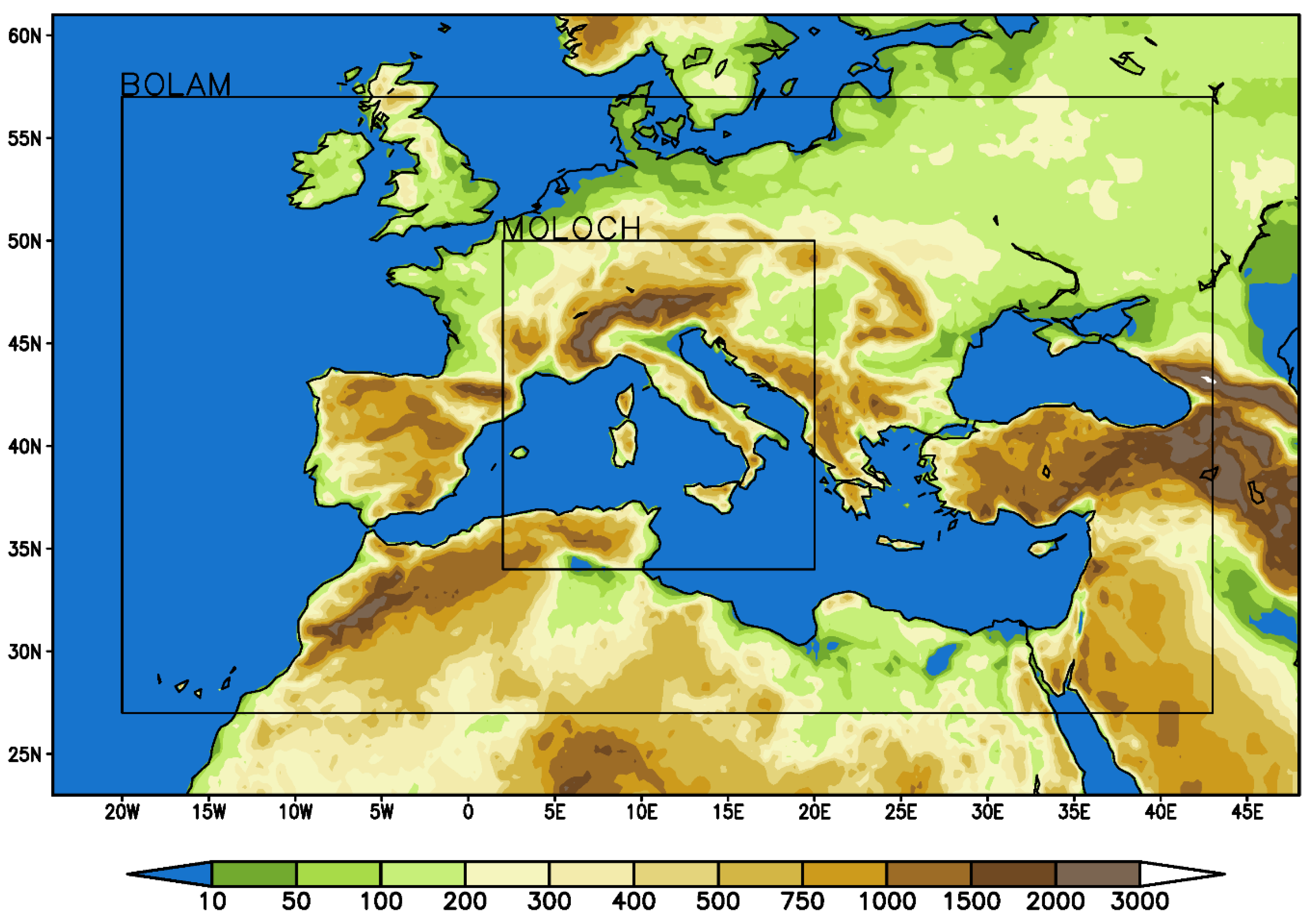
Figure 1.
Extent of the BOLAM and MOLOCH domains with superimposed topography. The BOLAM domain approximately corresponds to the Med-CORDEX domain [
53].
Figure 1.
Extent of the BOLAM and MOLOCH domains with superimposed topography. The BOLAM domain approximately corresponds to the Med-CORDEX domain [
53].
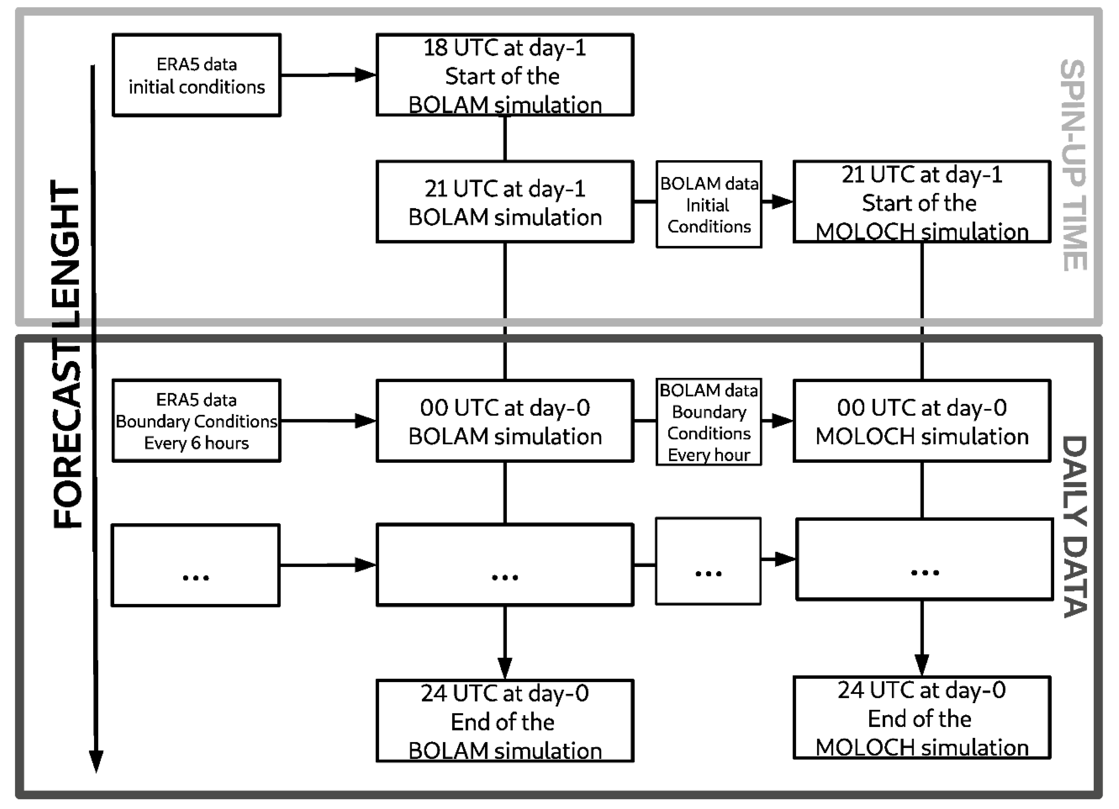
Figure 2.
Modelling setup for the production of one single day of data.
Figure 2.
Modelling setup for the production of one single day of data.
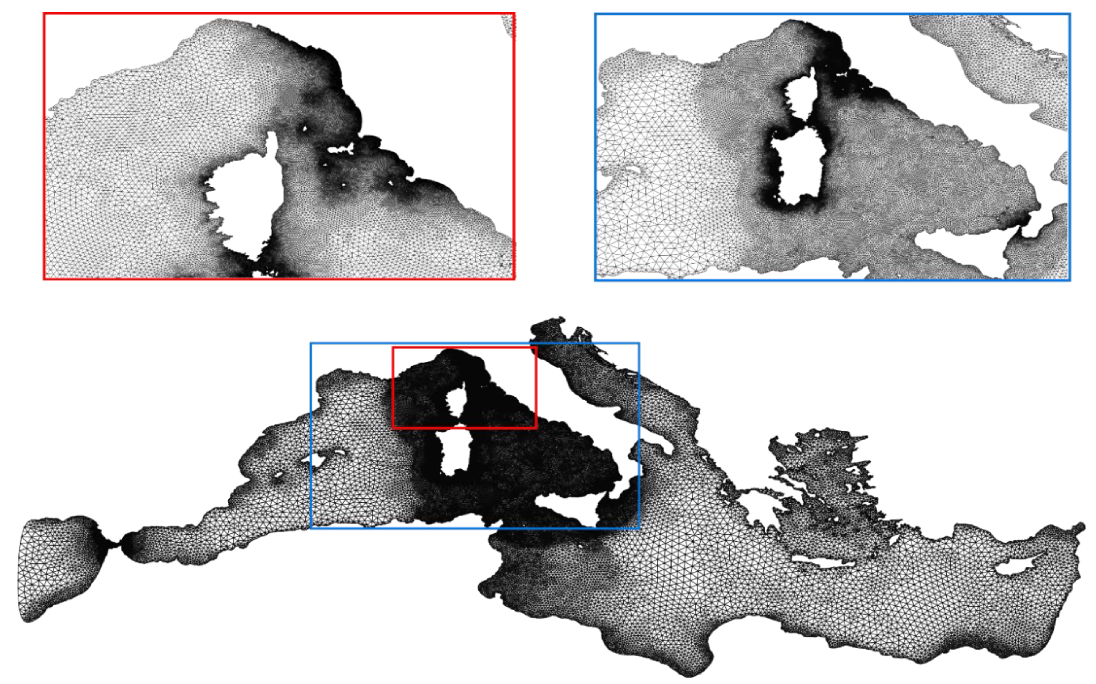
Figure 3.
Extent of the WaveWatch III (WW3) domain with enlarged views of North-Western Mediterranean Sea (light blue box) and Tuscany Archipelago and Eastern Ligurian Coast (red box).
Figure 3.
Extent of the WaveWatch III (WW3) domain with enlarged views of North-Western Mediterranean Sea (light blue box) and Tuscany Archipelago and Eastern Ligurian Coast (red box).
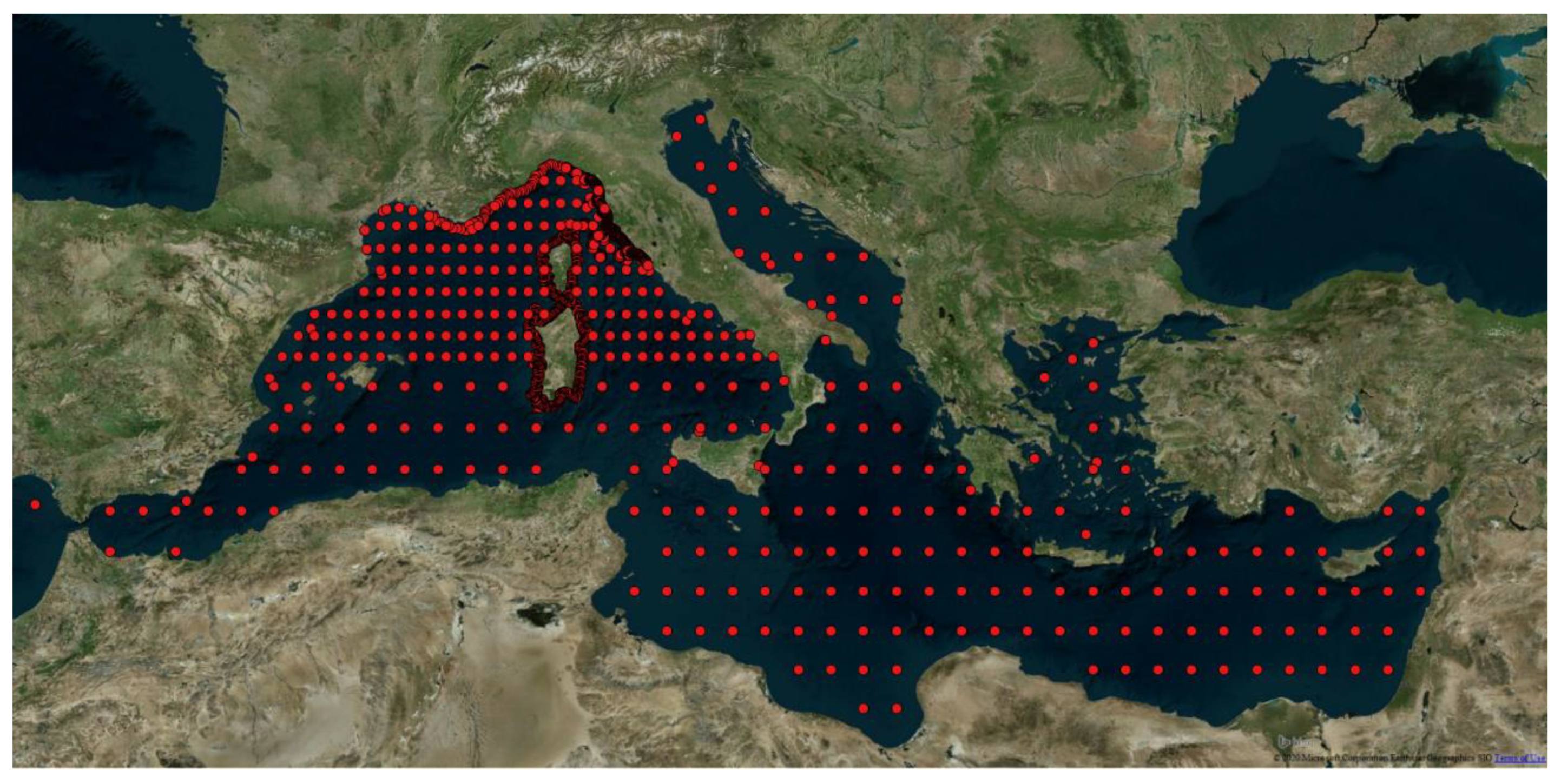
Figure 4.
Point output of the wave hindcast.
Figure 4.
Point output of the wave hindcast.
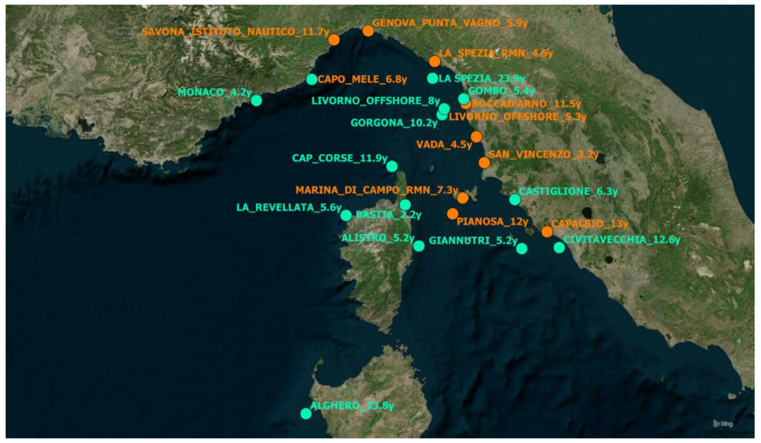
Figure 5.
Location of wind stations (orange points) and wave buoys (light green points) used to calibrate and validate the wind/wave hindcast. The length of the time series period is shown after the underscore (“_”) symbol following the name of the wind station or wave buoy.
Figure 5.
Location of wind stations (orange points) and wave buoys (light green points) used to calibrate and validate the wind/wave hindcast. The length of the time series period is shown after the underscore (“_”) symbol following the name of the wind station or wave buoy.
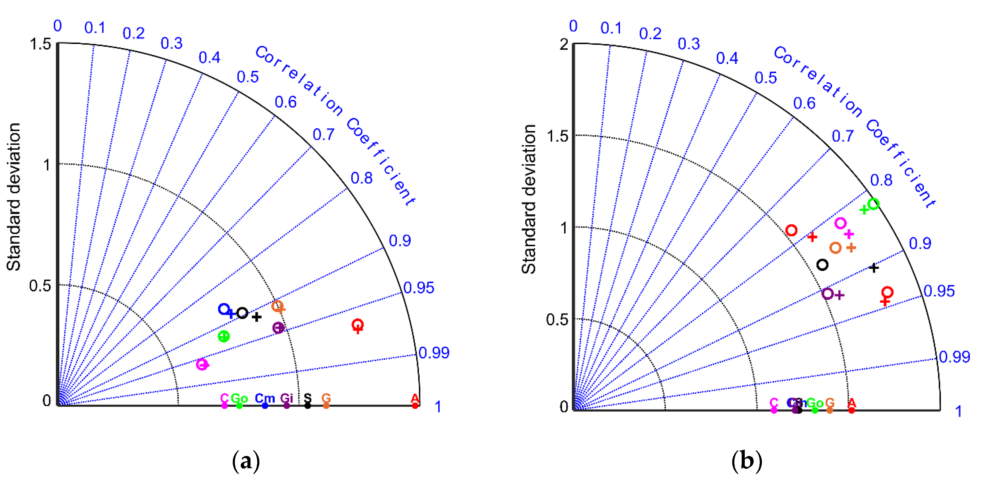
Figure 6.
Taylor diagram for the case studies in
Table 3. Results for Hs (
a) and Tm (
b) are reported. The plus symbols (+) and circle (◯) symbols refer to time steps equal to 60 and 120 s, respectively. Each buoy is represented by a different color: Alghero (A) in red, Capo Mele (Cm) in blue, Castiglione (C) in pink, Giannutri (Gi) in purple, Gombo (Go) in green, Gorgona (G) in orange and La Spezia (S) in black.
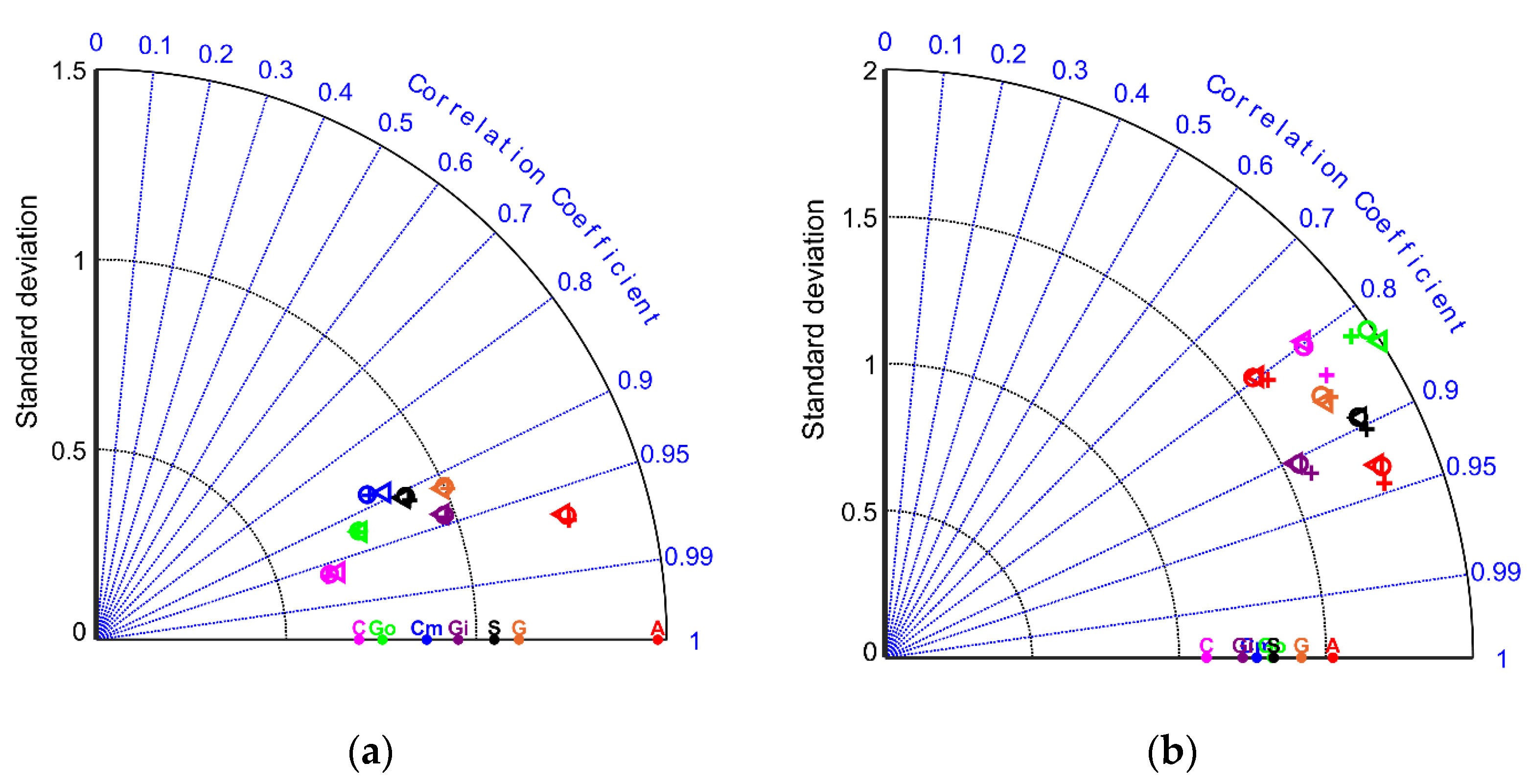
Figure 7.
Taylor diagrams for the case studies in
Table 3. Results are relative to Hs (
a) and Tm (
b) are reported. The plus (+), circle (◯) and triangle (⧍) symbols refer to the N scheme, PSI scheme and FCT scheme, respectively. Each buoy is represented by a different color: Alghero (A) in red, Capo Mele (Cm) in blue, Castiglione (C) in pink, Giannutri (Gi) in purple, Gombo (Go) in green, Gorgona (G) in orange and La Spezia (letter S) in black.
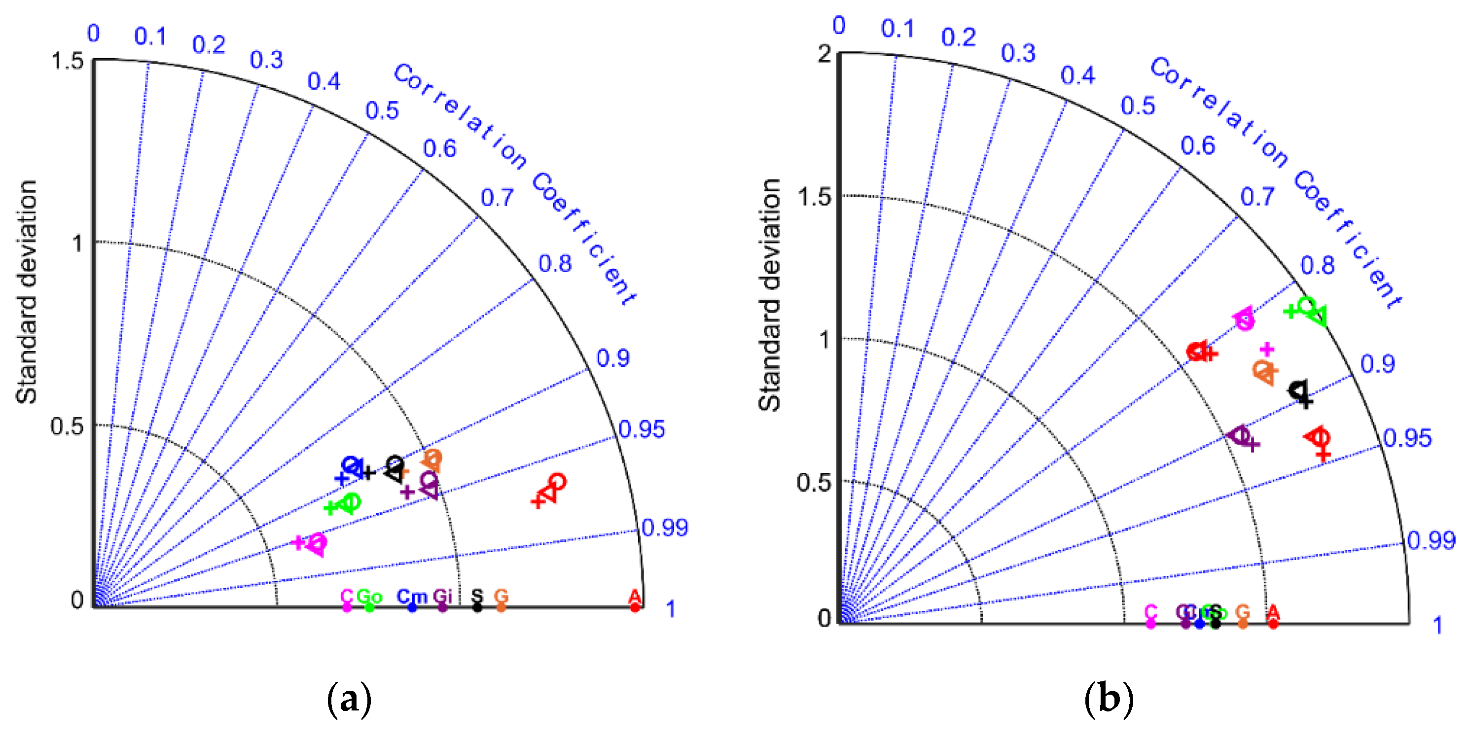
Figure 8.
Taylor diagrams for the case studies in
Table 3. Results for Hs (
a) and Tm (
b) are reported. The plus (+), circle (◯) and triangle (⧍) symbols refer to the ST2, ST3 and ST4 parametrizations, respectively. Each buoy is represented by a different color: Alghero (A) in red, Capo Mele (Cm) in blue, Castiglione (C) in pink, Giannutri (Gi) in purple, Gombo (Go) in green, Gorgona (G) in orange and La Spezia (letter S) in black.
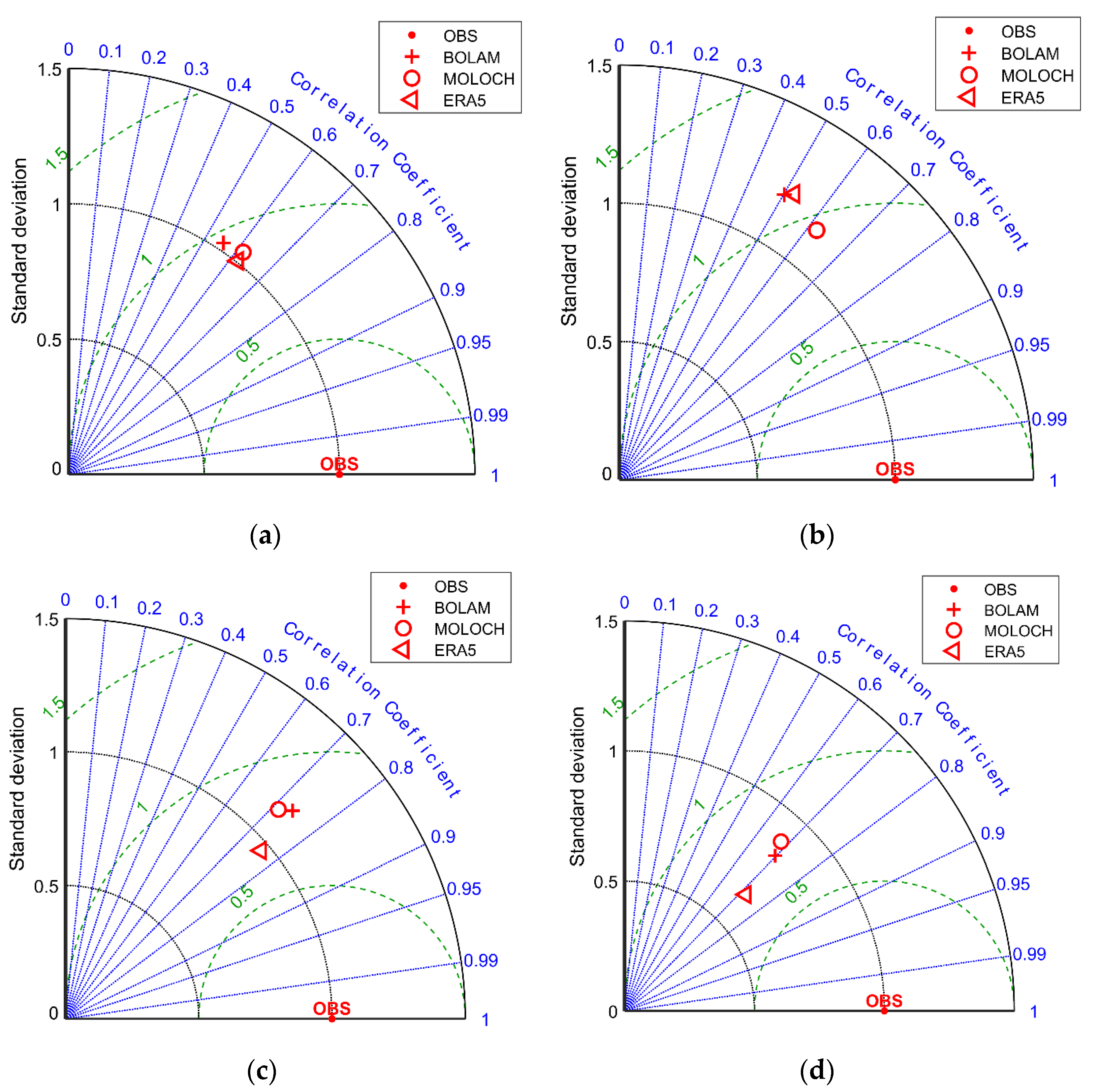
Figure 9.
Normalized Taylor diagrams for the: (a) Bocca d’Arno (no. 1), (b) Capalbio (no. 2), (c) Livorno offshore (no. 6) and (d) Vada (no. 11) wind stations. The plus (+), circle (◯) and triangle (⧍) symbols refer to the BOLAM, MOLOCH and ERA5 data, respectively.
Figure 9.
Normalized Taylor diagrams for the: (a) Bocca d’Arno (no. 1), (b) Capalbio (no. 2), (c) Livorno offshore (no. 6) and (d) Vada (no. 11) wind stations. The plus (+), circle (◯) and triangle (⧍) symbols refer to the BOLAM, MOLOCH and ERA5 data, respectively.
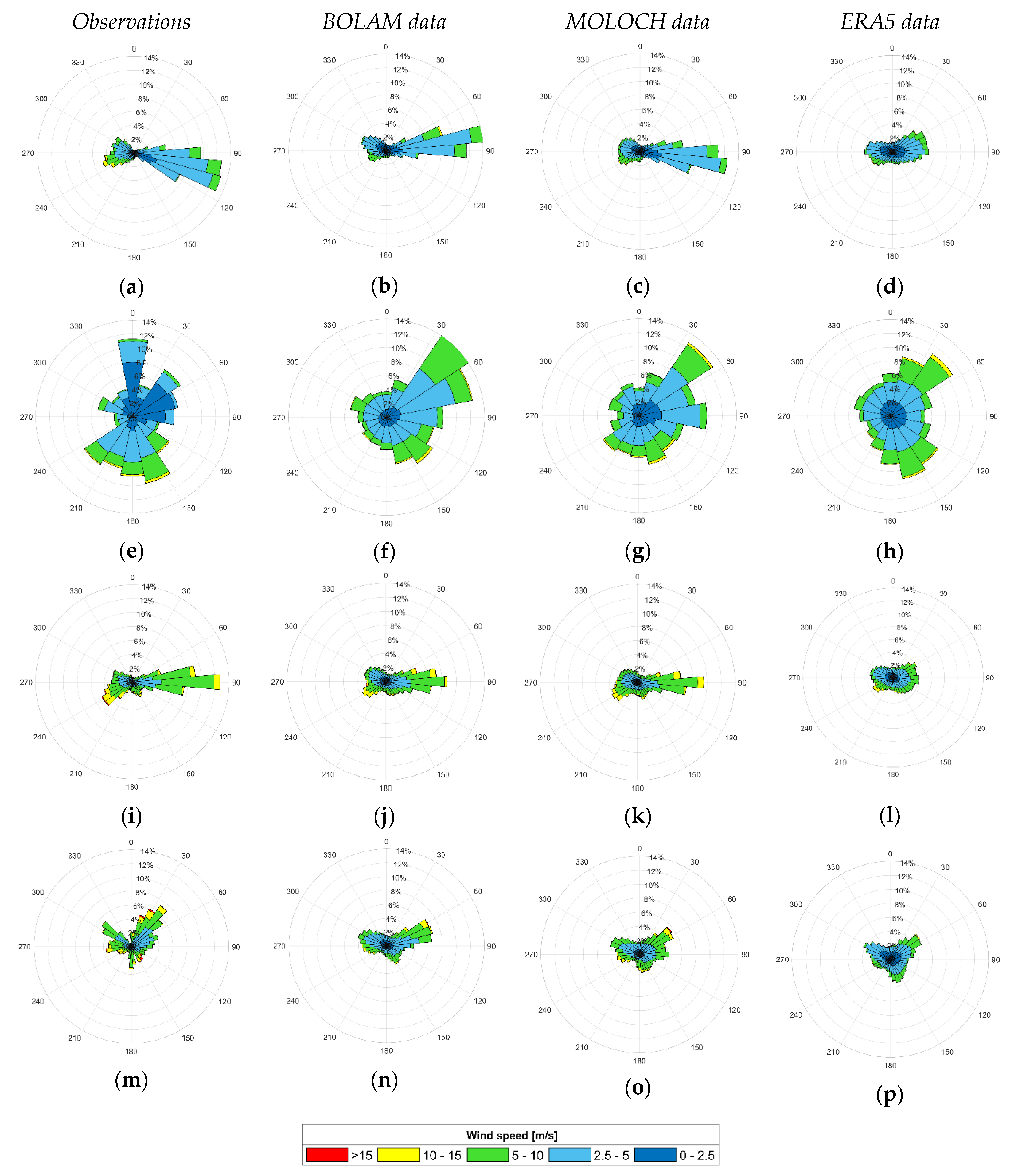
Figure 10.
Wind roses of velocity and direction for: (a) Bocca d’Arno (no. 1) wind station, (b) Bocca d’Arno BOLAM point, (c) Bocca d’Arno MOLOCH point, (d) Bocca d’Arno ERA5 point, (e) Capalbio (no. 2) wind station, (f) Capalbio BOLAM point, (g) Capalbio MOLOCH point, (h) Capalbio ERA5 point, (i) Livorno offshore (no. 6) wind station, (j) Livorno offshore BOLAM point, (k) Livorno offshore MOLOCH point, (l) Livorno offshore ERA5 point, (m) Vada (no. 11) wind station, (n) Vada BOLAM point, (o) Vada MOLOCH point, (p) Vada ERA5 point.
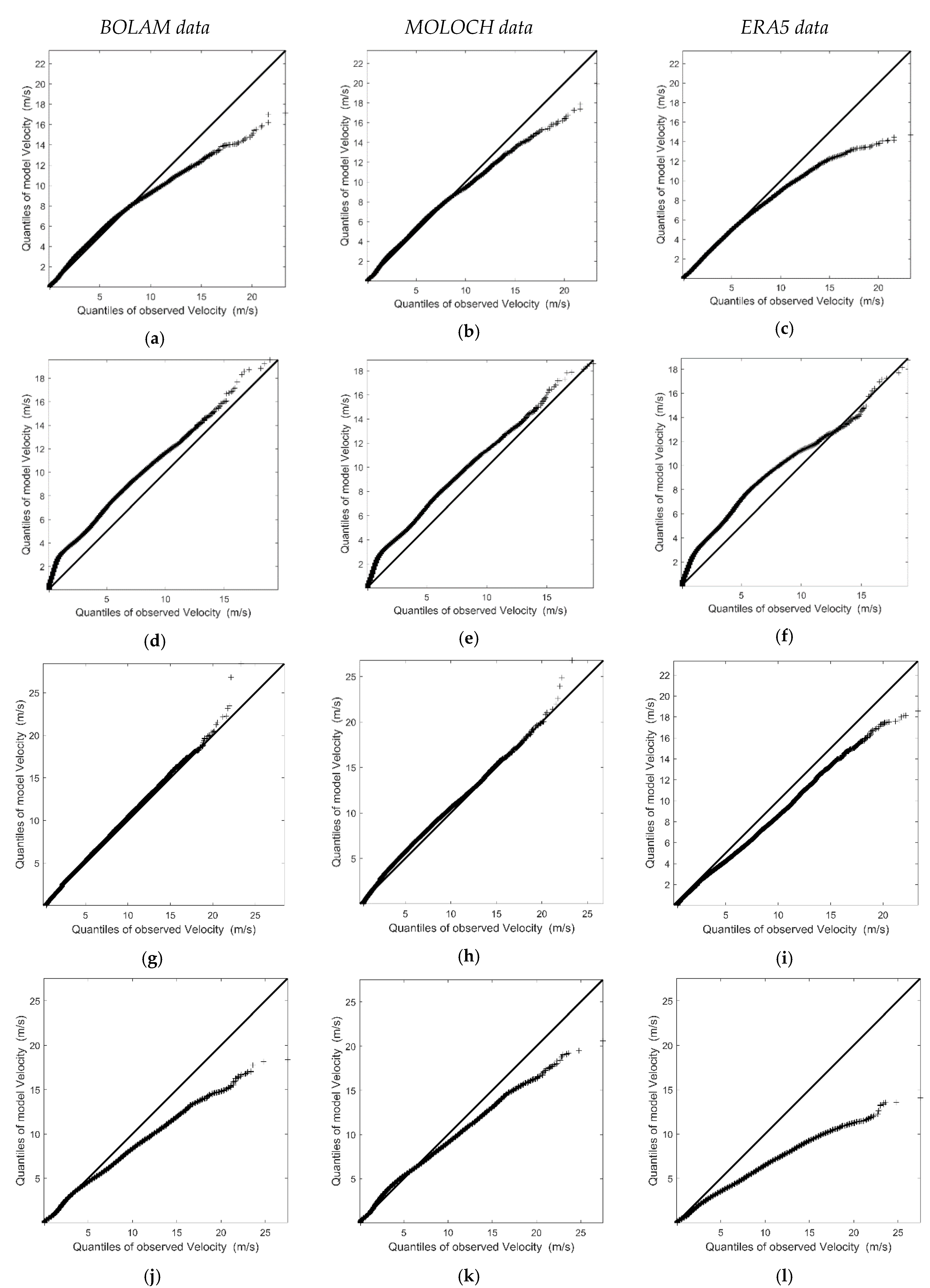
Figure 11.
Quantile-quantile (Q-Q) plots of the BOLAM (left), MOLOCH (center) or ERA5 (right) wind speed against the observed data at: (a–c) Bocca d’Arno (no. 1), (d–f) Capalbio (no. 2), (g–i) Livorno offshore (no. 6) (j–l) and Vada (no. 11) wind stations. Horizontal and vertical axes report observed and modelled data, respectively.
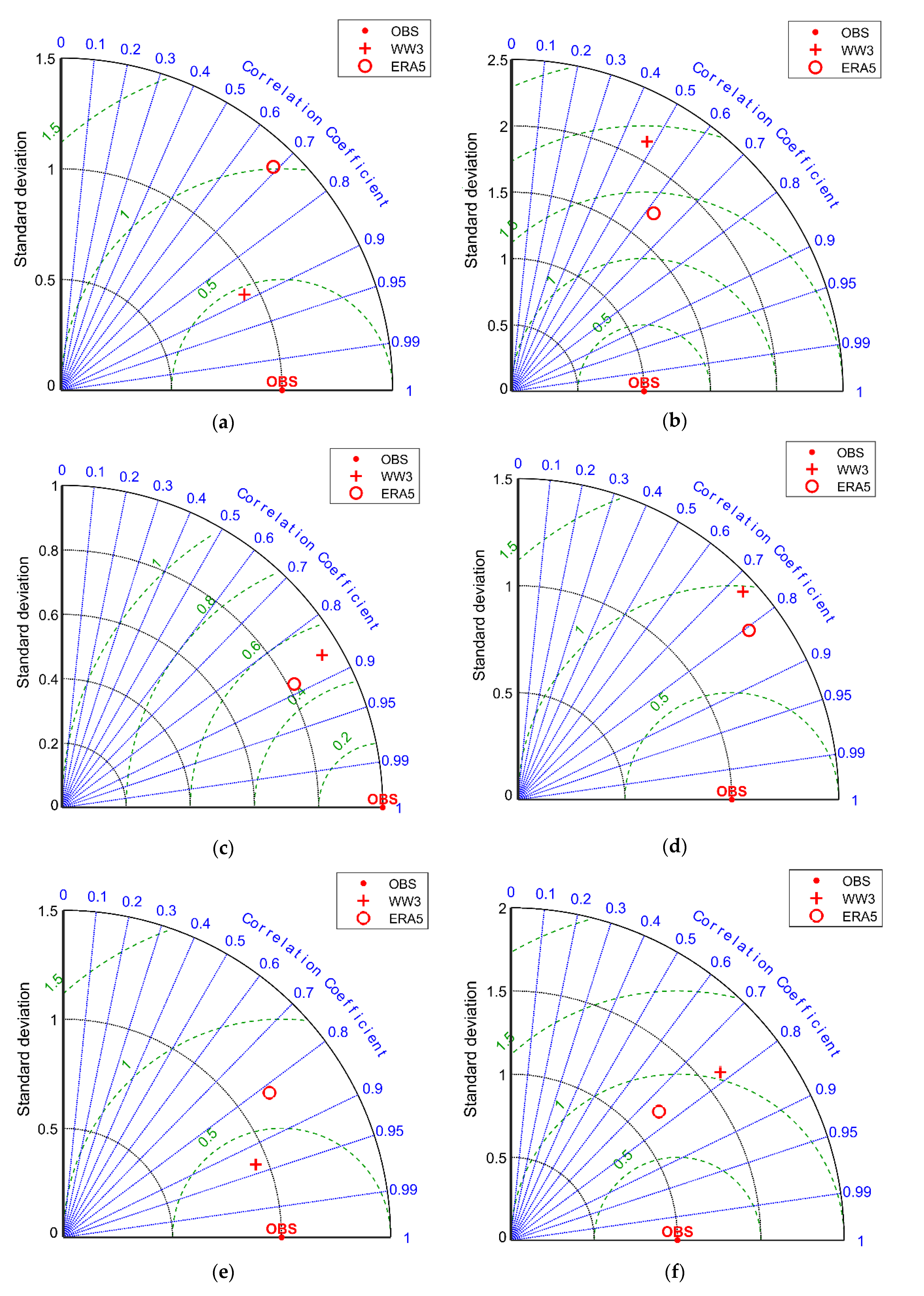
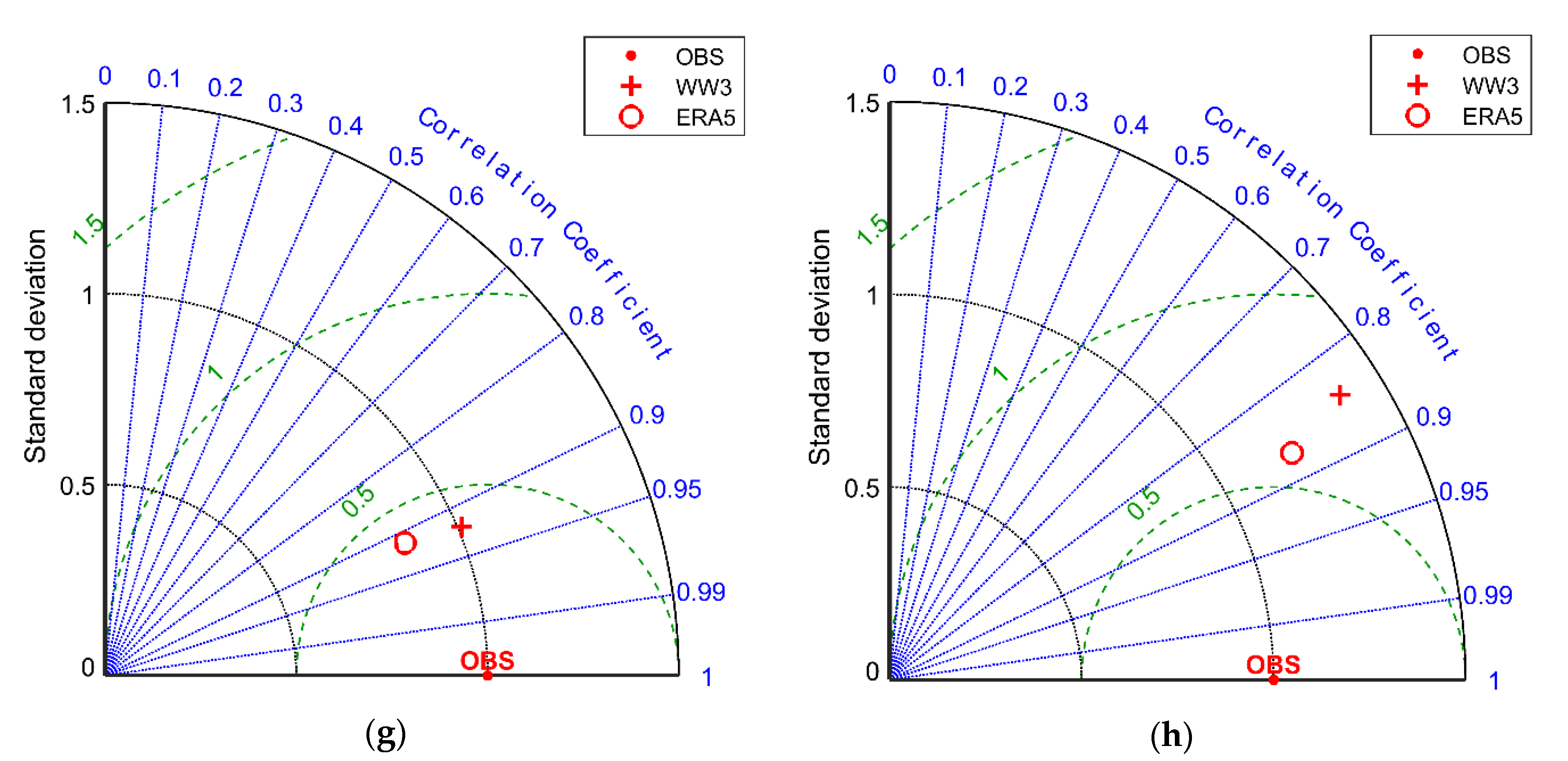
Figure 12.
Normalized Taylor diagrams for: (a,b) the Bastia (no. 3), (c,d) Capo Mele (no. 5), (e,f) Castiglione (no. 6), (g,h) Giannutri (no. 8) buoys. The results are relative to Hs (a,c,e,g) and Tm (b,d,f,h). The plus (+) and circle (◯) symbols refer to the wave hindcast (here WW3) and ERA5 data (here ERA5), respectively.
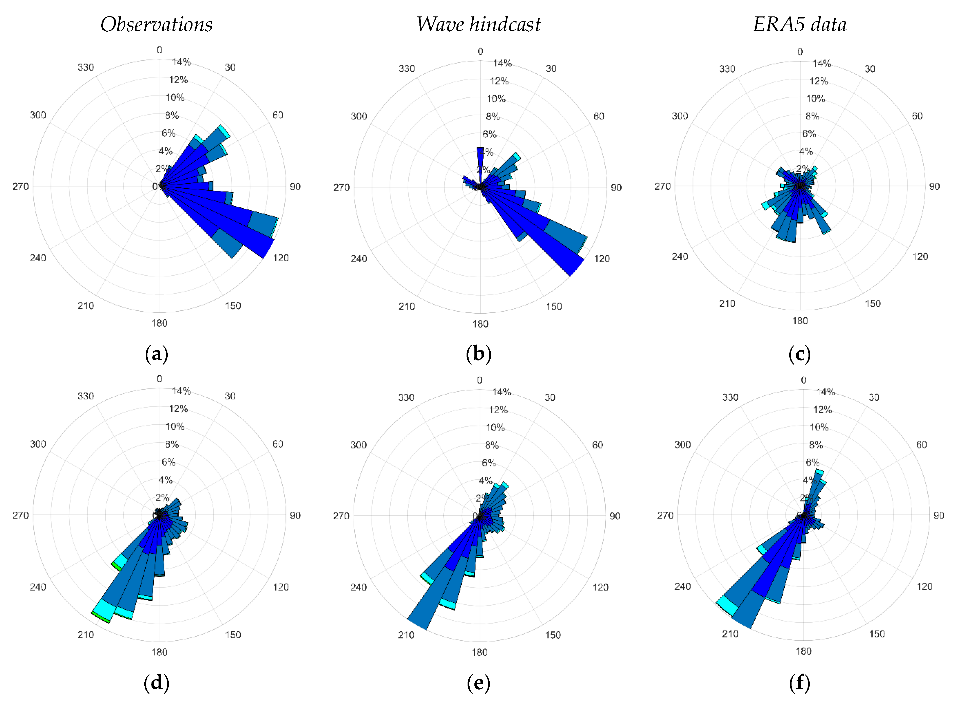
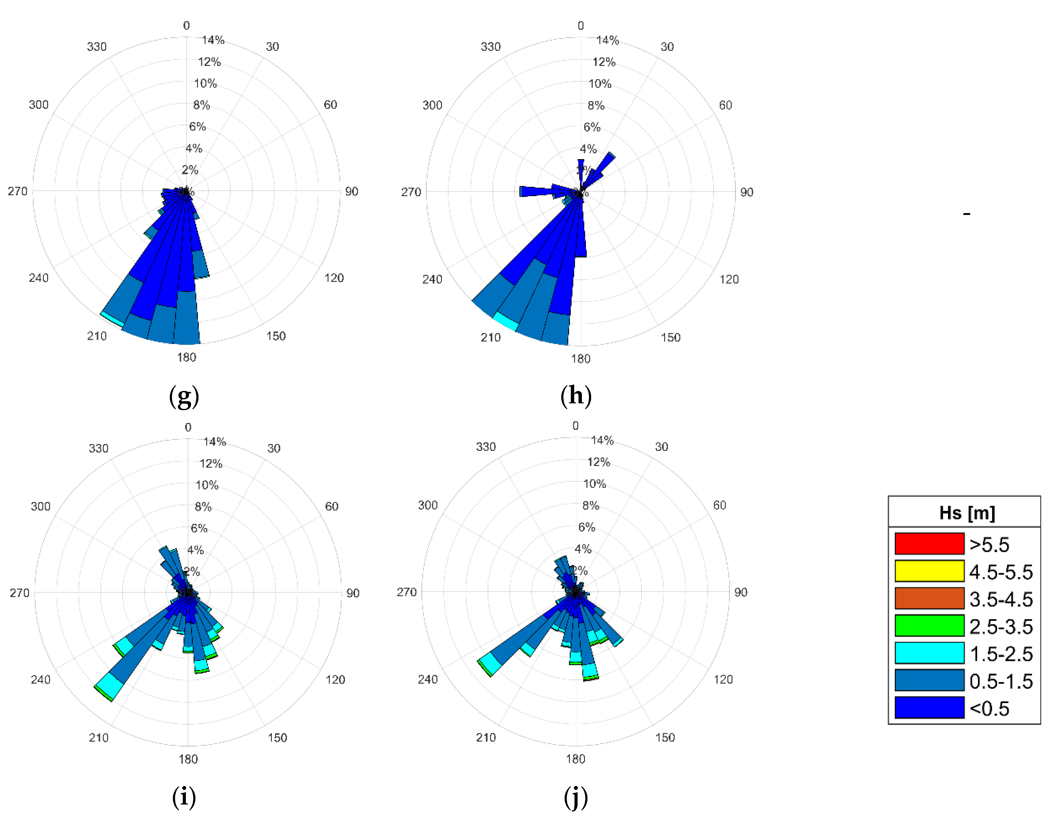
Figure 13.
Wave roses of Hs and Dirm for: (a) Bastia (no. 3) buoy; (b) Bastia wave hindcast point; (c) Bastia ERA5 point; (d) Capo Mele (no. 5) buoy; (e) Capo Mele wave hindcast point; (f) Capo Mele ERA5 point. Wave roses of Hs and Dirp for: (g) Castiglione (no. 6) buoy; (h) Castiglione wave hindcast point; (i) Giannutri (no. 8) buoy; (j) Giannutri wave hindcast point.
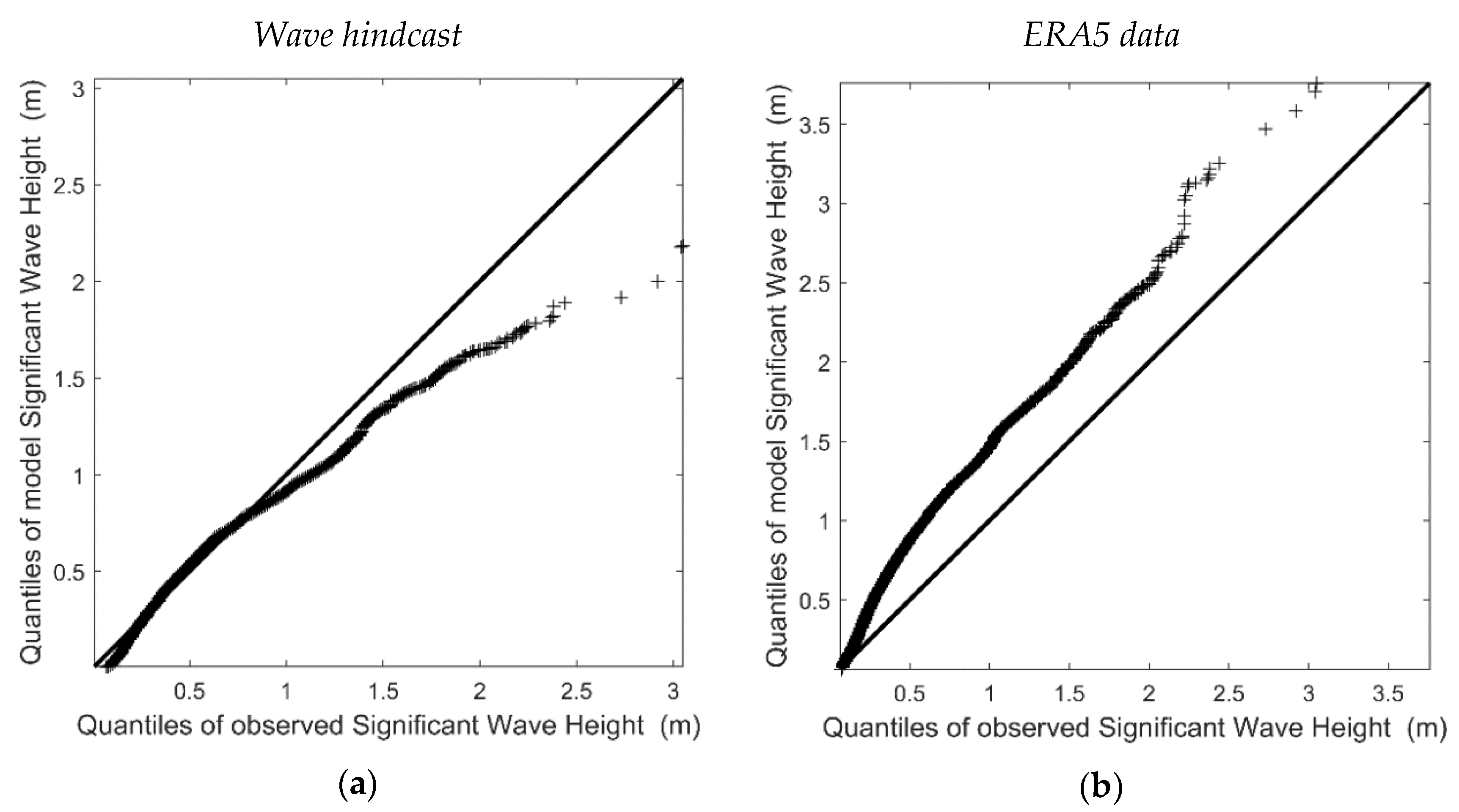
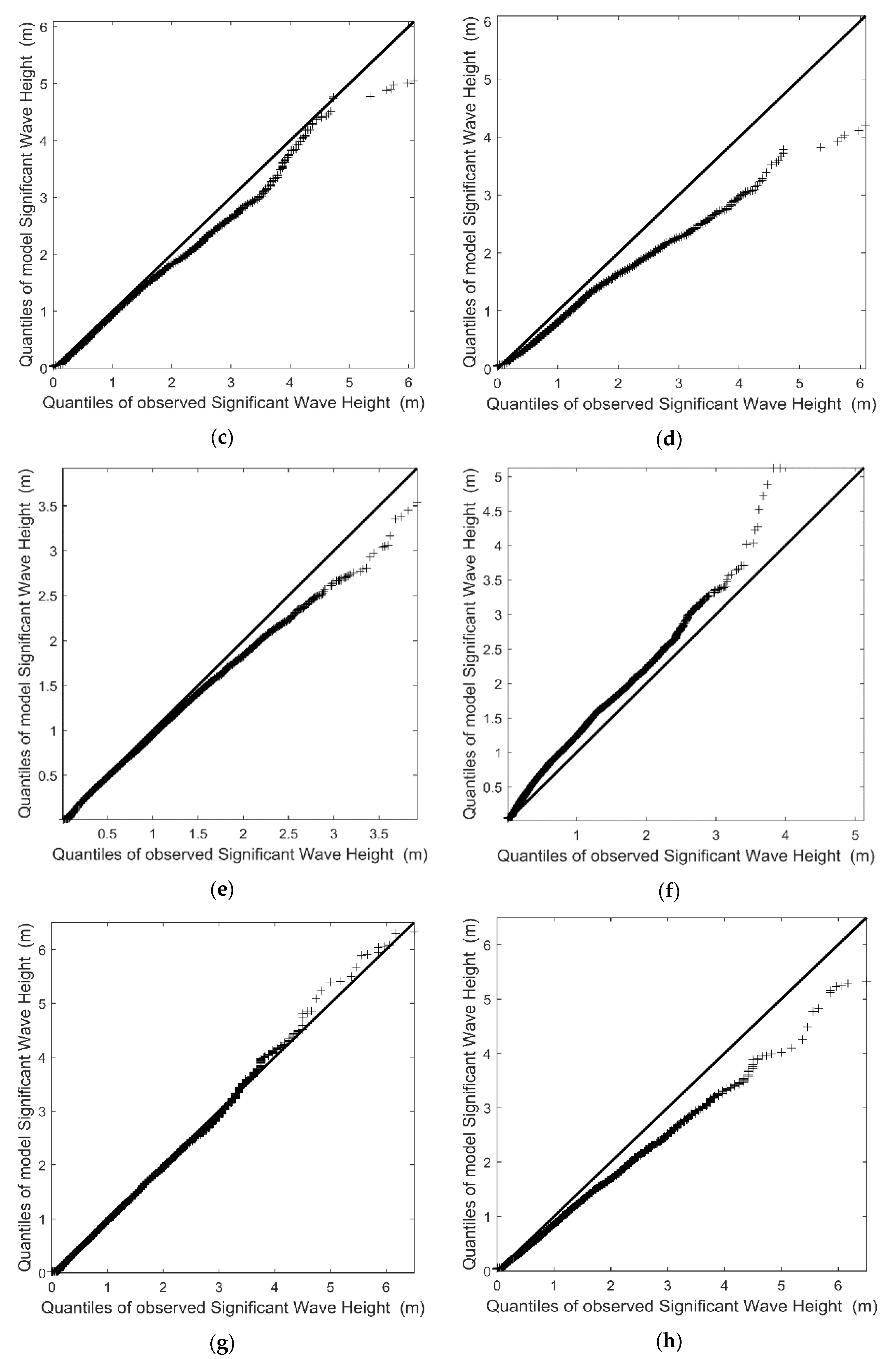
Figure 14.
Q-Q plots of significant wave heights of the wave hindcast (left column) or ERA5 dataset (right column) against the Bastia (no. 3), Capo Mele (no. 5), Castiglione (no. 6), Giannutri (no. 8) buoys. Horizontal and vertical axes report observed and modelled data, respectively.
Figure 14.
Q-Q plots of significant wave heights of the wave hindcast (left column) or ERA5 dataset (right column) against the Bastia (no. 3), Capo Mele (no. 5), Castiglione (no. 6), Giannutri (no. 8) buoys. Horizontal and vertical axes report observed and modelled data, respectively.
Table 1.
Setup of the key characteristics of the BOLAM and MOLOCH simulations.
Table 1.
Setup of the key characteristics of the BOLAM and MOLOCH simulations.
| | BOLAM | MOLOCH |
|---|
| Grid spacing (km) | 7 | 2.5 |
| Number of rows and columns | 482 and 890 | 626 and 506 |
| Number of vertical levels | 50 |
| Number of soil levels | 7 |
| Grid points | ~21.5 million | ~15.8 million |
| Time step (s) | 45 | 30 |
| Radiation scheme | Morcrette [49] and ECMWF radiation scheme [50] |
| Boundary layer scheme | 1.5-order E-l closure [51] |
| Microphysics scheme | Drofa and Malguzzi [48] |
| Turbulence scheme | 1.5-order E-l closure [52] |
| Convection parameterization | Kain [47] | none |
Table 2.
Wind stations with locations, time periods used to validate model data, and percentages of gaps in the mean wind velocity (V) records.
Table 2.
Wind stations with locations, time periods used to validate model data, and percentages of gaps in the mean wind velocity (V) records.
| No. | Station | Lon (°) | Lat (°) | Start Date | End Date | Missing Data (%) | P33 (m/s) |
|---|
| 1 | BOCCA D’ARNO | 10.28 | 43.68 | 13/06/2007 | 31/12/2018 | 2.1 | 2.0 |
| 2 | CAPALBIO | 11.39 | 42.41 | 06/12/2005 | 31/12/2018 | 18.4 | 1.1 |
| 3 | CAPO MELE | 8.18 | 43.92 | 23/02/2012 | 31/12/2018 | 0.2 | 2.7 |
| 4 | GENOVA-PUNTA_VAGNO | 8.95 | 44.39 | 17/01/2013 | 31/12/2018 | 1.3 | 2.5 |
| 5 | LA SPEZIA RMN | 9.86 | 44.10 | 01/07/2010 | 23/01/2015 | 5.5 | 1.6 |
| 6 | LIVORNO OFFSHORE | 9.99 | 43.63 | 01/09/2013 | 31/12/2018 | 1.8 | 2.8 |
| 7 | MARINA DI CAMPO RMN | 10.24 | 42.74 | 21/07/2011 | 12/12/2018 | 6.9 | 1.7 |
| 8 | PIANOSA | 10.10 | 42.59 | 01/01/2000 | 01/01/2012 | 31.1 | 1.5 |
| 9 | SAN VINCENZO | 10.54 | 43.10 | 04/10/2015 | 31/12/2018 | 1.7 | 1.6 |
| 10 | SAVONA ISTITUTO NAUTICO | 8.48 | 44.31 | 18/04/2007 | 31/12/2018 | 1.3 | 2.2 |
| 11 | VADA | 10.43 | 43.36 | 15/04/2010 | 20/10/2014 | 29.4 | 2.8 |
Table 3.
Buoy stations with locations, water depths, time periods used to validate model data and percentages of gaps in the significant wave height (Hs) records. The wave direction was not available for buoy number 4.
Table 3.
Buoy stations with locations, water depths, time periods used to validate model data and percentages of gaps in the significant wave height (Hs) records. The wave direction was not available for buoy number 4.
| No. | Station | Lon (°) | Lat (°) | Water Depth (m) | Start Date | End Date | Missing Data (%) |
|---|
| 1a | ALGHERO1 | 8.11 | 40.55 | 85 1 | 01/07/1989 | 01/01/2001 | 3.6 2 |
| 1b | ALGHERO2 | 8.11 | 40.55 | 85 1 | 15/06/2002 | 30/10/2014 | 41.3 |
| 2 | ALISTRO | 9.64 | 42.26 | 120 3 | 15/10/2013 | 31/12/2018 | 34.7 |
| 3 | BASTIA | 9.45 | 42.67 | 17 3 | 13/09/2006 | 19/11/2008 | 39.0 |
| 4 | CAP CORSE | 9.28 | 43.06 | 140 3 | 16/03/1999 | 01/03/2011 | 53.6 2 |
| 5 | CAPO MELE | 8.18 | 43.92 | 80 4 | 01/03/2012 | 31/12/2018 | 24.8 |
| 6 | CASTIGLIONE | 10.95 | 42.73 | 15 4 | 23/09/2012 | 31/12/2018 | 23.2 |
| 7 | CIVITAVECCHIA | 11.55 | 42.24 | 62 4 | 30/04/2002 | 23/12/2014 | 50.9 |
| 8 | GIANNUTRI | 11.05 | 42.24 | 140 4 | 01/10/2013 | 31/12/2018 | 8 |
| 9 | GOMBO | 10.25 | 43.73 | 15 4 | 17/07/2013 | 31/12/2018 | 52.8 |
| 10 | GORGONA | 9.96 | 43.57 | 140 4 | 01/10/2008 | 31/12/2018 | 3.6 |
| 11 | LA REVELLATA | 8.65 | 42.57 | 130 3 | 02/05/2013 | 31/12/2018 | 26 |
| 12a | LA SPEZIA1 | 9.83 | 43.93 | 85 1 | 01/07/1989 | 01/01/2001 | 7.32 2 |
| 12b | LA SPEZIA2 | 9.83 | 43.93 | 85 1 | 12/07/2002 | 29/12/2014 | 41.5 |
| 13 | LIVORNO OFFSHORE | 9.99 | 43.63 | 115 4 | 21/12/2010 | 31/12/2018 | 20.8 |
| 14 | MONACO | 7.43 | 43.71 | 924 3 | 29/10/2014 | 31/12/2018 | 10.4 |
Table 4.
Time period of the case studies considered for calibration analysis. In the last two columns we also report the observed maximum significant wave height and corresponding mean period.
Table 4.
Time period of the case studies considered for calibration analysis. In the last two columns we also report the observed maximum significant wave height and corresponding mean period.
| No. | Case Study | Start Date | End Date | Max Hs (m) | Tm (s) |
|---|
| 1 | March 2010 | 24/03/2010 | 06/04/2010 | 4.70 | 7.55 |
| 2 | December 2011 | 06/12/2011 | 21/12/2011 | 7.28 | 9.29 |
| 3 | March 2013 | 09/03/2013 | 20/03/2013 | 6.82 | 8.63 |
| 4 | May 2013 | 15/05/2013 | 30/05/2013 | 5.03 | 7.90 |
| 5 | December 2013 | 16/12/2013 | 30/12/2013 | 7.94 | 9.70 |
| 6 | October 2014 | 26/10/2014 | 07/11/2014 | 4.73 | 8.20 |
| 7 | January 2015 | 21/01/2015 | 03/02/2015 | 5.20 | 8.24 |
| 8 | January 2016 | 01/01/2016 | 18/01/2016 | 6.61 | 8.44 |
| 9 | October 2016 | 05/10/2016 | 18/10/2016 | 4.34 | 7.20 |
| 10 | December 2016 | 11/12/2016 | 24/12/2016 | 4.11 | 7.99 |
| 11 | December 2017 | 02/12/2017 | 20/12/2017 | 5.18 | 8.04 |
| 12 | October 2018 | 19/10/2018 | 02/11/2018 | 6.50 | 8.89 |
Table 5.
Statistical indicators for Hs, mean wave period (Tm) and peak wave direction (Dirp) (or mean wave direction (Dirm)), evaluated for time steps equal to 120 and 60 s with ST4 source term parameterization and explicit N scheme.
Table 5.
Statistical indicators for Hs, mean wave period (Tm) and peak wave direction (Dirp) (or mean wave direction (Dirm)), evaluated for time steps equal to 120 and 60 s with ST4 source term parameterization and explicit N scheme.
| Buoy | Time Step (s) | Hs (m) | Tm (s) | Dirp (°N) |
|---|
| No. 1 | MBE | MAE | RMSE | cRMSE | r | MBE | MAE | RMSE | cRMSE | r | circ-r |
|---|
| 1 | 60 | −0.15 | 0.29 | 0.42 | 0.39 | 0.97 | 0.9 | 0.97 | 1.09 | 0.62 | 0.94 | 0.88 |
| 120 | −0.16 | 0.31 | 0.44 | 0.41 | 0.97 | 0.87 | 0.97 | 1.1 | 0.67 | 0.94 | 0.87 |
| 5 | 60 | −0.07 | 0.3 | 0.43 | 0.43 | 0.87 | −0.14 | 0.77 | 0.98 | 0.97 | 0.79 | 0.451 2 |
| | 120 | −0.07 | 0.3 | 0.44 | 0.43 | 0.87 | −0.11 | 0.77 | 0.99 | 0.98 | 0.77 | 0.451 2 |
| 6 | 60 | −0.06 | 0.13 | 0.19 | 0.19 | 0.96 | 0.83 | 1.05 | 1.33 | 1.04 | 0.84 | 0.41 |
| | 120 | −0.06 | 0.14 | 0.2 | 0.19 | 0.96 | 0.75 | 1.05 | 1.32 | 1.08 | 0.82 | 0.44 |
| 8 | 60 | −0.03 | 0.22 | 0.32 | 0.32 | 0.94 | 0.36 | 0.57 | 0.76 | 0.67 | 0.92 | 0.64 |
| | 120 | −0.03 | 0.23 | 0.32 | 0.32 | 0.94 | 0.38 | 0.58 | 0.76 | 0.66 | 0.91 | 0.62 |
| 9 | 60 | −0.03 | 0.19 | 0.29 | 0.29 | 0.93 | 0.75 | 1.04 | 1.35 | 1.13 | 0.82 | 0.42 |
| | 120 | −0.03 | 0.2 | 0.3 | 0.29 | 0.92 | 0.7 | 1.05 | 1.37 | 1.17 | 0.82 | 0.4 |
| 10 | 60 | −0.17 | 0.32 | 0.47 | 0.44 | 0.92 | 0.36 | 0.74 | 0.96 | 0.89 | 0.86 | 0.67 |
| 120 | −0.17 | 0.33 | 0.49 | 0.46 | 0.91 | 0.39 | 0.75 | 0.97 | 0.89 | 0.85 | 0.69 |
| 12 | 60 | −0.21 | 0.34 | 0.48 | 0.43 | 0.91 | 0.82 | 0.97 | 1.17 | 0.84 | 0.9 | 0.69 |
| 120 | −0.23 | 0.37 | 0.52 | 0.47 | 0.89 | 0.89 | 1.01 | 1.2 | 0.8 | 0.86 | 0.76 |
Table 6.
Statistical indicators for Hs, Tm and Dirp (or Dirm), evaluated for explicit N, PSI and FCT numerical schemes, with ST4 source term parameterization and 60 s time step.
Table 6.
Statistical indicators for Hs, Tm and Dirp (or Dirm), evaluated for explicit N, PSI and FCT numerical schemes, with ST4 source term parameterization and 60 s time step.
| Buoy No. 1 | Numerical Scheme | Hs (m) | Tm (s) | Dirp (°N) |
|---|
| MBE | MAE | RMSE | cRMSE | r | MBE | MAE | RMSE | cRMSE | r | circ-r |
|---|
| 1 | N | −0.15 | 0.29 | 0.42 | 0.39 | 0.97 | 0.90 | 0.97 | 1.09 | 0.62 | 0.94 | 0.88 |
| PSI | −0.15 | 0.3 | 0.43 | 0.41 | 0.97 | 0.88 | 0.98 | 1.11 | 0.67 | 0.93 | 0.86 |
| FCT | −0.17 | 0.31 | 0.45 | 0.41 | 0.97 | 0.86 | 0.97 | 1.09 | 0.67 | 0.93 | 0.85 |
| 5 | N | −0.07 | 0.3 | 0.43 | 0.43 | 0.87 | −0.14 | 0.77 | 0.98 | 0.97 | 0.79 | 0.451 2 |
| PSI | −0.07 | 0.3 | 0.44 | 0.43 | 0.87 | −0.12 | 0.77 | 0.99 | 0.98 | 0.77 | 0.441 2 |
| FCT | −0.02 | 0.29 | 0.42 | 0.42 | 0.88 | −0.05 | 0.77 | 0.99 | 0.98 | 0.77 | 0.421 2 |
| 6 | N | −0.06 | 0.13 | 0.19 | 0.19 | 0.96 | 0.83 | 1.05 | 1.33 | 1.04 | 0.84 | 0.41 |
| PSI | −0.05 | 0.13 | 0.19 | 0.19 | 0.96 | 0.84 | 1.11 | 1.39 | 1.11 | 0.80 | 0.40 |
| FCT | −0.03 | 0.13 | 0.19 | 0.19 | 0.96 | 0.88 | 1.14 | 1.43 | 1.13 | 0.80 | 0.39 |
| 8 | N | −0.03 | 0.22 | 0.32 | 0.32 | 0.94 | 0.36 | 0.57 | 0.76 | 0.67 | 0.92 | 0.64 |
| PSI | −0.02 | 0.23 | 0.33 | 0.33 | 0.94 | 0.38 | 0.59 | 0.78 | 0.69 | 0.91 | 0.63 |
| FCT | −0.02 | 0.23 | 0.33 | 0.33 | 0.94 | 0.38 | 0.59 | 0.78 | 0.69 | 0.90 | 0.61 |
| 9 | N | −0.03 | 0.19 | 0.29 | 0.29 | 0.93 | 0.75 | 1.04 | 1.35 | 1.13 | 0.82 | 0.42 |
| PSI | −0.03 | 0.2 | 0.29 | 0.29 | 0.92 | 0.69 | 1.04 | 1.35 | 1.16 | 0.83 | 0.40 |
| FCT | −0.02 | 0.19 | 0.29 | 0.29 | 0.93 | 0.74 | 1.04 | 1.35 | 1.14 | 0.84 | 0.42 |
| 10 | N | −0.17 | 0.32 | 0.47 | 0.44 | 0.92 | 0.36 | 0.74 | 0.96 | 0.89 | 0.86 | 0.67 |
| PSI | −0.18 | 0.33 | 0.48 | 0.45 | 0.92 | 0.32 | 0.73 | 0.95 | 0.89 | 0.86 | 0.67 |
| FCT | −0.18 | 0.33 | 0.48 | 0.45 | 0.92 | 0.3 | 0.71 | 0.93 | 0.87 | 0.87 | 0.67 |
| 12 | N | −0.21 | 0.34 | 0.48 | 0.43 | 0.91 | 0.82 | 0.97 | 1.17 | 0.84 | 0.90 | 0.69 |
| PSI | −0.23 | 0.35 | 0.5 | 0.44 | 0.91 | 0.75 | 0.94 | 1.15 | 0.87 | 0.89 | 0.68 |
| FCT | −0.23 | 0.35 | 0.5 | 0.44 | 0.91 | 0.78 | 0.96 | 1.17 | 0.87 | 0.89 | 0.65 |
Table 7.
Statistical indicators for Hs, Tm and Dirp (or Dirm) evaluated for the ST2, ST3 and ST4 source term parameterizations with 60 s time step and N scheme.
Table 7.
Statistical indicators for Hs, Tm and Dirp (or Dirm) evaluated for the ST2, ST3 and ST4 source term parameterizations with 60 s time step and N scheme.
| Buoy No. 1 | Source Term Param. | Hs (m) | Tm (s) | Dirp (°N) |
|---|
| MBE | MAE | RMSE | cRMSE | r | MBE | MAE | RMSE | cRMSE | r | circ-r |
|---|
| 1 | ST2 | −0.20 | 0.29 | 0.44 | 0.39 | 0.97 | 0.46 | 0.66 | 0.79 | 0.64 | 0.93 | 0.86 |
| ST3 | −0.19 | 0.31 | 0.45 | 0.40 | 0.96 | 1.02 | 1.15 | 1.31 | 0.81 | 0.93 | 0.87 |
| ST4 | −0.15 | 0.29 | 0.42 | 0.39 | 0.97 | 0.90 | 0.97 | 1.09 | 0.62 | 0.94 | 0.88 |
| 5 | ST2 | −0.20 | 0.33 | 0.46 | 0.42 | 0.87 | −0.52 | 0.87 | 1.17 | 1.05 | 0.73 | 0.441 2 |
| ST3 | −0.12 | 0.32 | 0.46 | 0.44 | 0.86 | −0.11 | 0.88 | 1.11 | 1.1 | 0.74 | 0.451 2 |
| ST4 | −0.07 | 0.30 | 0.43 | 0.43 | 0.87 | −0.14 | 0.77 | 0.98 | 0.97 | 0.79 | 0.451 2 |
| 6 | ST2 | −0.12 | 0.17 | 0.25 | 0.22 | 0.95 | 0.35 | 0.88 | 1.18 | 1.12 | 0.83 | 0.49 |
| ST3 | −0.07 | 0.14 | 0.21 | 0.2 | 0.96 | 0.76 | 1.11 | 1.45 | 1.24 | 0.84 | 0.45 |
| ST4 | −0.06 | 0.13 | 0.19 | 0.19 | 0.96 | 0.83 | 1.05 | 1.33 | 1.04 | 0.84 | 0.41 |
| 8 | ST2 | −0.12 | 0.25 | 0.35 | 0.33 | 0.94 | −0.03 | 0.53 | 0.67 | 0.67 | 0.90 | 0.60 |
| ST3 | −0.05 | 0.25 | 0.35 | 0.35 | 0.93 | 0.44 | 0.68 | 0.89 | 0.77 | 0.90 | 0.58 |
| ST4 | −0.03 | 0.22 | 0.32 | 0.32 | 0.94 | 0.36 | 0.57 | 0.76 | 0.67 | 0.92 | 0.64 |
| 9 | ST2 | −0.10 | 0.21 | 0.31 | 0.29 | 0.92 | 0.15 | 0.98 | 1.23 | 1.22 | 0.80 | 0.32 |
| ST3 | −0.04 | 0.2 | 0.3 | 0.29 | 0.92 | 0.52 | 1.11 | 1.44 | 1.35 | 0.80 | 0.32 |
| ST4 | −0.03 | 0.19 | 0.29 | 0.29 | 0.93 | 0.75 | 1.04 | 1.35 | 1.13 | 0.82 | 0.42 |
| 10 | ST2 | −0.27 | 0.37 | 0.53 | 0.46 | 0.91 | −0.11 | 0.68 | 0.90 | 0.90 | 0.84 | 0.63 |
| ST3 | −0.18 | 0.33 | 0.49 | 0.45 | 0.91 | 0.39 | 0.84 | 1.07 | 0.99 | 0.85 | 0.64 |
| ST4 | −0.17 | 0.32 | 0.47 | 0.44 | 0.92 | 0.36 | 0.74 | 0.96 | 0.89 | 0.86 | 0.67 |
| | ST2 | −0.31 | 0.39 | 0.57 | 0.47 | 0.90 | 0.3 | 0.66 | 0.84 | 0.79 | 0.88 | 0.69 |
| 12 | ST3 | −0.25 | 0.36 | 0.51 | 0.45 | 0.90 | 0.83 | 1.05 | 1.28 | 0.97 | 0.88 | 0.69 |
| | ST4 | −0.21 | 0.34 | 0.48 | 0.43 | 0.91 | 0.82 | 0.97 | 1.17 | 0.84 | 0.90 | 0.69 |
Table 8.
Settings evaluated and kept constant in the calibration process and final selection.
Table 8.
Settings evaluated and kept constant in the calibration process and final selection.
| Calibration Setting | Selected | Evaluated | Constant |
|---|
| Maximum CFL time step for x-y and k-theta | 60 s | 60–120 s | N scheme, ST4 |
| Explicit numerical scheme | N | N-PSI-FCT | 60 s, ST4 |
| Source term parameterization | ST4 | ST2-ST3-ST4 | 60 s, N scheme |
Table 9.
Statistical indicators for wind speed and direction obtained for the wind speed values above the thresholds of the 33rd percentile.
Table 9.
Statistical indicators for wind speed and direction obtained for the wind speed values above the thresholds of the 33rd percentile.
| Wind Station | Atmospheric | Wind Speed (m/s) | Dir (°N) |
|---|
| No. 1 | Model | MBE | MAE | RMSE | cRMSE | r | circ-r |
|---|
| 1 | BOLAM | −0.09 | 1.41 | 1.90 | 1.90 | 0.56 | 0.19 |
| MOLOCH | −0.11 | 1.29 | 1.78 | 1.78 | 0.62 | 0.67 |
| ERA5 | −0.47 | 1.35 | 1.80 | 1.74 | 0.62 | 0.64 |
| 2 | BOLAM | 1.34 | 1.96 | 2.59 | 2.21 | 0.50 | 0.75 |
| MOLOCH | 1.23 | 1.72 | 2.26 | 1.89 | 0.62 | 0.73 |
| ERA5 | 1.33 | 1.94 | 2.56 | 2.19 | 0.52 | 0.68 |
| 3 | BOLAM | −0.36 | 1.78 | 2.31 | 2.28 | 0.70 | 0.55 |
| MOLOCH | 0.38 | 1.83 | 2.44 | 2.41 | 0.70 | 0.54 |
| ERA5 | −1.10 | 1.69 | 2.13 | 1.83 | 0.73 | 0.62 |
| 4 | BOLAM | −0.83 | 1.57 | 2.00 | 1.82 | 0.50 | 0.75 |
| MOLOCH | 0.47 | 1.87 | 2.38 | 2.34 | 0.45 | 0.72 |
| ERA5 | −0.80 | 1.62 | 2.04 | 1.88 | 0.51 | 0.75 |
| 5 | BOLAM | −0.18 | 1.56 | 1.99 | 1.98 | 0.45 | 0.67 |
| MOLOCH | −0.82 | 1.44 | 1.90 | 1.71 | 0.54 | 0.64 |
| ERA5 | −0.53 | 1.46 | 1.88 | 1.80 | 0.52 | 0.70 |
| 6 | BOLAM | −0.21 | 1.63 | 2.20 | 2.19 | 0.74 | 0.72 |
| MOLOCH | 0.11 | 1.66 | 2.24 | 2.24 | 0.71 | 0.77 |
| ERA5 | −1.30 | 1.79 | 2.29 | 1.89 | 0.76 | 0.80 |
| 7 | BOLAM | 0.24 | 1.68 | 2.16 | 2.14 | 0.60 | 0.65 |
| MOLOCH | 0.61 | 1.98 | 2.53 | 2.46 | 0.55 | 0.72 |
| ERA5 | 1.74 | 2.47 | 3.18 | 2.66 | 0.58 | 0.68 |
| 8 | BOLAM | 2.08 | 2.51 | 3.22 | 2.46 | 0.62 | 0.76 |
| MOLOCH | 2.38 | 2.75 | 3.50 | 2.57 | 0.60 | 0.74 |
| ERA5 | 2.15 | 2.56 | 3.10 | 2.23 | 0.65 | 0.76 |
| 9 | BOLAM | 0.63 | 1.76 | 2.32 | 2.23 | 0.58 | 0.74 |
| MOLOCH | 1.25 | 2.11 | 2.70 | 2.40 | 0.56 | 0.73 |
| ERA5 | −0.85 | 2.00 | 2.57 | 2.43 | 0.53 | 0.59 |
| 10 | BOLAM | 0.40 | 1.46 | 1.82 | 1.77 | 0.60 | 0.53 |
| MOLOCH | 1.62 | 2.32 | 2.90 | 2.41 | 0.60 | 0.50 |
| ERA5 | −0.12 | 1.25 | 1.57 | 1.57 | 0.62 | 0.46 |
| 11 | BOLAM | −1.11 | 1.92 | 2.55 | 2.30 | 0.70 | 0.68 |
| MOLOCH | −0.43 | 1.82 | 2.44 | 2.41 | 0.68 | 0.69 |
| ERA5 | −2.21 | 2.41 | 3.12 | 2.20 | 0.72 | 0.46 |
Table 10.
Statistical indicators for Hs, Tm and Dirm (or Dirp) evaluated for the offshore and coastal buoys in
Table 3. In this table, the WW3 model represents the wave hindcast results and the relative ERA5 dataset.
Table 10.
Statistical indicators for Hs, Tm and Dirm (or Dirp) evaluated for the offshore and coastal buoys in
Table 3. In this table, the WW3 model represents the wave hindcast results and the relative ERA5 dataset.
| Buoy | Model | Hs (m) | Tm (s) | Dirm (°N) |
|---|
| No. 1 | MBE | MAE | RMSE | cRMSE | r | MBE | MAE | RMSE | cRMSE | r | circ-r |
|---|
| OFFSHORE BUOY |
| 1 | WW3 | −0.12 | 0.24 | 0.38 | 0.36 | 0.96 | 0.46 | 0.82 | 1.01 | 0.9 | 0.86 | 0.76 2 |
| ERA5 | −0.25 | 0.28 | 0.43 | 0.35 | 0.98 | 0.36 | 0.71 | 0.87 | 0.79 | 0.88 | - |
| 2 | WW3 | 0.01 | 0.14 | 0.2 | 0.2 | 0.93 | 0.09 | 0.67 | 0.88 | 0.88 | 0.77 | 0.75 |
| ERA5 | 0.03 | 0.14 | 0.21 | 0.2 | 0.92 | 0.05 | 0.53 | 0.7 | 0.7 | 0.77 | 0.40 |
| 4 | WW3 | −0.19 | 0.31 | 0.47 | 0.44 | 0.92 | 0.32 | 0.73 | 0.93 | 0.87 | 0.85 | - |
| ERA5 | −0.43 | 0.47 | 0.68 | 0.53 | 0.91 | 0.14 | 0.55 | 0.72 | 0.71 | 0.86 | - |
| 5 | WW3 | −0.07 | 0.2 | 0.28 | 0.27 | 0.86 | −0.1 | 0.71 | 0.91 | 0.91 | 0.73 | 0.55 |
| ERA5 | −0.15 | 0.21 | 0.29 | 0.25 | 0.88 | −0.03 | 0.58 | 0.74 | 0.74 | 0.81 | 0.52 |
| 7 | WW3 | −0.07 | 0.16 | 0.24 | 0.23 | 0.91 | 0.39 | 0.72 | 0.95 | 0.87 | 0.78 | 0.58 2 |
| ERA5 | −0.03 | 0.18 | 0.26 | 0.26 | 0.89 | 0.52 | 0.71 | 0.9 | 0.73 | 0.77 | - |
| 8 | WW3 | −0.04 | 0.17 | 0.24 | 0.24 | 0.92 | 0.16 | 0.53 | 0.73 | 0.71 | 0.85 | 0.62 2 |
| ERA5 | −0.12 | 0.19 | 0.28 | 0.25 | 0.91 | 0.18 | 0.45 | 0.58 | 0.55 | 0.87 | - |
| 10 | WW3 | −0.1 | 0.2 | 0.29 | 0.28 | 0.92 | 0.2 | 0.64 | 0.85 | 0.83 | 0.84 | 0.59 2 |
| ERA5 | −0.2 | 0.24 | 0.36 | 0.3 | 0.93 | 0.27 | 0.56 | 0.73 | 0.68 | 0.87 | - |
| 11 | WW3 | −0.08 | 0.2 | 0.3 | 0.29 | 0.95 | 0.42 | 0.73 | 0.93 | 0.83 | 0.89 | 0.81 |
| ERA5 | −0.05 | 0.17 | 0.24 | 0.24 | 0.97 | 0.49 | 0.71 | 0.87 | 0.72 | 0.91 | 0.79 |
| 12 | WW3 | −0.1 | 0.19 | 0.29 | 0.27 | 0.92 | 0.34 | 0.83 | 1.09 | 1.04 | 0.74 | 0.50 2 |
| ERA5 | −0.19 | 0.23 | 0.33 | 0.27 | 0.93 | 0.37 | 0.75 | 0.96 | 0.88 | 0.77 | - |
| 13 | WW3 | −0.1 | 0.19 | 0.29 | 0.27 | 0.93 | 0.52 | 0.79 | 1.03 | 0.89 | 0.85 | 0.59 2 |
| ERA5 | −0.2 | 0.24 | 0.36 | 0.3 | 0.93 | 0.59 | 0.74 | 0.93 | 0.72 | 0.86 | - |
| 14 | WW3 | −0.02 | 0.18 | 0.24 | 0.24 | 0.89 | −0.02 | 0.7 | 0.91 | 0.91 | 0.69 | 0.70 |
| ERA5 | −0.01 | 0.16 | 0.24 | 0.24 | 0.89 | 0.13 | 0.6 | 0.76 | 0.75 | 0.79 | 0.72 |
| COASTAL BUOY |
| 3 | WW3 | −0.02 | 0.11 | 0.15 | 0.15 | 0.89 | −0.52 | 0.91 | 1.25 | 1.14 | 0.48 | 0.65 |
| ERA5 | 0.24 | 0.27 | 0.4 | 0.32 | 0.69 | 0.3 | 0.67 | 0.87 | 0.81 | 0.62 | −0.42 |
| 6 | WW3 | −0.03 | 0.1 | 0.14 | 0.14 | 0.94 | 0.44 | 0.81 | 1.08 | 0.98 | 0.78 | 0.44 2 |
| ERA5 | 0.15 | 0.19 | 0.3 | 0.26 | 0.82 | 0.8 | 0.88 | 1.08 | 0.74 | 0.75 | |
| 9 | WW3 | −0.06 | 0.14 | 0.22 | 0.21 | 0.93 | 0.52 | 0.88 | 1.16 | 1.03 | 0.8 | 0.40 2 |
| ERA5 | 0.04 | 0.19 | 0.3 | 0.29 | 0.86 | 0.75 | 0.89 | 1.14 | 0.86 | 0.79 | |


 ,
, 


