Sparse Bayesian Learning Based Direction-of-Arrival Estimation under Spatially Colored Noise Using Acoustic Hydrophone Arrays

Abstract

Direction-of-arrival (DOA) estimation in a spatially isotropic white noise background has been widely researched for decades. However, in practice, such as underwater acoustic ambient noise in shallow water, the ambient noise can be spatially colored, which may severely degrade the performance of DOA estimation. To solve this problem, this paper proposes a DOA estimation method based on sparse Bayesian learning with the modified noise model using acoustic vector hydrophone arrays. Firstly, an applicable linear noise model is established by using the prolate spheroidal wave functions (PSWFs) to characterize spatially colored noise and exploiting the excellent performance of the PSWFs in extrapolating band-limited signals to the space domain. Then, using the proposed noise model, an iterative method for sparse spectrum reconstruction is developed under a sparse Bayesian learning (SBL) framework to fit the actual noise field received by the acoustic vector hydrophone array. Finally, a DOA estimation algorithm under the modified noise model is also presented, which has a superior performance under spatially colored noise. Numerical results validate the effectiveness of the proposed method.

1. Introduction

Array signal processing by passive sonar systems is an important topic for underwater targets monitoring, locating and tracking [1]. Acoustic vector hydrophones have better directional sensitivity and more measurement information than acoustic pressure hydrophones. Therefore, in hydroacoustics, the use of an acoustic vector hydrophone array for array signal processing often yields better results. The features and advantages of vector hydrophone arrays in beamforming and direction of arrival (DOA) estimation are clear from in-depth studies of their physical mechanisms. A performance evaluation system for vector hydrophone arrays has been proposed in the literature [2], and, as a result, some traditional beamforming and DOA estimation algorithms have been extended to vector hydrophone arrays. The conventional beamforming algorithm (CBF) and minimum variance distortionless response (MVDR) for vector hydrophone arrays have been investigated [3]. The main difference between the assumptions in these algorithms and acoustic pressure array signal processing is that the array steering vector contains the delay information of the acoustic pressure hydrophone array, and also the pointing information of the acoustic vector hydrophones themselves, which are linked by the Kronecker product. K. T. Wong and M. D. Zoltowski [4,5,6] have carried out intensive research in the field of high-resolution DOA estimation using vector hydrophone arrays. They focus on estimation of signal parameters via rotation invariant technique (ESPRIT) [4,5] and multiple signal classification (MUSIC) [6] for plane wave signals and spatially white noise backgrounds, extending them to vector hydrophone arrays of arbitrary array types.

The signal-to-noise (SNR) gain of array signal processing depends heavily on the ocean ambient noise field. The DOA estimation methods discussed above, including most existing high resolution DOA estimators, assume that the additive noise model is spatially isotropic Gaussian white noise. This means that the covariance matrix of the noise can be reduced to a diagonal array related only to the noise power. The noise is spatially white and its covariance is a constant multiplied by a unit matrix. However, the actual noise environment is often spatially anisotropic due to the effects of wind, waves, and noise from distant traveling vessels [7,8,9,10,11,12]. Shchurov et al. [13] have studied the composition structure and coherence properties of the ambient noise field in detail through a large number of experimental observations. Their findings show that the ambient noise field can be divided into isotropic and anisotropic components. They proposed the concept of vector phase technique, which extends the means of vector signal processing. In the field of vector hydrophone receiving environment noise, V. A. Shchurov [13] and M. Hawkes [14] have done extensive research. The theoretical expression for the correlation between the channels of a vector hydrophone in an isotropic noise field was derived. This makes the noise in the far-field array model somewhat spatially directional. Additionally, due to diffusion of the near-field volume noise source in a certain spatial area, the received noise between the array elements has a certain correlation, but it is far less than the correlation when receiving point source signals. Thus, the spatially colored noise cannot be suppressed as point source interference. Huang [10] analyses the noise field scenario in the presence of sea surface noise as well as volume noise.

Noise correlation will lead to significant errors [15,16], which makes the beamforming [17,18,19], DOA estimation [15,16,20] and underwater positioning methods [21,22] based on the assumption of spatially white noise ineffective. Current research on algorithms for dealing with colored or correlated noise can be divided into two categories.

The idea of the first class is to solve the DOA estimation problem under spatially colored noise by exploiting the properties of the noise or signal. The most straightforward method is to try to measure the spatial distribution of the noise and to perform an eigendecomposition of the matrix, i.e., a pre-whitening technique [23,24]. However, in many cases, the noise covariance may be time-varying or impossible to measure precisely. Another type of approach is to describe noise by parameterising them using an autoregressive/autoregressive moving average model [25,26,27,28] (AR/ARMA), assuming that the noise field satisfies a spatial autoregressive model. The noise is represented in [28] as a spatial autoregressive process with unknown parameters. However, these methods require high-dimensional search, which increases computational complexity. Another approach is to use the fact that the signal and the noise are different by assuming that the signal is non-Gaussian and the noise is Gaussian [29,30]. Higher order statistics can be used to solve this problem under above assumptions. In special cases, the cyclic stationarity of signals can be used to remove the influence of noise. However, these assumptions only apply under certain conditions and do not always hold in practice.

The above methods impose special constraints on the noise or signal. The second class of ideas uses additional information about the array structure. One approach is to rotate or translate the array. As the noise structure remains unchanged, the covariance matrix after rotation or translation is subtracted to eliminate the effect of noise [31]. Essentially, the method sets the sub-arrays to be well separated so that the noise between different sub-arrays is not correlated. Similar approaches have been used in multiple input multiple output (MIMO) systems [32,33,34,35,36]. A spatial intercorrelation strategy was utilised to divide the transmitting array into two or more non-overlapping sub-arrays, since the array noise corresponding to the different transmitting arrays is not correlated and the covariance matrix of the noise is all zero. However, both array rotation and translation pose a number of difficulties in terms of mechanics, while the two sets of data are obtained at different observation times, which are not identical to the two sets of data obtained simultaneously, thus causing errors in the data. These methods are only for certain arrays.

The above-mentioned references do not take the vector hydrophone array into consideration. There is little in the literature about the DOA estimation under the spatially colored noise using vector hydrophone arrays. In [37], a rectangular vector hydrophone array is used to eliminate the interference of colored noise. The DOA estimate is obtained directly by using the rotationally invariant relationship between the velocity measurement component and the sound pressure measurement component of the vector hydrophone. However, the estimation accuracy and resolution of this algorithm is low.

Although the estimation performance can be improved by increasing the interval between the elements, this improvement is limited. This method cannot achieve satisfactory performance when the signal of interest or the interference has a similar orientation. Therefore, this paper considers introducing high-resolution DOA estimation into the vector hydrophone array under spatially colored noise.

Sparse signal recovery (SSR) based methods have been applied to solve the problem of DOA estimation in recent years, and the sparse Bayesian learning technique has been introduced in a spatial isotropic white noise background and obtained good performance both theoretically and experimentally [38,39,40,41,42,43]. By exploiting spatial sparsity, these SSR-based methods have been shown to exhibit remarkable superiority in resolving L1 norm-based singular value decomposition (L1-SVD). The literature [44] took the L1 norm as the penalty function for sparse constraints and solved a convex optimization problem to estimate the DOA of far-field incoming signals. A reweighted L1-norm minimization subject to an error-constrained L2 norm was designed to determine the DOA estimates under the coexistence of mutual coupling and nonuniform noise [45]. A joint non-negative sparse Bayesian learning (SBL) procedure was developed to estimate DOA for wideband signals [46]. However, to the best of our knowledge, the ability of SSR-based DOA methods under spatially colored noise has not been proved yet.

Before the SSR method is introduced into DOA estimation under spatially colored noise, we still have a key technology to study, that is, we must reconstruct the model of spatially colored noise according to the characteristics of SSR. How to better fit the noise is the key to the problem. In this paper, the prolate spheroidal wave functions (PSWFs) [47,48,49,50,51,52,53] is used to fit the spatially colored noise. The PSWFs originated from the separation of the Helmholtz equation variables in a spherical coordinate system; it has been widely used to solve various physical and engineering problems such as wave scattering and time-frequency signal processing. Typical applications in signal processing are best known from the work of Slepian et al. [49,52], who demonstrated the excellent properties of the PSWFs for fitting finite bandwidth signals. For the extraction of time-frequency information from broadband signals, the most widely used means is the Fourier transform, which essentially divides a broadband signal into a number of narrowband signals using a series of narrowband filters, which also provides the most intuitive and convenient way to extend narrowband signal processing algorithms to broadband signal processing. In practical signal processing, however, broadband signals can be processed and analysed only with limited sampling time. Using the famous Heisenberg uncertainty principle, for a finite-length signal, its bandwidth must be infinite, and the finite-bandwidth signal duration must be infinite, so the truncated sampling of the time-domain signal leads to the expansion of the signal bandwidth. This brings challenges to the fitting of the finite-bandwidth signal. Insufficient sample points can also lead to inadequate resolution of the Fourier transform and energy leakage from adjacent frequency points, affecting the frequency splitting performance of the narrowband filter. In Section 3 we present the methodological derivation of the PSWFs, deriving its good performance, with emphasis on extending it from the frequency domain to the space domain.

In response to the fact that spatially colored noise can cause degradation in the performance of DOA estimation, this paper proposes an applicable linear noise model by using the PSWFs to characterise spatially colored noise and exploiting the excellent performance of the PSWFs by extrapolating band-limited signals to the space domain. The noise model proposed in this paper can provide a complete fit to the actual noise field. An iterative method for noise fitting and sparse spectral reconstruction is developed in a sparse Bayesian learning (SBL) framework. A DOA estimation algorithm under a modified noise model is also investigated. As a result, the corresponding DOA in the spatially colored noise environment can be obtained. The rest of this paper is structured as follows. Section 2 introduces the signal and nose model of vector hydrophone array in detail, Section 3 describes the method proposed in this paper in detail, Section 4 gives property analysis, and Section 5 gives conclusion.

2. Problem Description

2.1. Signal Model

Suppose there are K narrowband signals impinging on the pressure hydrophone array composed of M sensors. For a uniform linear array with a spacing of d, the sound pressure received by the m-th array element and the array outputs with T snapshots can be modelled as:

$$x(t)=A_p(\mathsf{\theta })s(t)+n(t)$$

(1)

where $x(t)={[x_1(t),x_2(t),\cdots ,x_M(t)]}^{\mathrm{T}}$, $t=t_1,\cdots t_T$ and $A_p(\mathsf{\theta })=[a_p({\theta }_1),a_p({\theta }_2),\cdots ,a_p({\theta }_K)]$ is the array manifold matrix, $a({\theta }_K)$ is the steering vector corresponding to the k-th source. $s(t)=[s_1(t),\cdots ,s_K(t)]$ contains the source waveforms, and $n(t)={[n_1(t),\cdots ,n_M(t)]}^{\mathrm{T}}$ is the additive ambient noise term.

Considering the velocity $v(t)=[v_x(t),v_y(t)]$ from the two-dimensional vector hydrophone, the array manifold matrix $A_v\left(\theta \right)$ of vector hydrophone array can be expressed as follows:

$$\begin{array}{l}u\left(\mathsf{\theta }\right)={\left[\begin{array}{ccc}1& \cos \mathsf{\theta }& \sin \mathsf{\theta }\end{array}\right]}^T\\ A_v\left(\mathsf{\theta }\right)=u\left(\mathsf{\theta }\right)\otimes A_p\left(\mathsf{\theta }\right)\end{array}$$

(2)

where $u(\theta )$ represents the steering vector of the two-dimensional vector hydrophone’s response to the signal, and the symbol $\otimes$ represents the Kronecker product operation.

2.2. Noise Model

The noise model is similar to the signal model. In the signal model, we only consider the two-dimensional plane, so only consider the horizontal angle $\theta$. However, in the noise model, we consider isotropic noise. The isotropic noise field is composed of an infinite number of noise sources that radiate narrow-band plane waves uniformly distributed on the unit sphere in space. Therefore, the three-dimensional situation needs to be considered. The literature [14] derives the difference between the channels of the vector hydrophone array based on this model. The correlation of noise between different array elements and different channels of array elements provides a theoretical basis for vector array signal processing. The influence of the distribution of noise sources on the spatial spectrum was analysed in this section. Assuming that the M-element uniform linear vector array is located in the isotropic noise field, the noise sound pressure output of each element can be expressed as:

$$n_p(t)={\displaystyle {\iint }_{\mathsf{\Omega }}{a}_{Fp}(\theta ,\phi )s_{\theta ,\phi }(t)d\theta d\phi }$$

(3)

where $\Omega$ represents the integration interval as the surface of the unit sphere, $s_{\theta ,\phi }(t)$ represents the plane wave radiated by the noise microunit at $(\theta ,\phi )$ located on the surface of the sphere. $\theta \in [0,2\pi ]$ and $\phi \in [-\pi /2,-\pi /2]$ represent the azimuth and elevation angle in the spherical coordinate system, respectively. $a_{Fp}(\theta ,\phi )$ represents the response vector of the pressure channel to the noise element at $(\theta ,\phi )$, and can be written as:

$$a_{Fp}(\theta ,\phi )={\left[1,\exp \left(j\frac{2\pi }{\lambda }d\cos \theta \cos \phi \right),\dots ,\exp \left(j\frac{2\pi }{\lambda }(M-1)d\cos \theta \cos \phi \right)\right]}^T$$

(4)

The output of the vibration velocity channel at the microunit $(\theta ,\phi )$ is given by Euler’s equation (assumed acoustic impedance $\rho c=1$):

$$\begin{array}{l}{n}_{v_x}(t)=\cos \theta \cos \phi n_p(t)\\ n_{v_y}(t)=\sin \theta \cos \phi n_p(t)\end{array}$$

(5)

Then the response vector generated by the vector array to the noise source at each microunit $(\theta ,\phi )$ is

$$a_{Fv}(\theta ,\phi )=\left[\begin{array}{l}{a}_{Fp}(\theta ,\phi )\\ \cos \theta \cos \phi a_{Fp}(\theta ,\phi )\\ \sin \theta \cos \phi a_{Fp}(\theta ,\phi )\end{array}\right]$$

(6)

According to the conclusions given in the literature [2], in the isotropic noise field, the noise correlation coefficients of the channels inside the vector hydrophone and between different vector hydrophones can be described by the spherical Bessel function:

$$\begin{array}{l}{R}_{p,p}=j_0\left(\left|d^{\prime }\right|\right)\\ R_{p,v_m}=j\cdot j_1\left(\left|d^{\prime }\right|\right)\cos {\varphi }_m\\ R_{v_m,v_n}=-j_2\left(\left|d^{\prime }\right|\right)\cos {\varphi }_m\cos {\varphi }_n\hspace{0.17em}\hspace{0.17em}\hspace{0.17em}m\ne n\\ R_{v_m,v_m}=\frac{j_1\left(\left|d^{\prime }\right|\right)}{\left|d^{\prime }\right|}-j_2\left(\left|d^{\prime }\right|\right){\cos }^2{\varphi }_m\\ d^{\prime }=2\pi d/\lambda \\ \end{array}$$

(7)

where $d$ denotes the distance vector of each hydrophone. The subscript $m, n=x,y,z$ denotes the three orthogonal components of acoustic pressure, and ${\varphi }_m$ is the angle between the axial direction of the vibration channel and the vector $d$. $j_{\nu }(\cdot )$ is the $\nu$ order spherical Bessel function. $R_{p,p}$ is the zero-order spherical Bessel function of the array element spacing $\left|d\right|$. As shown by the solid line in Figure 1, this function obtains zero when the array element spacing is an integer multiple of half wavelength, and decays oscillatively with increasing array element spacing. Different from the correlation coefficient between the sound pressure channels, $R_{p,vx}$,$R_{p,vy}$,$R_{vx,vy}$ are not only related to the array element spacing, but also to the direction of vector $d$. The dotted and dotted lines in Figure 1 respectively show the spatial correlation curve between the vibration velocity channels when the two hydrophones are located on the $OX$ axis.

From Equation (7) and Figure 1, we can see that for a uniform linear vector hydrophone array with half wavelength spacing, the noise of each acoustic pressure channel is uncorrelated, so the noise covariance matrix of acoustic pressure channel $R_{p,p}$ is a diagonal matrix. The noise spatial spectrum obtained by using the data from the acoustic pressure channel is the same in all azimuth angles, that is, isotropic. However, combining the acoustic pressure channel and the acoustic vibration velocity channel, the noise covariance matrix can be expressed in the form of a block matrix as follows.

$$R_N=\left[\begin{array}{ccc}{R}_{p,p}& R_{p,v_x}& R_{p,v_y}\\ R_{v_x,p}& R_{v_x,v_x}& R_{v_x,v_y}\\ R_{v_y,p}& R_{v_y,v_x}& R_{v_y,v_y}\end{array}\right]\in C^{3M\times 3M}$$

(8)

where $R_{v_x,v_x}$, $R_{v_x,v_y}$, $R_{p,v_x}$, $R_{p,v_y}$, $R_{v_x,v_y}$ are the correlation coefficient matrices. Obviously, $R_N$ is no longer a diagonal matrix, that is, the received noise of different channels has a certain correlation, which is manifested in the spatial heterogeneity of the spatial spectrum. The isotropic noise field received by the linear array can be obtained by numerical simulation. According to the model in literature [3], the process of using numerical simulation to generate isotropic noise is as follows: first, use numerical methods to randomly generate enough discrete spatial positions on the sphere, and meet the uniform distribution. Each noise source radiates independent narrow-band Gaussian noise to the centre of the sphere, which is expressed by $s_{{\theta }_i,{\phi }_i}$. Assuming that the receiving array is located in the centre of the unit sphere and the array aperture is much smaller than the radius of the sphere, the receiving noise model of the Equation (3) can be written in discrete form:

$$\begin{gathered} N_p=\sum _{N_{\pi }}^{i=1}{a}_{Fp}({\theta }_i,{\phi }_i)s_{{\theta }_i,{\phi }_i} \\ {N}_v=\sum _{N_{\mathrm{T}}}^{i=1}{a}_{Fv}({\theta }_i,{\phi }_i)s_{{\theta }_i,{\phi }_i} \end{gathered}$$

(9)

Using Equation (9), the estimated value of the noise covariance matrix and the noise spectrum of the two-dimensional plane can be obtained:

$$\begin{array}{l}{\widehat{R}}_{p,p}=N_p{N}_p^H/T\hfill \\ {\widehat{R}}_N=N_v{N}_v^H/T\hfill \\ P_{p,p}(\theta )=a_{Fv}^H(\theta ){\widehat{R}}_{p,p}{a}_{Fv}(\theta )\hfill \\ P_N(\theta )=a_{F_p}^H(\theta ){\widehat{R}}_N{a}_{Fp}(\theta )\hfill \end{array}$$

(10)

where $P_{p,p}(\theta )$ and $P_N(\theta )$ denote the spatial spectral outputs of the pressure hydrophone and vector hydrophone arrays, respectively. The covariance matrix of the noise field is obtained using the numerical simulation method and the theoretical results of Equation (7), respectively. Then the noise spatial spectrum of pressure hydrophone and vector hydrophone arrays is obtained. Comparison results are shown in Figure 2. It can be seen that the numerical simulation results are in basic agreement with the results of the theoretical equation. The isotropic noise spatial spectrum of pressure hydrophone array is relatively flat, however, due to the correlation between the channels of the vector hydrophone array, the isotropic noise spatial spectrum of the vector hydrophone array has a certain degree of fluctuation, which is characterized by the inhomogeneous or "colored" spatial spectrum.

When there are volume noise sources in the near field, numerical simulation can also be used to replace the volume source with enough discrete near-field point sources. The position of each discrete point source is $(r_j,{\theta }_j,{\phi }_j)$, and the near-field response of the array to the element is $a_{Nv}(r_j,{\theta }_j,{\phi }_j)$. With the combined effect of an isotropic noise field and a near-field volume noise source, the output of the array can be written as follows:

$$N_v=\sum _{N_{\mathrm{T}}}^{i=1}{a}_{Fv}({\theta }_i,{\phi }_i)s_{{\theta }_i,{\phi }_i}+\sum _{N_c}^{i=1}{a}_{Nv}(r_j,{\theta }_j,{\phi }_j)s_{r_j,{\theta }_i,{\phi }_i}$$

(11)

Figure 3 gives the spatial spectrum output of the array under the combined effect of an isotropic noise field and a near-field volume noise source. Assuming that there is a plane baffle near the receiving array that radiates noise to the array, the location of the baffle is $\{(x,y,z)|x\in [\lambda ,2\lambda ],y=\lambda ,z\in [-0.2\lambda ,0.2\lambda ]\}$. It can be seen that the spatial spectra of both pressure hydrophone array and vector hydrophone array have obvious directivity under the influence of a near-field volume source.

3. Proposed Technique

3.1. Time Domain Fitting of Finite Bandwidth Signals with Prolate Spheroidal Wave Functions

Slepian [44] gives the Uncertainty principles in signal time-frequency analysis. For an arbitrary signal $f(t)$ and its spectrum $F(\omega )$, define

$${\alpha }_1\triangleq \frac{{\int }_t^{t+T}|f(t){|}^{2}dt}{{\int }_{-\infty }^{+\infty }|f(t){|}^{2}dt} \mathrm{and} {\alpha }_2\triangleq \frac{{\int }_{{\theta }_0}^{{\omega }_0+\mathsf{\Omega }}|F(\omega )|d\omega }{{\int }_{-\infty }^{+\infty }|F(\omega )|d\omega }$$

(12)

where $t,\omega$ represent the time and frequency, and $T,\mathsf{\Omega }$ represent the time period and bandwidth, respectively. The time-bandwidth product satisfies $\mathsf{\Omega }T>2\pi {\alpha }_1{\alpha }_2^2$, but the physical meaning of Equation (12) is not clear. Landau et al. build on this to give a more applicable conclusion, defining

$$\alpha \triangleq \frac{{\int }_{-T}^T|f(t){|}^{2}dt}{{\int }_{-\infty }^{+\infty }|f(t){|}^{2}dt} \mathrm{and} \beta \triangleq \frac{{\int }_{-\mathsf{\Omega }}^{\mathsf{\Omega }}|F(\omega ){|}^{2}d\omega }{{\int }_{-\infty }^{+\infty }|F(\omega ){|}^{2}d\omega }$$

(13)

$\mathsf{\Omega }T\ge \phi (\alpha ,\beta )$, where $\phi (\alpha ,\beta )$ is a function that can be displayed. It is can be seen from the definition of Equation (13) that ${\alpha }^2$ denotes the proportion of the energy of the signal $f(t)$ in the time period $-T~T$ to the energy of the entire signal. Correspondingly ${\beta }^2$ denotes the proportion of the energy of the signal in the frequency band to the energy of the entire signal. Therefore, when fitting a finite bandwidth signal with a finite length signals, we want this signal to maintain the maximum proportion of energy within the original signal bandwidth. The problem can be formulated as: when $\beta =1$ and $\mathsf{\Omega }T$ is given, find a signal or set of signals $f(t),t\in [-T,T]$ to make $\alpha$ maximum. According to Parseval’s theorem and the Fourier variation pair relation, the following equation can be obtained:

$$\begin{array}{l}F\left(\omega \right)=\arg \underset{F\left(\omega \right)}{\max }\alpha \\ \hspace{0.17em}\hspace{0.17em}\hspace{0.17em}\hspace{0.17em}\hspace{0.17em}\hspace{0.17em}\hspace{0.17em}\hspace{0.17em}\hspace{0.17em}=\arg \underset{F\left(\omega \right)}{\max }\frac{{\displaystyle {\int }_{-T}^{T}dt}{\displaystyle {\int }_{-\mathsf{\Omega }}^{\mathsf{\Omega }}F\left(\omega \right)e^{j\omega t}d\omega }{\displaystyle {\int }_{-\mathsf{\Omega }}^{\mathsf{\Omega }}{F}^{*}\left({\omega }^{\prime }\right)e^{j{\omega }^{\prime }t}d{\omega }^{\prime }}}{{\displaystyle {\int }_{-\infty }^{+\infty }{\left|F\left(\omega \right)\right|}^{2}d\omega }}\\ \hspace{0.17em}\hspace{0.17em}\hspace{0.17em}\hspace{0.17em}\hspace{0.17em}\hspace{0.17em}\hspace{0.17em}\hspace{0.17em}\hspace{0.17em}=\arg \underset{F\left(\omega \right)}{\max }\frac{{\displaystyle {\int }_{-\mathsf{\Omega }}^{\mathsf{\Omega }}d\omega }{\displaystyle {\int }_{-\mathsf{\Omega }}^{\mathsf{\Omega }}\frac{2\sin T\left(\omega -{\omega }^{\prime }\right)}{\omega -{\omega }^{\prime }}F\left(\omega \right)F^{*}\left({\omega }^{\prime }\right)d{\omega }^{\prime }}}{{\displaystyle {\int }_{-\infty }^{+\infty }F\left(\omega \right)F^{*}\left({\omega }^{\prime }\right)d\omega }}\end{array}$$

(14)

The spectrum of a signal satisfying Equation (14) is required to satisfy the second type of Fredholm equation [54] as shown below:

$$\forall \omega \in [-\omega ,\omega ],\underset{-\mathsf{\Omega }}{\overset{\mathsf{\Omega }}{{\displaystyle \int }}}\frac{2\sin T\left(\omega -{\omega }^{\prime }\right)}{\omega -{\omega }^{\prime }}{F}^{\ast }\left({\omega }^{\prime }\right)d{\omega }^{\prime }-\alpha F(\omega )=0$$

(15)

It can be seen that in fact Equation (15) is an eigenvalue problem:

$$\forall \omega \in [-\omega ,\omega ],\underset{-1}{\overset{1}{{\displaystyle \int }}}\frac{2\sin T\left(\omega -{\omega }^{\prime }\right)}{\omega -{\omega }^{\prime }}{F}^{\ast }\left({\omega }^{\prime }\right)d{\omega }^{\prime }=\frac{\alpha }{2\mathsf{\Omega }}F(\omega )$$

(16)

Transforming the frequency domain to the time domain gives the definition of the PSWFs: for any real number $c\ge 0$, the i-th order PSWFs is defined as:

$$j^n{\lambda }_i^c{\psi }_i^c(t)=\underset{-1}{\overset{1}{{\displaystyle \int }}}{e}^{jctx}dx,\forall t\in [-1,1]$$

(17)

where ${\lambda }_i^c$ is the eigenvalue corresponding to the i-th order PSWFs ${\psi }_i^c(t)$. The constant $c$ is called the bandwidth parameter and $c=\mathsf{\Omega }T$. In particular, when $c=0$, the PSWFs degenerate to Legendre polynomials with eigenvalues ${\lambda }_i^0=i(i+1)$. The PSWFs can therefore be viewed as a generalisation of the Legendre polynomials. In fact, PSWFs and Legendre polynomials have many similar properties.

(1)

${\{{\psi }_i^c(t)\}}_{i=0}^{\infty }$ are smooth, real, and form a spatially normalized orthogonal basis of ${\mathrm{L}}^2([-1,1])$, i.e.

$$\underset{-1}{\overset{1}{{\displaystyle \int }}}{\psi }_i^c(t){\psi }_j^c(t)dt={\delta }_{ij}$$

(18)

(2)

${\lambda }_i^c$ are real numbers that are positive and can be ordered by the magnitude of their values as

$$0<{\lambda }_0^c<{\lambda }_1^c<\cdots <{\lambda }_i^c<\cdots$$

(19)

(3)

When i is an odd number, ${\{{\psi }_i^c(t)\}}_{i=0}^{\infty }$ is an odd function with respect to t; when i is an even number, ${\{{\psi }_i^c(t)\}}_{i=0}^{\infty }$ is a even function with respect to t.

Since PSWFs was first proposed by Slepian, it is also called the Slepian function, corresponding to the discrete form called discrete prolate spheroidal sequences (DPSS) or Slepian sequences, noted as ${\psi }_i^c(n)$. [48,55,56] stated that PSWFs is the optimal basis for fitting finite bandwidth signals. In fact, DPSS is a broadband signal-sampling sequence and is capable of maximising the ratio:

$$\beta =\frac{{\int }_{-W}^W|F(f){|}^{2}df}{{\int }_{-Fs/2}^{+Fs/2}|F(f){|}^{2}df}$$

(20)

where $Fs$ denotes the sampling rate and $\left|W\right|<Fs/2$. Assuming that the sampling result of the $N$ point broadband signal is expressed as $f(n)$, the fitting result can be written as

$$f(n)=\sum _{i=0}^{\infty }{p}_i{\psi }_i^c(n)$$

(21)

and the coefficients corresponding to each order Slepian sequence are $p_i={({\psi }_i^c(n))}^{H}f(n)$. It has been shown in the literature [57] that, in general, the $2NW-1$ order Slepian sequence causes the proportion of the Equation (18) to approximate 1. As the order continues to increase, the proportion of the Slepian sequence in the frequency band decreases rapidly and converges to 0. Therefore, it is possible to use a finite-order Slepian sequence to fit a finite-bandwidth signal exactly.

3.2. Establish Spatially Colored Noise Model Using Prolate Spheroidal Wave Functions

Time domain sampling and spatial sampling have many similar properties, so there is an analogy between them. For a uniform linear array with a spacing of d, the sound pressure received by the m-th array element can be written as:

$$x_{pm}(t)={\displaystyle \sum }_{k=1}^K{s}_k(t)\exp \left(j\frac{2\pi d\cos {\theta }_k}{\lambda }(m-1)\right)+n_{mp}(t)$$

(22)

It can be seen from Equation (22) that the m spatial sequence data points obtained by a snapshot sampling of m array elements at time t are superimposed by K spatial “single frequency” discrete signals. The location of these “spatial frequency” points corresponds to the azimuth of the far-field signal. Here the spatial frequency is defined as $f_{\theta }=\cos \theta$, The spatial sampling rate is related to the spacing of the array elements, defined as $F{s}_{\theta }=\lambda /d$, so the sampling process of the spatial signal by the array can be expressed as:

$$x_{pm}(t)={\displaystyle \sum }_{k=1}^K{s}_k(t)\exp \left(j\frac{2\pi f_{{\theta }_k}}{F{s}_{\theta }}(m-1)\right)+n_{mp}(t)$$

(23)

The spatially colored noise means that the noise has stronger energy in the spatial frequency band of a certain area, but weaker energy in other frequency bands. That means this kind of noise with obvious spatial directivity can be regarded as a “spatially limited bandwidth” signal. Using the excellent performance of the PSWFs in the fitting of limited bandwidth signals, the spatially colored noise can also be described more objectively with a finite-order Slepian sequence, that is, the noise obtained by a single snapshot of a uniform linear array can be expressed as

$$n_p=\sum _{i=1}^M{p}_i{\psi }_i^c$$

(24)

where ${\psi }_i^c$ represents the i-th Slepian sequence, and the length is M. The parameter $c=2M{f}_{\theta }=2M\cos \theta$ represents the "time-bandwidth product" of the space. The noise model determined by Equation (24) is an effective fit to a signal with spatial frequencies concentrated in the space $[-\cos \theta ,\cos \theta ]$, so it can be used to describe spatially colored noise. For the vector hydrophone array, the number of channels becomes 3M. Since the sound pressure channel and the vibration velocity channel sample the space sound field at the same point, the vibration velocity channel is equivalent to adding its own dipole directivity to the sound pressure channel. Therefore, the noise field received by the vibration velocity channel has a different spatial distribution from the sound pressure channel. Different coefficients should be used to express the noise of the vibration velocity channel, namely

$$n_{v_x}=\sum _{i=1}^M{p}_{ix}{\psi }_i^c, n_{v_y}=\sum _{i=1}^M{p}_{ix}{\psi }_i^c$$

(25)

where $p_{ix}$ and $p_{iy}$ are the weight coefficients fitting the corresponding channel noise.

Using this noise model to replace the original spatially isotropic noise model, the array output can be written as:

$$x(t)=A_v(\mathsf{\theta })s(t)+\left[\begin{array}{l}{\displaystyle \sum _{i=1}^M{p}_i{\psi }_i^c}\hfill \\ {\displaystyle \sum _{i=1}^M{p}_{ix}{\psi }_i^c}\hfill \\ {\displaystyle \sum _{i=1}^M{p}_{iy}{\psi }_i^c}\hfill \end{array}\right]$$

(26)

3.3. Sparse Bayesian Learning Based DOA Estimation under Spatially Colored Noise

The sparse Bayesian learning technique has been introduced to solve the DOA estimation problems in a spatially isotropic white noise background and obtained good performance both theoretically and experimentally. An empirical Bayesian strategy under multiple snapshots is called MSBL as a multiple response extension of the standard SBL paradigm. After sampling the space of incident signals on a predefined grid, the direction set $\Theta =[{\theta }_1,\cdots ,{\theta }_L]$ and an overcomplete steering vector dictionary $A_v(\Theta )=[a_v({\theta }_1),\cdots ,a_v({\theta }_L)]$ is formed. Let $S$ be the extension of $s(t)$ from $\mathsf{\theta }$ to $\Theta$, with the non-zero elements only at the true source directions. The array output can then be written as the overcomplete form:

$$X=A_v(\mathsf{\Theta })S+N$$

(27)

where $X={[x(t_1),\cdots ,x(t_T)]}^{\mathrm{T}}$ and $N={[n(t_1),\cdots ,n(t_T)]}^{\mathrm{T}}$.

In general, there is only one parameter used to describe the noise, namely the noise power. Both subspace algorithms based on optimal weights and sparse Bayesian learning algorithms require estimation of the noise parameters to ensure adequate algorithm performance.

Let the hyperparameter $\gamma ={\left[{\gamma }_1,\dots ,{\gamma }_L\right]}^T$ represent the power spectrum on the discrete directions and $S\left(l,:\right)\sim \mathcal{N}\left(0,{\gamma }_{l}I\right)$, where $S\left(l,:\right)$ denotes the $l-\mathrm{th}$ row of $S$. Under the assumption of spatial white Gaussian noise, $N\left(l,:\right)\sim \mathcal{N}\left(0,{\sigma }_n^{2}I\right)$, with ${\sigma }_n^2$ is the noise variance, the spatial power spectrum can be estimated through a maximum-likelihood approach with respect to $\gamma$ and ${\sigma }_n^2$, which can be obtained by integrating out the source amplitudes as follows:

$$\begin{array}{l}\widehat{\gamma }=\underset{\gamma ,{\sigma }_n^2}{\arg \max }p\left(X;\gamma ,{\sigma }_n^2\right)\\ \hspace{0.17em}\hspace{0.17em}\hspace{0.17em}\hspace{0.17em}\hspace{0.17em}\hspace{0.17em}\hspace{0.17em}\hspace{0.17em}\hspace{0.17em}\hspace{0.17em}\hspace{0.17em}\hspace{0.17em}=\underset{\gamma ,{\sigma }_n^2}{\arg \max }{\displaystyle \int p\left(X|S;{\sigma }^2\right)p\left(S;\gamma \right)}dS\\ \hspace{0.17em}\hspace{0.17em}\hspace{0.17em}\hspace{0.17em}\hspace{0.17em}\hspace{0.17em}\hspace{0.17em}\hspace{0.17em}\hspace{0.17em}\hspace{0.17em}\hspace{0.17em}\hspace{0.17em}=\underset{\gamma ,{\sigma }_n^2}{\arg \max }{\left|{\Sigma }_X\right|}^{-T}\exp [-tr(X^H{\Sigma }_X^{-1}X)]\end{array}$$

(28)

where ${\Sigma }_X=A_v^H\Gamma A_v\Gamma A_v^H+{\sigma }_n^{2}I$ and $\Gamma =diag\left(\gamma \right)$. Problems such as Equation (28) are generally solved using Expectation-Maximization (EM) algorithm. The E-step requires computation of the posteriori probability density with respect to $S$

$$\begin{array}{l}p\left(S|X;{\sigma }_n^2\right)=\frac{p\left(X|S;{\sigma }_n^2\right)p\left(S;\gamma \right)}{{\displaystyle \int p\left(X|S;{\sigma }_n^2\right)p\left(S;\gamma \right)dS}}\\ \hspace{0.17em}\hspace{0.17em}\hspace{0.17em}\hspace{0.17em}\hspace{0.17em}\hspace{0.17em}\hspace{0.17em}\hspace{0.17em}\hspace{0.17em}\hspace{0.17em}\hspace{0.17em}\hspace{0.17em}\hspace{0.17em}\hspace{0.17em}\hspace{0.17em}\hspace{0.17em}\hspace{0.17em}\hspace{0.17em}\hspace{0.17em}\hspace{0.17em}\hspace{0.17em}={\left|\pi {\mu }_S\right|}^{-T}\exp \left\{-\mathrm{tr}\left[{\left(S-{\mu }_S\right)}^H{\Sigma }_S^{-1}\left(S-{\mu }_S\right)\right]\right\},\end{array}$$

(29)

where

$$\begin{array}{l}{\mu }_S=\Gamma A_v^H{\Sigma }_X{ }^{-1}X,\\ {\Sigma }_S=\Gamma -\Gamma A_v^H{\Sigma }_X{ }^{-1}{A}_{v}X\end{array}$$

(30)

By maximizing Equation (28), we can obtain the update strategy of $\gamma$ and ${\sigma }_n^2$ in the M-step as follows:

$${\gamma }_i^{(new)}=\frac{{\Vert {\mu }_S^{(\mathrm{old})}\left(i,:\right)\Vert }_2^2/T}{1-{\left({\Sigma }_S^{(\mathrm{old})}\right)}_{i,i}/{\gamma }_i^{(\mathrm{old})}}+\varsigma ,$$

(31)

$${\left({\sigma }_n^2\right)}^{(new)}=\frac{{\Vert X-A_{v}S\Vert }_F^2/T}{M-L+{\displaystyle \sum _{i=1}^N{\left({\Sigma }_S\right)}_{i,i}/{\gamma }_i}}.$$

(32)

In the spatially colored noise model, the array output shown in (26) can be rewritten as the overcomplete form:

$$X=A_v(\Theta )S+{\psi }_b^{c}p$$

(33)

where ${\psi }_i^c=blkdiag({\psi }_{ }^c,{\psi }_{ }^c,{\psi }_{ }^c)\in C^{3M\times 3M}$, ${\psi }_{ }^c=[{\psi }_1^c,\dots ,{\psi }_M^c]$ denotes the Slepian basis for directional noise, and

$$p={\left({\psi }_{ }^c\right)}^H\left(X-A_v(\Theta )S\right)$$

(34)

where $p=[p(t_1),\dots ,p(t_T)]$ and $p(t)={[p_1(t),\dots ,p_M(t),p_{1x}(t),\dots ,p_{Mx}(t),p_{1y}(t),\dots ,p_{My}(t)]}^{\mathrm{T}}$ is the weight coefficient used to describe the noise distribution.

The model described in Equation (33) is more suitable, while the increase in the number of parameters describing the noise makes it difficult to solve for these parameters as well. We turn to an alternate iterative denoising procedure by optimizing $\gamma$ and the noise weight coefficients in turn. We rewrite the update strategy of $\gamma$ in a noiseless form

$${\gamma }_i^{(\mathrm{new})}=\frac{1}{T}\parallel {\mu }_S^{(\mathrm{old})}(i,:){\parallel }_2^2+{\left({\Sigma }_S^{(\mathrm{old})}\right)}_{i,i},\forall i=1,\dots ,N$$

(35)

$${\mu }_S^{ }=\Gamma A_v^H{\left(A_v\Gamma A_v^H\right)}^{-1}\left(X-{\psi }_b^{c}p\right)$$

(36)

$${\Sigma }_S=\Gamma -\Gamma A_v^H{\left(A_v\Gamma A_v^H\right)}^{-1}{A}_v\left(X-{\psi }_b^{c}p\right)$$

(37)

Within each iteration of the EM algorithm, a denoised coarse spatial power spectrum of sources can be estimated by updating $\gamma$ according to Equations (35)–(37). The estimated power spectrum is then used to reconstruct the directional noise to improve noise fitting according to Equation (34). The process is repeated until the rate of change in 2-norm between the former $\gamma$ and the new is minimized to a predefined threshold. The iterative process that converges to the DOA estimations is shown below:

(1)

Initialize the hyperparameter vector $\gamma$ and the directional noise weight coefficients vector $p$.

(2)

Repeat the following two steps until iteration termination conditions are satisfied:

• Estimate spatial power spectrum by updating $\gamma$, according to Equations (35)–(37);
• Fit the noise according to Equation (34) and estimate the noise parameter $p$

The procedure of the proposed algorithm is shown as Algorithm 1:

Algorithm 1 Procedure of the proposed algorithm

Initialization: $\gamma$,$p$

Repeat: (1) Calculate ${\mathbf{\mu }}_S^{ }$ and ${\Sigma }_S$ according to Equation (36)–(37).

(2) Update parameter $\gamma$ according to Equations (35)–(37);

(3) Fit the noise according to Equation (34) and estimate the noise parameter $p$; (4) Repeat Steps (1), (2) and (3) steps until $\gamma$ and $p$ converge to a fixed value. If convergent, terminate the iteration and break; otherwise, return to first step; End.

3.4. Complexity Analysis

For each iteration of the proposed algorithm, the computational complexity of the algorithm is dominated by evaluating the posterior probability density function in the E–step, computing the derivatives and updating the number of sources and noise power in the M–step. To obtain mean and variance of multivariate normal distribution expressed in Equation (36), it is required for computing the inversion of L × L matrix, which leads to the complexity of $O(L^3)$. The calculation of ${\mu }_S^{ }$ presented in Equation (36) requires another $(M^2+M)L+MLT$ complex multiplications. The computing the derivatives of the objective function requires $O(M{L}^2)$, which leads to the complexity of $O(M^3)$. Considering the spatial sparsity constraint and the limited number of snapshots, $K<M\ll L$, $T\ll L$, the computational complexity is $O(L^3+M{L}^2)$. For L1–SVD, CBF, MVDR, and MUSIC, the computational cost is $O(L^3)$, $O(M^2)$, $O(M^3)$, and $O(M^3)$.

It is worth mentioning that the superiority of the proposed algorithm comes at the cost of the increased computational complexity. It is a compromise between the performance of computational complexity when other state-of-the-art algorithms fail to provide satisfactory results.

4. Property Analysis

Simulation experiments are used to evaluate and analyse the performance of the algorithm proposed in this paper. It compares existing methods in terms of spatial spectrum, resolution probability and DOA estimation accuracy. In the simulation experiment, an 8-element vector uniform linear array is selected, and the distance between the array elements is half wavelength of signal. Since the algorithm in this paper can be regarded as an extension of the sparse Bayesian learning DOA algorithm under spatially colored noise, the proposed algorithm is called spatially colored noise field sparse Bayesian learning for multiple vectors (SCN-MSBL). The comparison methods CBF and MUSIC are used in the vector hydrophone array, named as V-CBF and V-MUSIC. In the spatially colored noise field, the definition ${\epsilon }_n\left(\theta \right)$ represents the power of noise in a direction $\theta$, and the SNR is defined as

$$SN{R}_k=10\lg \frac{E\left[s_k(t)s_k^{\ast }(t)\right]}{\frac{1}{2\pi }{{\displaystyle \int }}_0^{2\pi }{\epsilon }_n(\theta )d\theta }$$

(38)

Since the noise model in this paper is obtained by using the similarity of time domain sampling and spatial sampling, the DOA estimation is actually a search process for spatial frequency $f_{\theta }=\cos \theta$. Therefore, in the simulation experiment of this paper, the angle interval is 1° as the space is divided into 361 parts and used as the spectrum search range of the comparison method.

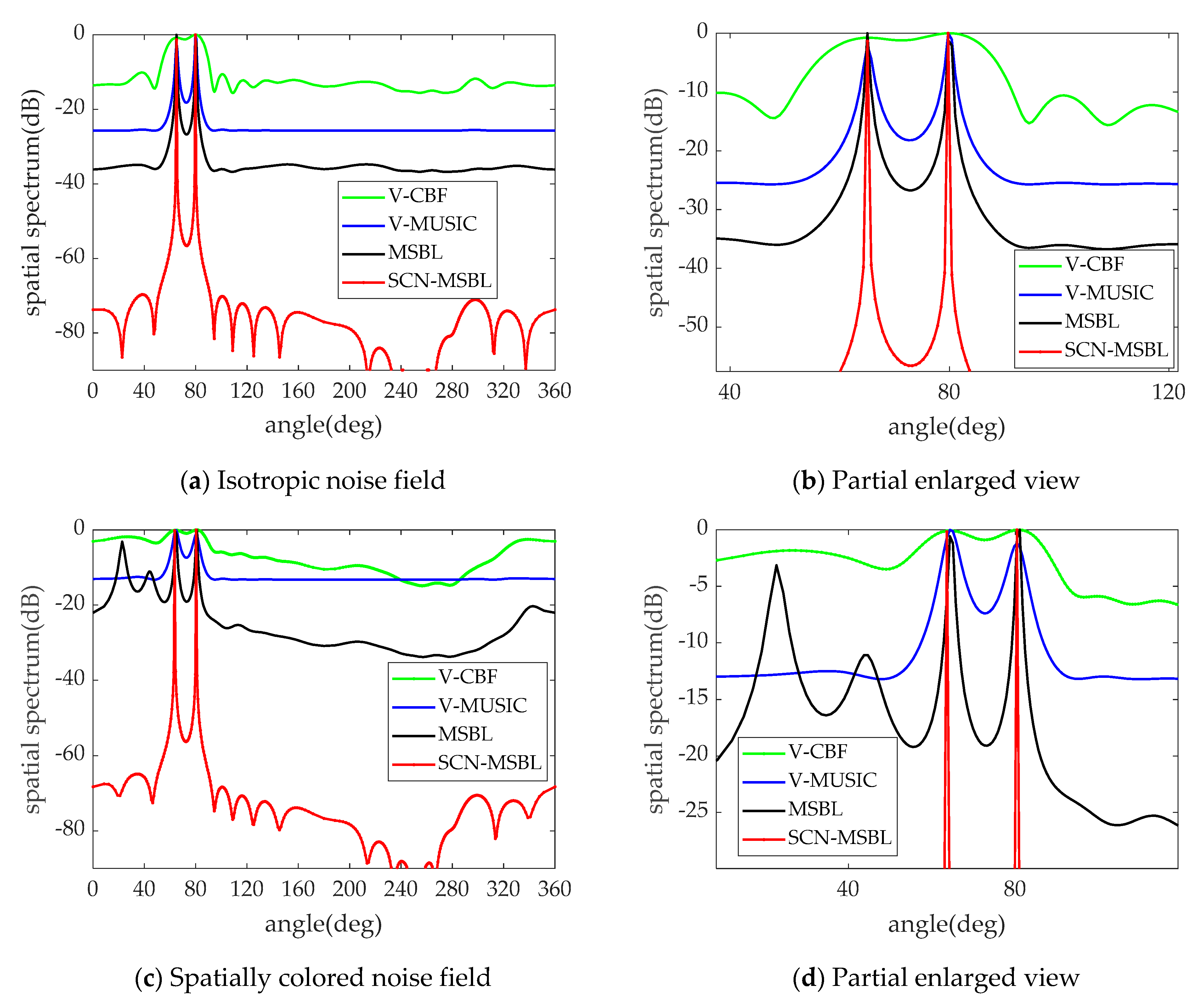
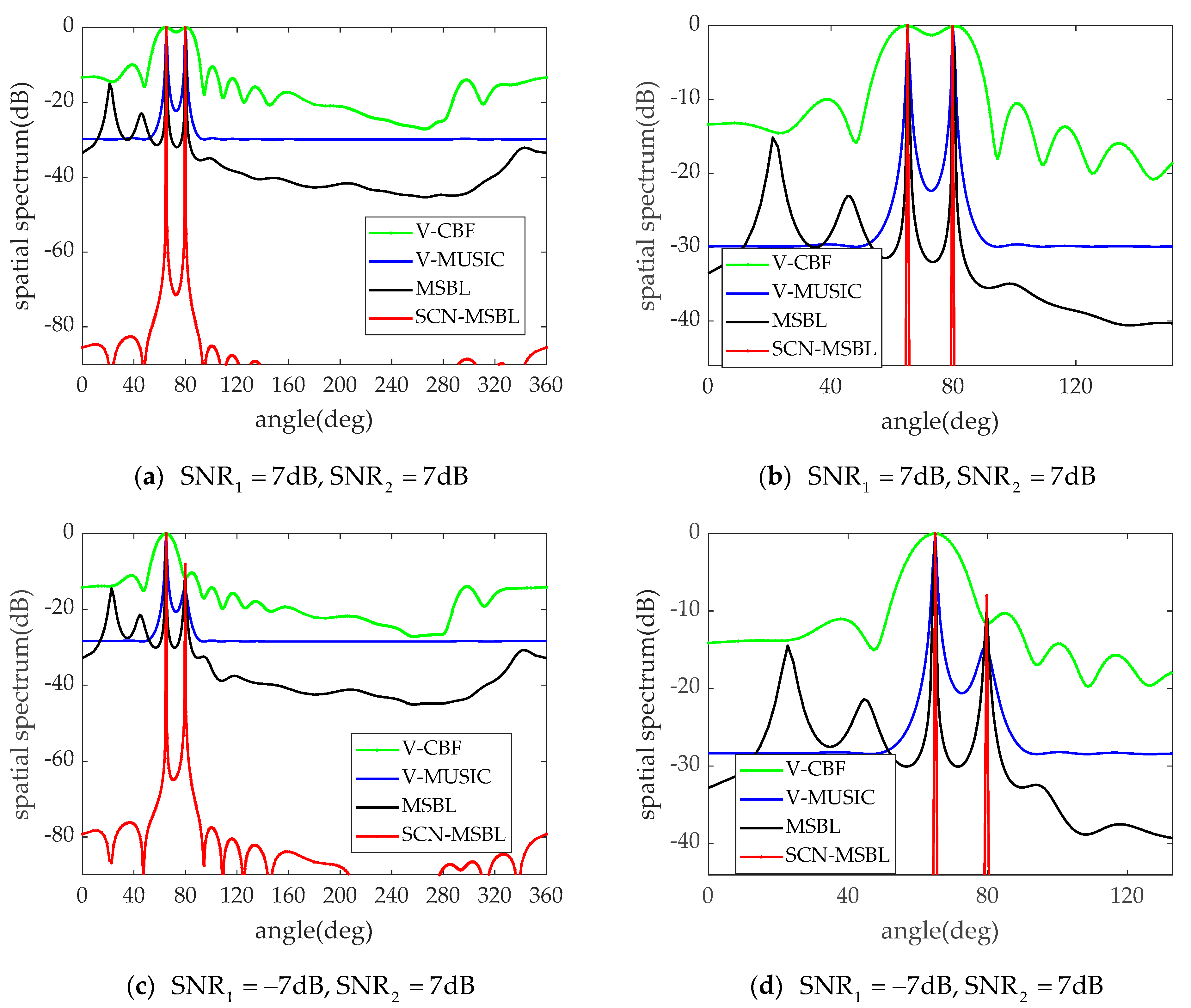
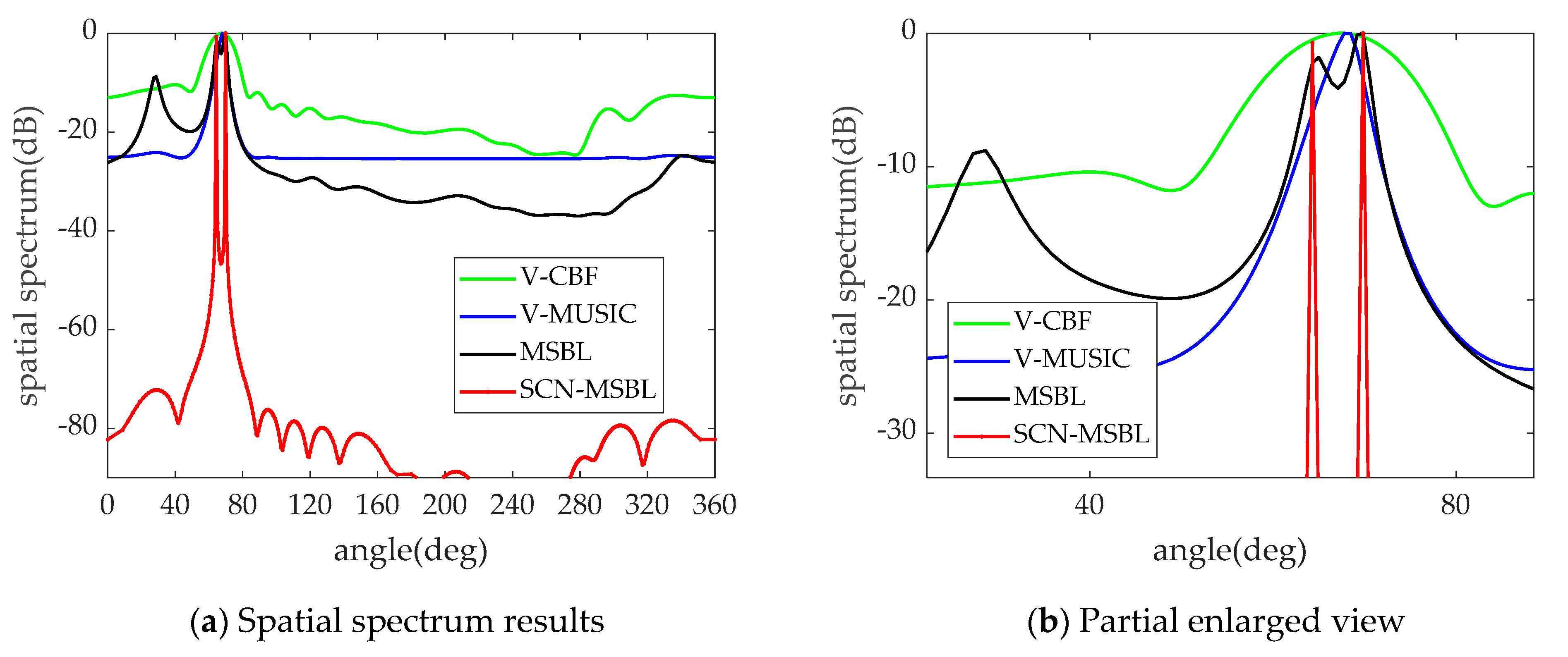
4.1. Simulation Results of Spatial Spectrum Estimates

Firstly, we discuss the effect of spatially colored noise on different algorithms from the perspective of spatial spectral estimation. It is assumed that two spatially uncorrelated far-field narrowband signals are incident on the vector hydrophone array from 65° and 80° with equal power. The number of snapshots is 200. The noise field is constructed using the numerical simulation method introduced in Section 2. Figure 4 shows the probability density functions of the spatial distribution of noise sources in an isotropic noise field as well as in a spatially inhomogeneous noise field. In the simulated isotropic noise field, the numerically constructed noise sources are uniformly distributed in all directions in space, as shown by the solid line in the figure. The spatially colored noise field shown by the dashed line has obvious spatial directionality, with the noise intensity significantly higher in a larger range near 60° than in other directions.

Figure 5 shows the spatial spectrum estimation results of the V-CBF, V-MUSIC, MSBL and SCN-MSBL, when two sources are incident on the array with $\mathrm{SNR}=-7\mathrm{dB}$. Figure 5b,d are partial enlarged views. As can be seen in Figure 5a,b, several algorithms are able to obtain accurate DOA estimates in an isotropic noise environment, and the noise spectrum far away from the signal is flatter. Among them, the CBF algorithm has the weakest resolving ability and the highest noise spectral level. The V-MUSIC algorithm has a sharper spectral peak because it exploits the orthogonality between the signal and noise subspaces, but not as sharp as the MSBL algorithm and the proposed algorithm. The reason is that the latter two take into account the potential sparsity properties in the signal model. Comparing Figure 5a,c, it can be seen that the V-CBF, V-MUSIC, and MSBL algorithms are all affected by the spatially colored noise to different degrees. Specifically, the noise spectrum of the V-CBF algorithm in the colored noise field is jittered and the spectral level is raised, which is not conducive to distinguishing the real signal. Meanwhile the noise spectrum obtained by the V-MUSIC algorithm is still flat, but the spectral level is also raised, and the spectral peak corresponding to the real signal position is wider. The MSBL algorithm is still able to output sharper spectral peaks at the true position of the signal, but it outputs more pseudo-peaks under the influence of colored noise fields; these performance degradations are caused by the noise model mismatch, while the SCN-MSBL algorithm proposed in this paper is able to adapt to the negative effects of the spatial directionality of the noise because it constructs a new linear model for spatially colored noise fields. As can be seen in Figure 5, the SCN-MSBL algorithm takes into account the noise model and the sparse characteristics of the signal in the space domain, so the accuracy and resolution of the DOA estimation are guaranteed.

Next, we change the SNR of the two spatial sources and observe the spatial spectrum estimation results of the algorithms when the target strength is obvious. The environmental noise is the spatially colored noise field shown by the dotted line in Figure 4, and the other simulation conditions remain unchanged. Figure 6 shows the spatial spectrum of the four algorithms for DOA estimation. The SNRs of the two sources in Figure 6a are both $7\hspace{0.17em}\mathrm{dB}$, and Figure 6b is a partial enlarged view. In Figure 6c, the SNR of the source at 65° is $7\hspace{0.17em}\mathrm{dB}$, and the SNR at 80° is $-\hspace{0.17em}7\mathrm{dB}$. Similarly, Figure 6d is the partial enlarged view. Comparing Figure 5c,d with Figure 6a,b, it can be seen that, as the input SNR increases, the performance of each algorithm improves to a certain extent. Although the MSBL algorithm is still affected by some false peaks, their height is relatively low, so it can find the real target location correctly. When two spatial targets, one strong and one weak, are incident on the array (as shown in Figure 6c,d), it is difficult to find the position of the weak target in the spatial spectrum obtained by the V-CBF algorithm. The MSBL algorithm cannot eliminate the influence of false peaks because the height of the false peak is close to the peak value of the weak target. However, the proposed algorithm uses a more extensive noise model and has stronger adaptability to the spatial distribution of noise. Therefore, the performance is very robust under various SNRs and noise background types, bring the sharpest peaks. It is worth noting that although the V-MUSIC algorithm can output the true position relatively stably under various simulation conditions. However, the accurate distinction between signal and noise subspaces is based on the premise that the number of independent sources is known a priori. The algorithm in this paper does not require the number of sources as a priori input, and the sharpness of the spectral peak is much better than other algorithms.

Continue to reduce the interval between the incident angles of the sources, and the two sources are incident from 65° and 70° respectively. The SNR and the number of snapshots is $0\hspace{0.17em}\mathrm{dB}$ and 200, respectively. The spatial spectrum result is shown in Figure 7.

As can be seen from Figure 7, when the two targets differ by only 5°, V-CBF and V-MUSIC can no longer distinguish the two targets at all. MSBL can barely distinguish the two targets although it has the highest resolution capability of the sparse reconstruction algorithm, but the DOA estimation results deviate to some extent from the true results and are seriously affected by the pseudo-peak problem. Only the proposed algorithm can accurately estimate the true angles of two adjacent targets. The above simulations show that the accuracy and resolving ability of the SCN-MSBL algorithm in DOA estimation under spatially colored noise are higher than those of other algorithms.

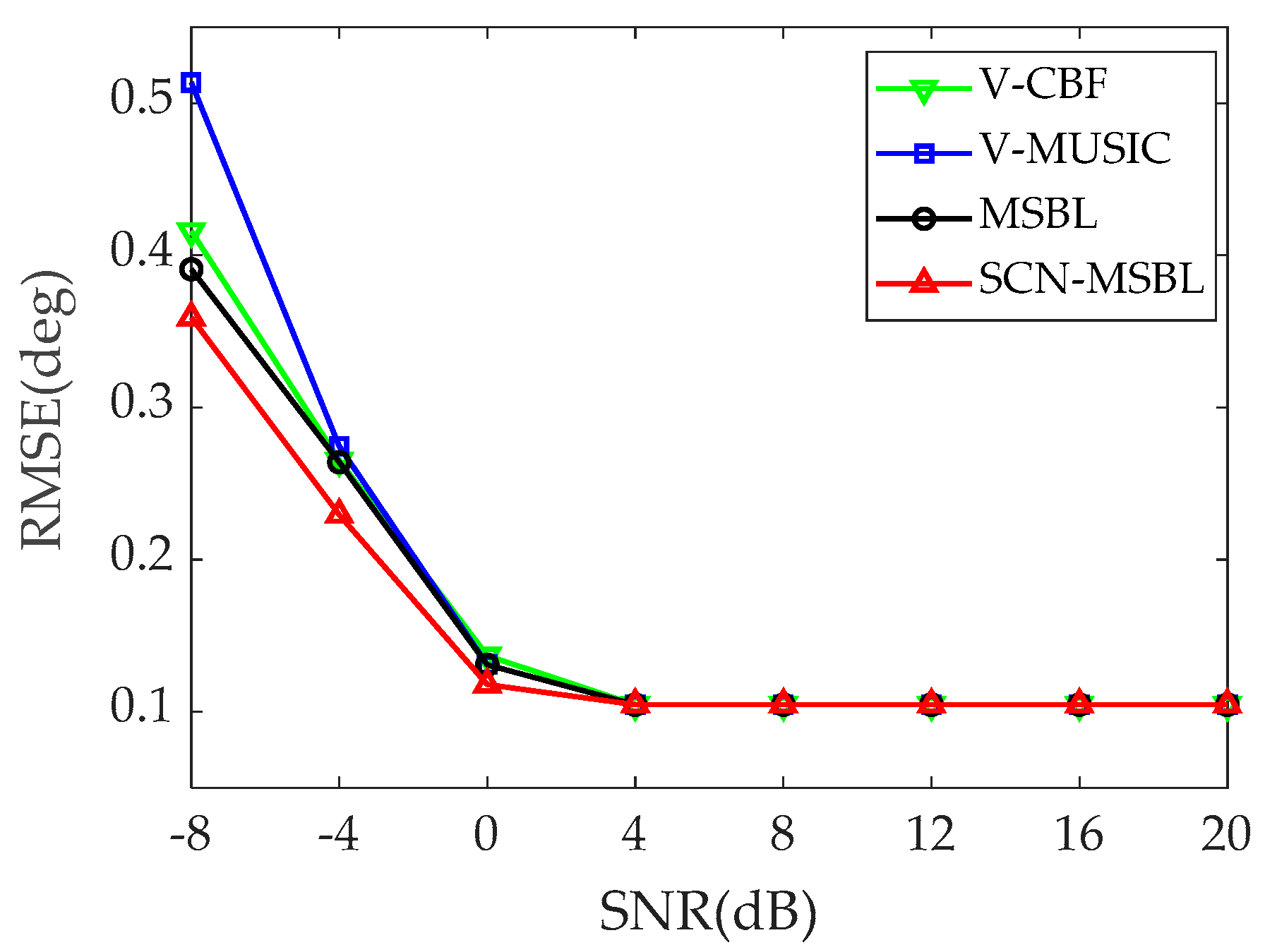
4.2. Statistical Performance Analysis of Simulation Results

In order to obtain this statistical performance more accurately, the two far-field signals used in this simulation were oriented at 70.1° and 90.9°, to ensure that all algorithms were able to distinguish between the two sources and thus obtain more accurate statistical results. The SNR was varied from $-8\hspace{0.17em}\mathrm{dB}$ to $20\hspace{0.17em}\mathrm{dB}$, and 200 Monte Carlo trials were performed in each SNR case with a snapshot number of 200 and the same spatially colored noise distribution as in Experiment 1.

The statistical results are given in Figure 8. It can be seen that, at low SNRs, the SCN-MSBL algorithm has the highest accuracy and the V-MUSIC algorithm has the lowest estimation accuracy. As the SNR increases, all methods maintain the high estimation accuracy. The DOA estimates obtained by the sparse reconstruction method still fall on the nearest raster point to the true DOA, even if the spatial grid division does not pick up the true position of the signal. Due to the effect of quantization error, the root mean square error (RMSE) of the DOA estimate does not continue to decrease as the SNR increases, but rather plateaus. In the practical application of the algorithm, a strategy of grid refinement or a strategy of discrete grids [44] can be used to further reduce the effect of quantization error.

Next, fixing the SNR as $0\hspace{0.17em}\mathrm{dB}$, the variation of the RMSE with the number of snapshots was analysed. The results are shown in Figure 9. It can be seen that the RMSE of DOA estimation gradually decreases as the number of snapshots increases. The estimation accuracy tends to smooth out when the number of snapshots is large enough for the quantization error to play a dominant role. In addition, when the azimuth of the space target is far apart, except for the poor estimation accuracy of the V-CBF algorithm in small snapshots, the DOA estimation performance of the other algorithms is relatively close, and the performance of the DN-MSBL algorithm is slightly better than the other algorithms.

The ability of each algorithm to discriminate between adjacent targets was examined by means of Monte Carlo tests. Firstly, the two targets in space are made to be incident on the array from 70° and 75° respectively. The SNR is varied from $-8\hspace{0.17em}\mathrm{dB}$ to $20\hspace{0.17em}\mathrm{dB}$. 200 Monte Carlo trials were performed in each SNR case with a snapshot number of 200. The results to determine whether the algorithms could successfully discriminate between the two targets are shown in Figure 10.

As can be seen from the Figure 10, in the range of SNRs of the simulation, the V-CBF algorithm is always unable to resolve two targets with an angle interval of 5°. The probability of successful resolution of the remaining methods increases with the increase of the SNR. When SNR is higher than $8\hspace{0.17em}\mathrm{dB}$, all the algorithms except the V-CBF algorithm are able to resolve the dual targets with 100% probability. Besides, the MSBL and the SCN-MSBL algorithm have a higher resolution capability than the classical high-resolution algorithm (V-MUSIC) due to the constraint on the sparsity of the spatial domain of the signal. The SCN-MSBL algorithm has the lowest SNR threshold required to successfully resolve the dual targets with 100% probability, which is about $-4\hspace{0.17em}\mathrm{dB}$.

Finally, we fix the incidence angle of source 1 at 70° and make the incidence angle of source 2 vary from 72° to 90° to gives the variation of the successful resolution probability for the four algorithms. Figure 11 shows the results when the SNR is $0\hspace{0.17em}\mathrm{dB}$ and the number of snapshots is 200. It can be seen that the resolution capability of the V-CBF algorithm is the worst, and the resolution ability of the SCN-MSBL and the MSBL algorithm is the strongest, while the SCN-MSBL algorithm has a smaller angle interval threshold. Therefore, using the noise model described in this paper, combined with the spatial sparsity constraint, we can distinguish adjacent targets better, which also verifies the conclusions of the resolution ability of each algorithm in Experiment 1.

We provide a comparison table which clearly states the differences of the proposed algorithm and other algorithms mentioned in this paper. The table is as

Table 1. Comparison Table.

Approach	Advantages	Disadvantages
V-CBF	Noise robustness	Poor resolution
	Faster and low complexity	Not suitable for spatially colored noise
V-MUSIC	Ability to super-resolve	Not suitable for spatially colored noise
MSBL	Higher resolution capability	High computational cost
	Higher estimation accuracy	Results are prior dependent which is needed to select
		Not suitable for spatially colored noise
SCN-MSBL	Higher resolution capability	High computational cost
	Higher estimation accuracy	Results are prior dependent which is needed to select
	Suitable for spatially colored noise

:

5. Conclusions

Many high-resolution DOA estimation algorithms achieve very good performance under the isotropic Gaussian noise background. However, the presence of wind and waves, distant travelling vessels and local platform noise often makes the noise received by the array directional. This paper first introduces the volume noise model and the numerical simulation method, then analyses the effect of near-field volume noise on the spatial spectrum. It has been found that the noise spatial spectrum of the vector hydrophone array has certain directivity under the influence of near-field volume noise. To solve this problem, we present the excellent characteristics of the PSWFs for fitting finite bandwidth signals, and extends this feature to the spatial domain. A linear model of spatially colored noise is constructed based on the analogous properties of time domain sampling and spatial sampling. Using the sparsity of the proposed noise model and the signal in the spatial domain, the overcomplete model of the array output is established. As a result, the sparse Bayesian learning technique is introduced in the DOA estimation process. It makes full use of the multi-level probability model of the sparse Bayesian learning method to jointly and iteratively obtain the noise parameters and the signal reconstruction. The reconstruction accuracy of the algorithm is improved under spatially colored noise field. Simulation experiments demonstrate the effectiveness of this method in different noise environments.

The theoretical and simulation analyses show that the SCN-MSBL algorithm proposed in this paper has the following features and advantages.

(1)

When the spatial noise is highly directional, the proposed algorithms effectively suppress the significant increase in pseudo-peaks and noise spectral levels, while ensuring the high resolution of the sparse reconstruction class algorithm.

(2)

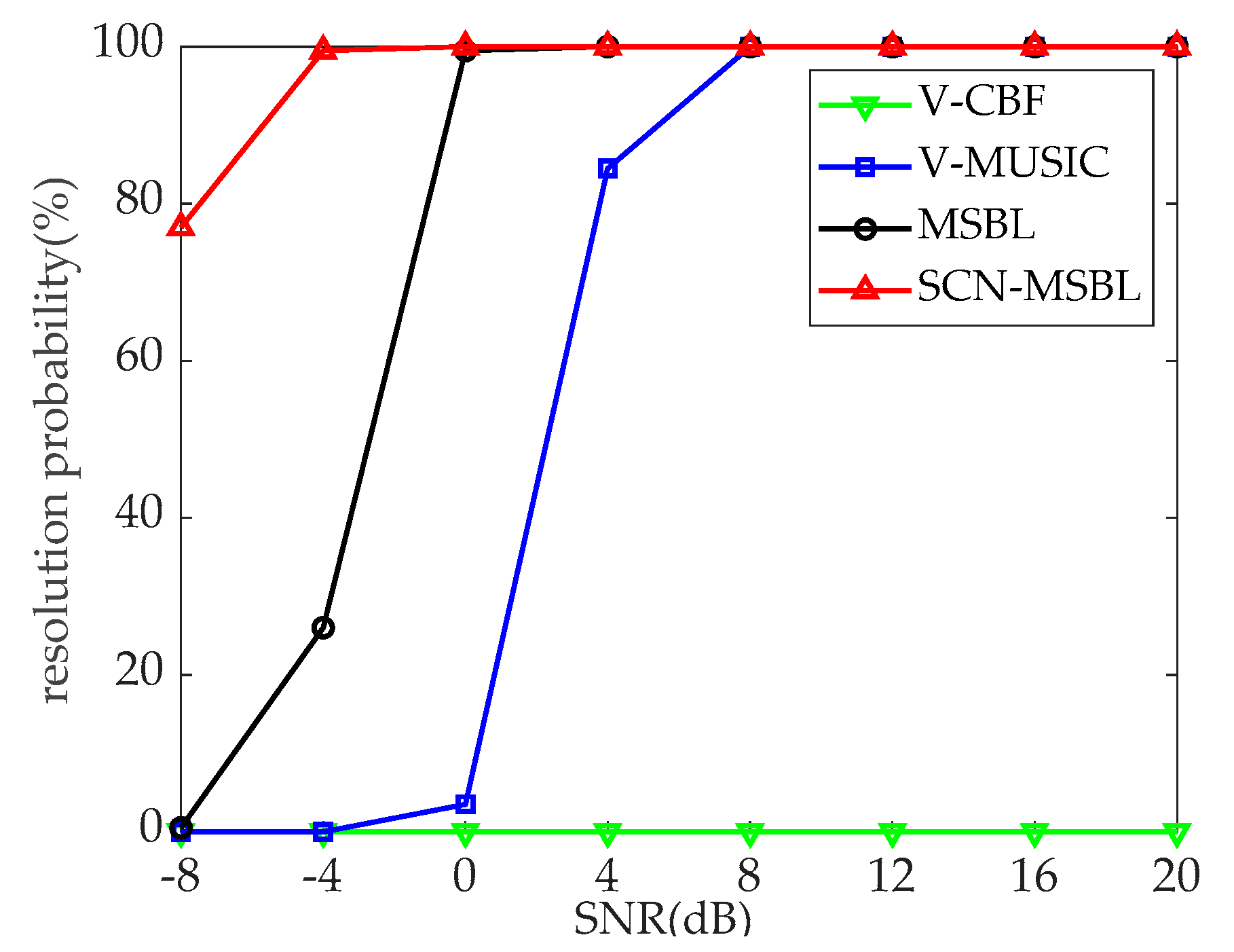
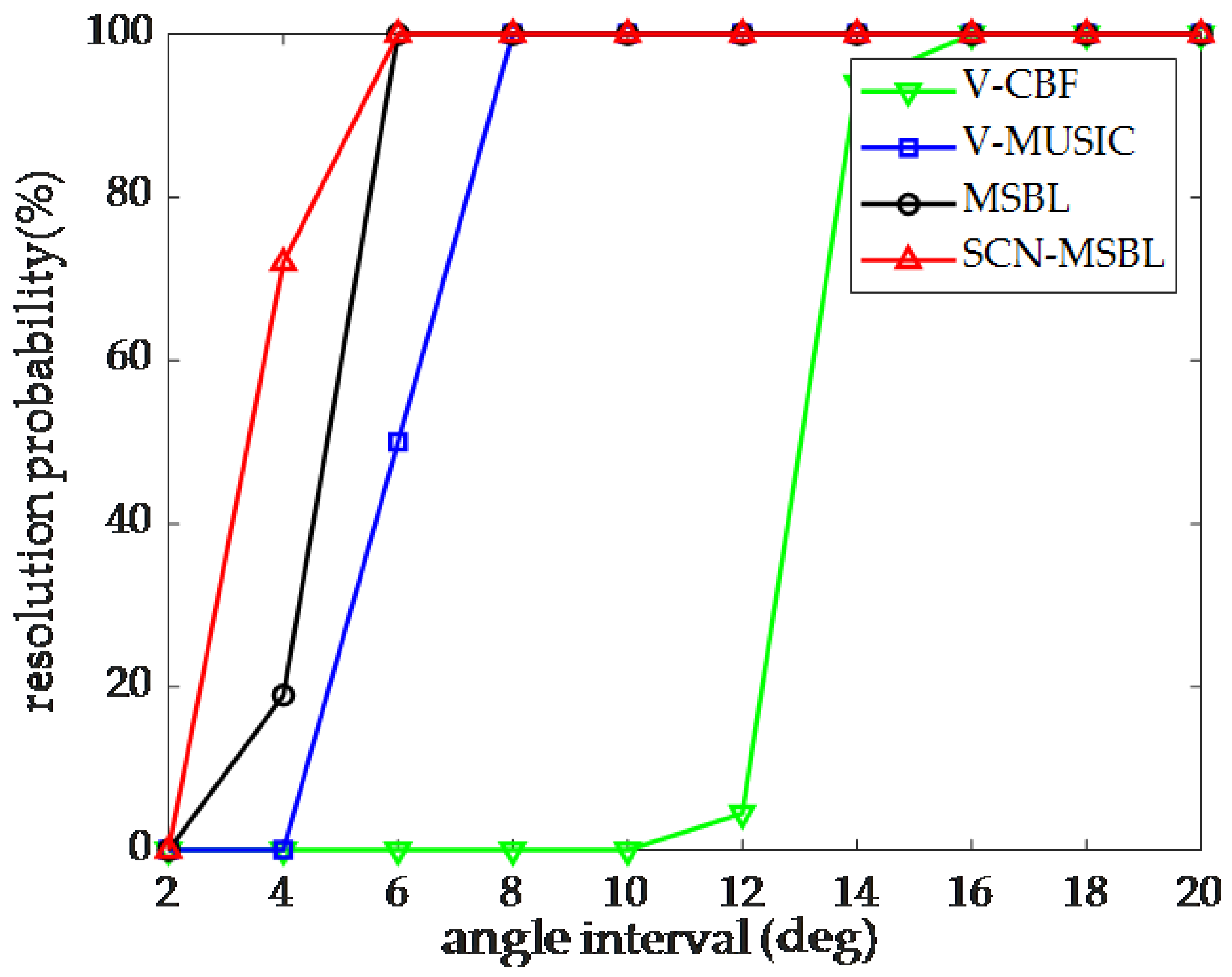
The proposed algorithms require lower SNR thresholds and angle interval thresholds to successfully distinguish adjacent targets, compared to beamforming algorithms and subspace-like algorithms.

(3)

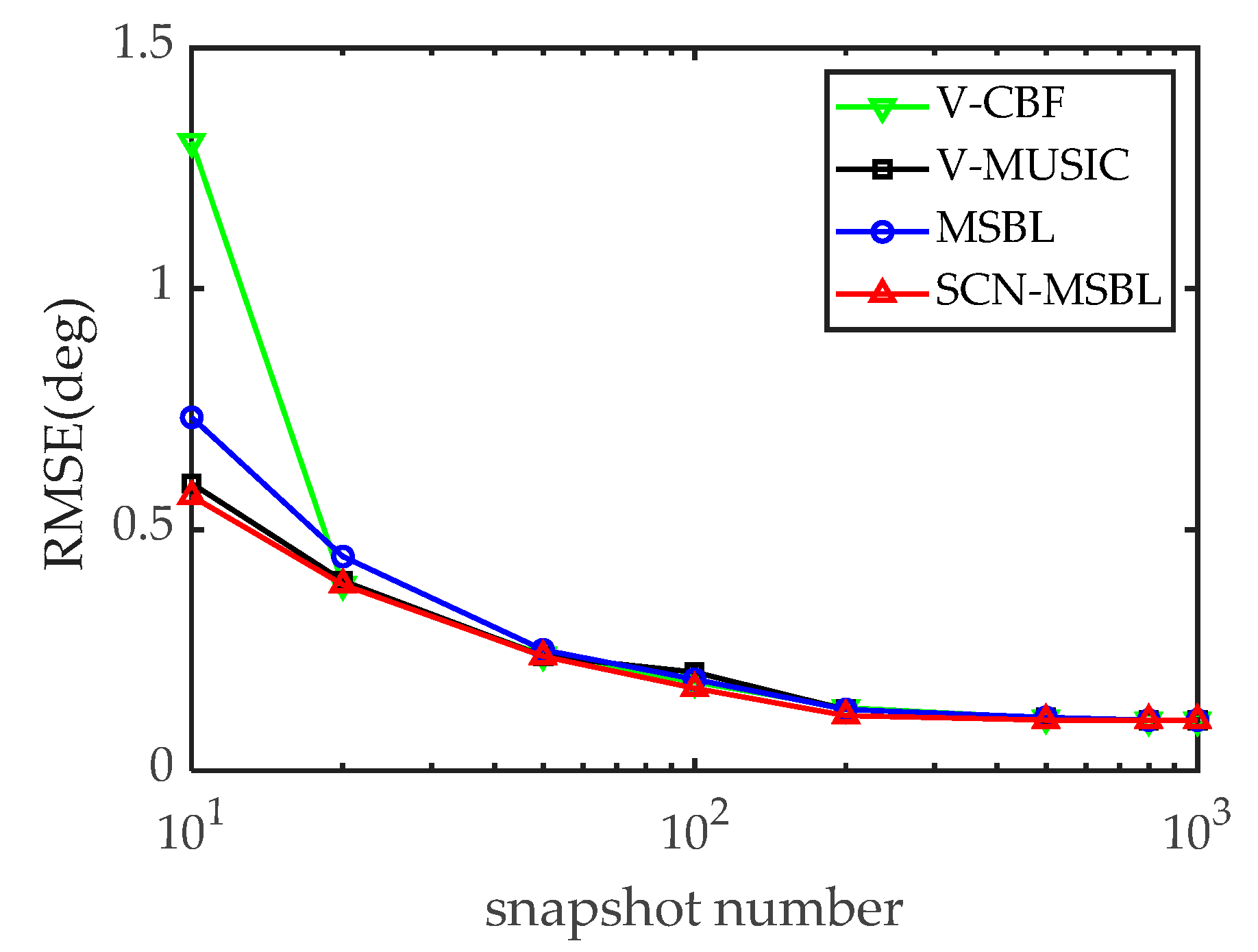
As for the accuracy of the DOA estimation, the RMSE of the DOA estimation of the SCN-MSBL algorithm is slightly smaller than that of the V-MUSIC algorithm, and comparable to that of the MSBL algorithm, provided that all methods can accurately distinguish the adjacent targets.

The sparse reconstruction-type DOA estimation algorithm exploits the sparse spatial characteristics of the source. It transforms the DOA estimation problem into a sparse reconstruction problem by building an overcomplete model of the array output signal, achieving a very high resolution. However, in the spatially colored noise environment, the sparse reconstruction algorithm is prone to pseudo-peaks and even failure. The algorithm proposed in this paper not only makes full use of the advantages of the sparse reconstruction class algorithm, but also refines the spatially colored noise model. Besides, the proposed algorithm obtains higher resolution, estimation accuracy, and better noise robustness, laying the foundation for subsequent research on array signal processing using the framework of sparse reconstruction. The main disadvantage of the proposed method is the large amount of computation, so our next objective is to develop a fast algorithm to facilitate the real-time operation of this method.

References

1. Shi, Z.; Liang, G.; Qiu, L.; Wan, G.; Zhao, L. Vector Hydrophone Array Design Based on Off-Grid Compressed Sensing. Sensors 2020, 20, 6949. [Google Scholar] [CrossRef]
2. Nehorai, A.; Paldi, E. Acoustic vector-sensor array processing. IEEE Trans. Signal Process. 1994, 42, 2481–2491. [Google Scholar] [CrossRef]
3. Chen, H.-W.; Zhao, J.-W. Wideband MVDR beamforming for acoustic vector sensor linear array. IEEE Proc. Radar. Sonar Navig. 2004, 151, 158. [Google Scholar] [CrossRef]
4. Wong, K.; Zoltowski, M. ESPRIT-based extended-aperture source localization using velocity-hydrophones. In OCEANS 96 MTS/IEEE Conference, Proceedings of the Coastal Ocean Prospects for the 21st Century, Fort Lauderdale, FL, USA, 23–26 September 1996; IEEE: Piscataway, NJ, USA, 2002; Volume 3, pp. 1427–1432. [Google Scholar]
5. Wong, K.; Zoltowski, M. Extended-aperture underwater acoustic multisource azimuth/elevation direction-finding using uniformly but sparsely spaced vector hydrophones. IEEE J. Ocean. Eng. 1997, 22, 659–672. [Google Scholar] [CrossRef]
6. Wong, K.T.; Zoltowski, M.D. Polarization-beamspace self-initiating MUSIC for azimuth/elevation angle estimation. In Proceedings of the Radar Systems (RADAR 97), Edinburgh, UK, 14–16 October 1997; pp. 328–333. [Google Scholar]
7. Hamson, R. The modelling of ambient noise due to shipping and wind sources in complex environments. Appl. Acoust. 1997, 51, 251–287. [Google Scholar] [CrossRef]
8. Sabra, K.; Roux, P.; Thode, A.; D’Spain, G.; Hodgkiss, W.; Kuperman, W. Using Ocean Ambient Noise for Array Self-Localization and Self-Synchronization. IEEE J. Ocean. Eng. 2005, 30, 338–347. [Google Scholar] [CrossRef]
9. Shi, Y.; Yang, Y.; Tian, J.; Sun, C.; Zhao, W.; Li, Z.; Ma, Y. Long-term ambient noise statistics in the northeast South China Sea. J. Acoust. Soc. Am. 2019, 145, EL501–EL507. [Google Scholar] [CrossRef] [Green Version]
10. Huang, Y.; Guo, J. Spatial correlation of the acoustic vector field of the surface noise in three-dimensional ocean environments. J. Acoust. Soc. Am. 2014, 135, 2397. [Google Scholar] [CrossRef]
11. Cron, B.F.; Sherman, C.H. Spatial-Correlation Functions for Various Noise Models. J. Acoust. Soc. Am. 1962, 34, 1732–1736. [Google Scholar] [CrossRef]
12. Wang, Y.; Yang, Y.; He, Z.; Ma, Y.; Li, B. Robust Superdirective Frequency-Invariant Beamforming for Circular Sensor Arrays. IEEE Signal Process. Lett. 2017, 24, 1193–1197. [Google Scholar] [CrossRef]
13. Shchurov, V.A. Coherent and diffusive fields of underwater acoustic ambient noise. J. Acoust. Soc. Am. 1991, 90, 991–1001. [Google Scholar] [CrossRef]
14. Hawkes, M.; Nehorai, A. Acoustic vector-sensor correlations in ambient noise. IEEE J. Ocean. Eng. 2001, 26, 337–347. [Google Scholar] [CrossRef] [Green Version]
15. Viberg, M. Sensitivity of parametric direction finding to colored noise fields and undermodeling. Signal Process. 1993, 34, 207–222. [Google Scholar] [CrossRef]
16. Li, M.; Lu, Y. Dimension reduction for array processing with robust interference cancellation. IEEE Trans. Aerosp. Electron. Syst. 2006, 42, 103–112. [Google Scholar] [CrossRef]
17. Meng, Z.; Shen, F.; Zhou, W. Adaptive beamforming using the cyclostationarity of the source signals. Electron. Lett. 2017, 53, 858–860. [Google Scholar] [CrossRef]
18. Meng, Z.; Shen, F.; Zhou, W. Iterative adaptive approach to interference covariance matrix reconstruction for robust adaptive beamforming. IET Microwaves Antennas Propag. 2018, 12, 1704–1708. [Google Scholar] [CrossRef]
19. Meng, Z.; Zhou, W. Robust adaptive beamforming using iterative adaptive approach. J. Electromagn. Waves Appl. 2018, 33, 504–519. [Google Scholar] [CrossRef]
20. Meng, Z.; Zhou, W. Direction-of-Arrival Estimation in Coprime Array Using the ESPRIT-Based Method. Sensors 2019, 19, 707. [Google Scholar] [CrossRef] [Green Version]
21. Sun, S.; Zhang, X.; Zheng, C.; Fu, J.; Zhao, C. Underwater Acoustical Localization of the Black Box Utilizing Single Autonomous Underwater Vehicle Based on the Second-Order Time Difference of Arrival. IEEE J. Ocean. Eng. 2020, 45, 1268–1279. [Google Scholar] [CrossRef]
22. Sun, S.; Qin, S.; Hao, Y.; Zhang, G.; Zhao, C. Underwater Acoustic Localization of the Black Box Based on Generalized Second-Order Time Difference of Arrival (GSTDOA). IEEE Trans. Geosci. Remote. Sens. 2020, 1–11. [Google Scholar] [CrossRef]
23. Xie, J.; Yuan, Y.; Liu, Y. Super-resolution processing for HF surface wave radar based on pre-whitened MUSIC. IEEE J. Ocean. Eng. 1998, 23, 313–321. [Google Scholar] [CrossRef]
24. Wu, Y.; Hou, C.; Liao, G.; Guo, Q. Direction-of-Arrival Estimation in the Presence of Unknown Nonuniform Noise Fields. IEEE J. Ocean. Eng. 2006, 31, 504–510. [Google Scholar] [CrossRef] [Green Version]
25. Le Cadre, J. Parametric methods for spatial signal processing in the presence of unknown colored noise fields. IEEE Trans. Acoust. Speech Signal Process. 1989, 37, 965–983. [Google Scholar] [CrossRef] [Green Version]
26. Tewfik, A. Direction finding in the presence of colored noise by candidate identification. IEEE Trans. Signal Process. 1991, 39, 1933–1942. [Google Scholar] [CrossRef]
27. Ye, H.; DeGroat, D. Maximum likelihood DOA estimation and asymptotic Cramer-Rao bounds for additive unknown colored noise. IEEE Trans. Signal Process. 1995, 43, 938–949. [Google Scholar] [CrossRef]
28. Nagesha, V.; Kay, S. Maximum likelihood estimation for array processing in colored noise. IEEE Trans. Signal Process. 1996, 44, 169–180. [Google Scholar] [CrossRef]
29. Tugnait, J. Time delay estimation with unknown spatially correlated Gaussian noise. IEEE Trans. Signal Process. 1993, 41, 549–558. [Google Scholar] [CrossRef]
30. Cardoso, J.-F.; Moulines, E. Asymptotic performance analysis of direction-finding algorithms based on fourth-order cumulants. IEEE Trans. Signal Process. 1995, 43, 214–224. [Google Scholar] [CrossRef] [Green Version]
31. Paulraj, A.; Kailath, T. Eigenstructure methods for direction of arrival estimation in the presence of unknown noise fields. IEEE Trans. Acoust. Speech Signal Process. 1986, 34, 13–20. [Google Scholar] [CrossRef]
32. Jin, M.; Liao, G.; Li, J. Joint DOD and DOA estimation for bistatic MIMO radar. Signal Process. 2009, 89, 244–251. [Google Scholar] [CrossRef]
33. Chen, J.; Gu, H.; Su, W. A new method for joint DOD and DOA estimation in bistatic MIMO radar. Signal Process. 2010, 90, 714–718. [Google Scholar] [CrossRef]
34. Wen, F.; Xiong, X.; Su, J.; Zhang, Z. Angle estimation for bistatic MIMO radar in the presence of spatial colored noise. Signal Process. 2017, 134, 261–267. [Google Scholar] [CrossRef]
35. Wen, F.; Zhang, Z.; Zhang, G. Joint DOD and DOA Estimation for Bistatic MIMO Radar: A Covariance Trilinear Decomposition Perspective. IEEE Access 2019, 7, 53273–53283. [Google Scholar] [CrossRef]
36. Hong, S.; Wan, X.; Cheng, F.; Ke, H. Covariance differencing-based matrix decomposition for coherent sources localisation in bi-static multiple-input-multiple-output radar. IET Radar Sonar Navig. 2015, 9, 540–549. [Google Scholar] [CrossRef]
37. He, J.; Liu, Z. Two-dimensional direction finding of acoustic sources by a vector sensor array using the propagator method. Signal Process. 2008, 88, 2492–2499. [Google Scholar] [CrossRef]
38. Qiu, L.; Lan, T.; Wang, Y. A Sparse Perspective for Direction-of-Arrival Estimation Under Strong Near-Field Interference Environment. Sensors 2019, 20, 163. [Google Scholar] [CrossRef] [Green Version]
39. Wang, L.; Zhao, L.; Bi, G.; Wan, C.; Zhang, L.; Zhang, H. Novel Wideband DOA Estimation Based on Sparse Bayesian Learning with Dirichlet Process Priors. IEEE Trans. Signal Process. 2015, 64, 275–289. [Google Scholar] [CrossRef]
40. Yang, Z.; Xie, L.; Zhang, C. Off-Grid Direction of Arrival Estimation Using Sparse Bayesian Inference. IEEE Trans. Signal Process. 2013, 61, 38–43. [Google Scholar] [CrossRef] [Green Version]
41. Liu, H.; Zhao, L.; Li, Y.; Jing, X.; Truong, T.-K. A Sparse-Based Approach for DOA Estimation and Array Calibration in Uniform Linear Array. IEEE Sens. J. 2016, 16, 6018–6027. [Google Scholar] [CrossRef]
42. Xu, X.; Wei, X.; Ye, Z. DOA Estimation Based on Sparse Signal Recovery Utilizing Weighted l1-Norm Penalty. IEEE Signal Process. Lett. 2012, 19, 155–158. [Google Scholar] [CrossRef]
43. Zhang, Z.; Rao, B.D. Sparse Signal Recovery with Temporally Correlated Source Vectors Using Sparse Bayesian Learning. IEEE J. Sel. Top. Signal Process. 2011, 5, 912–926. [Google Scholar] [CrossRef] [Green Version]
44. Malioutov, D.; Cetin, M.; Willsky, A. A sparse signal reconstruction perspective for source localization with sensor arrays. IEEE Trans. Signal Process. 2005, 53, 3010–3022. [Google Scholar] [CrossRef] [Green Version]
45. Wang, Y.; Yang, X.; Xie, J.; Wanga, L.; Ng, B.W.-H. Sparsity-Inducing DOA Estimation of Coherent Signals Under the Coexistence of Mutual Coupling and Nonuniform Noise. IEEE Access 2019, 7, 40271–40278. [Google Scholar] [CrossRef]
46. Hu, N.; Sun, B.; Zhang, Y.; Dai, J.; Wang, J.; Chang, C. Underdetermined DOA Estimation Method for Wideband Signals Using Joint Nonnegative Sparse Bayesian Learning. IEEE Signal Process. Lett. 2017, 24, 535–539. [Google Scholar] [CrossRef]
47. Friedlander, B.; Weiss, A. Direction finding using noise covariance modeling. IEEE Trans. Signal Process. 1995, 43, 1557–1567. [Google Scholar] [CrossRef]
48. Landau, H.J.; Pollak, H.O. Prolate spheroidal wave functions, Fourier analysis and uncertainty principle II. Bell System Tech. J. 1961, 40, 65–84. [Google Scholar] [CrossRef]
49. Slepian, D.; Pollak, H.O. Prolate Spheroidal Wave Functions, Fourier Analysis and Uncertainty I. Bell Syst. Tech. J. 1961, 40, 43–63. [Google Scholar] [CrossRef]
50. Xiao, H.; Rokhlin, V.; Yarvin, N. Prolate spheroidal wavefunctions, quadrature and interpolation. Inverse Probl. 2001, 17, 805–838. [Google Scholar] [CrossRef]
51. Chen, C.-Y.; Vaidyanathan, P.P. MIMO Radar Space–Time Adaptive Processing Using Prolate Spheroidal Wave Functions. IEEE Trans. Signal Process. 2008, 56, 623–635. [Google Scholar] [CrossRef]
52. Slepian, D. Prolate Spheroidal Wave Functions, Fourier Analysis, and Uncertainty-V: The Discrete Case. Bell Syst. Tech. J. 1978, 57, 1371–1430. [Google Scholar] [CrossRef]
53. Scheinman, A.H. A Method for Simplifying Boolean Functions. Bell Syst. Tech. J. 1962, 41, 1337–1346. [Google Scholar] [CrossRef]
54. Gosse, L. Effective band-limited extrapolation relying on Slepian series and ℓ1 regularization. Comput. Math. Appl. 2010, 60, 1259–1279. [Google Scholar] [CrossRef] [Green Version]
55. Shkolnisky, Y.; Tygert, M.; Rokhlin, V. Approximation of bandlimited functions. Appl. Comput. Harmon. Anal. 2006, 21, 413–420. [Google Scholar] [CrossRef] [Green Version]
56. Wang, L.-L. Analysis of spectral approximations using prolate spheroidal wave functions. Math. Comput. 2009, 79, 807–827. [Google Scholar] [CrossRef] [Green Version]
57. Walden, A.T. Spectral Analysis for Physical Applications; Cambridge University Press: Cambridge, UK, 1993. [Google Scholar]
Figure 1. Acoustic vector sensor correlations in ambient noise.
Jmse 09 00127 g001
Figure 2. Spatial spectrum under isotropic noise.
Jmse 09 00127 g002
Figure 3. Spatial spectrum under spatially colored noise.
Jmse 09 00127 g003
Figure 4. Spatial probability density distribution of numerical noise sources.
Jmse 09 00127 g004
Figure 5. Influence of directional noise on spatial spectrum. (a) Isotropic noise field, (b) Partial enlarged view, (c) Spatially colored noise field, (d) Partial enlarged view.
Jmse 09 00127 g005
Figure 6. Spatial spectrum under directional noise field. (a) SNR 1 = 7 dB , SNR 2 = 7 dB , (b) SNR 1 = 7 dB , SNR 2 = 7 dB , (c) SNR 1 = 7 dB , SNR 2 = 7 dB , (d) SNR 1 = 7 dB , SNR 2 = 7 dB .
Jmse 09 00127 g006
Figure 7. Spatial spectrum of two closed sources. (a) Spatial spectrum results, (b) Partial enlarged view.
Jmse 09 00127 g007
Figure 8. RMSE of direction-of-arrival (DOA) estimation versus signal-to-noise (SNR).
Jmse 09 00127 g008
Figure 9. The variation of the RMSE with the number of snapshots.
Jmse 09 00127 g009
Figure 10. RMSE of DOA estimation versus snapshots.
Jmse 09 00127 g010
Figure 11. Resolution probabilities of different methods versus SNR.
Jmse 09 00127 g011