Abstract
Velocity is vital information for navigation and oceanic engineering. Coherent Doppler sonar is an accurate tool for velocity measurement, but its use is limited due to velocity ambiguity. Velocity measured by frequency shift has no velocity ambiguity, yet its measurement error is larger than that of coherent Doppler sonar. Therefore, coherent Doppler sonar assisted by frequency shift is used to accurately measure velocity without velocity ambiguity. However, the velocity measured by coherent Doppler sonar assisted by frequency shift is affected by impulsive noise. To decrease the impulsive noise, Kalman filter and linear prediction are proposed to improve the velocity sensing accuracy. In this method, the Kalman filter is used to decrease measurement error of velocity measured by frequency shift, and linear prediction is used to remove the impulsive noise generated by a wrong estimate of the integer ambiguity. Lab-based experiments were carried, and the results have shown that coherent Doppler sonar assisted by frequency shift, Kalman filter and linear prediction can provide accurate and precise velocity with short time delay in a large range of signal to noise ratio.
1. Introduction
Velocity is vital information for ships and underwater vehicles, playing an important role in navigation and oceanic engineering. At the 2000 International Convention for the Safety of Life at Sea (SOLAS), vessels more than 50,000 gross tons were recommended to be equipped with two axes speed and distance measurement equipment (SDME) to provide velocity information [1]. In addition, there are also many benefits for navigators on the vessels less than 50,000 gross tons to use the precise velocity information. With precise velocity information, a decrease in the probability of collisions with other ships or piers and improvement of the workload safety is possible. Normally, electro-magnetic (EM) log, inertial navigation system (INS), Global Positioning System (GPS) and Doppler sonar systems are used to measure the velocity of moving vessels at sea. The EM log can only provide the velocity through water. The velocity measured by EM log is also limited to the area around the sensor. The handbook of the EM log (EML 500) indicates its accuracy as 0.1 m/s [2]. The velocity information GPS (VI-GPS) system can provide accurate velocity information relative to the earth with an accuracy of 0.01 m/s [3,4,5,6]. Unfortunately, GPS signal cannot be transmitted into water, so the VI-GPS is limited to the surface and above where it can receive the GPS signal. It also has an intrinsic disadvantage in that one of the VI-GPS sensors has to be installed on the shore of harbor. INS can also provide the velocity if the initial velocity is known, but the accumulative error seriously affects the final results. The accuracy of the INS of the Seaborne Navigation system for velocity is 0.91 m/s [7]. The Doppler sonar system can measure the velocity of objects both on the sea surface and in the water. Both the velocities relative to ground and water can be provided by the Doppler sonar system.
Conventional Doppler sonar measured velocity using frequency shift has been wildly used as a basic device installed on vessels to provide velocity information. However, the valuable reading of velocity by frequency shift in low signal to noise ratio (SNR) has a few seconds time lag [4], which is not adequate for tasks that require high velocity accuracy. Pulse-to-pulse coherent Doppler sonar (CHDS) has been developed to explore the characters of fluids, such as turbulence and wave characteristics in the ocean [8,9]. The velocity measured by CHDS is accurate over a short time lag [10,11], but the appearance of “range–velocity” ambiguity limits wider applications of CHDS. Multiple pulse repetition frequencies [12,13] and carrier frequencies [14,15] are used to enlarge the maximum measurable speed, but still the results are unsatisfactory. CHDS assisted by frequency shift (CHDSF) [16,17] was proposed to provide an accurate velocity without velocity ambiguity. However, impulsive noise was generated by wrong estimation of the integer ambiguity.
As mentioned above, there is a lack of a method that can provide accurate and precise velocity with short time lag. In this paper, a CHDS assisted by frequency shift, Kalman filter and linear prediction is proposed to provide accurate and precise velocity. Section 2 will lay out the basic concepts of CHDS and CHDSF. Then error analysis of CHDSF will be discussed. To decrease the impulsive noise in CHDSF, a data processing method using the Kalman filter and linear prediction is introduced. In Section 3, experimentation of velocity measured by CHDSF using the Kalman filter and linear prediction is described. Section 4 shows the experiment results, and a comparison with median and mean filters will be presented and analyzed. Section 5 is the conclusion.
2. Methods
2.1. Coherent Doppler Sonar
Velocity of CHDS is calculated by phase change of successive received signals. If the time interval between two received signals is sufficiently short, the received successive signals are considered as correlated. Then, the radial velocity is proportional to the change in phase of adjacent received signals. Hence, the velocity can be calculated as below [18]:
where
is the phase change of the adjacent received signals;
is the speed of sound in water;
is the time interval between adjacent pulses;
is the carrier frequency.
can be obtained as follows:
where
is the in-phase component of the received signal;
is the quadrature component of the received signal.
Equation (2) indicates that the detected phase change is limited from −π to π, which determines the maximum measurable speed of
The maximum achievable range is determined by pulse repetition time, which is expressed as:
The product of and leads to the “range-velocity” ambiguity
where is the wave-length of the system, that is . In the measurement, and are known as fixed value. Therefore, is inversely proportional to , which means both and cannot be large values simultaneously.
If the radial velocity is larger than the maximum measurable speed , the measured phase will be affected by the integer ambiguity (). In this situation, the relationship between and velocity measured by CHDS without noise () can be expressed as:
The CHDS can provide precise velocity information by phase measurement, but velocity ambiguity prevents it from being used in more contexts. Therefore, frequency shift is introduced to eliminate velocity ambiguity in CHDS.
2.2. Coherent Doppler Sonar Assisted by Frequency Shift (CHDSF)
To calculate the integer ambiguity , estimation of frequency shift is used. The frequency shift () between received and transmitted signals can be calculated as [19]:
where
is the shift frequency;
is the Fourier transform of transmitted signal;
is the conjugate of ;
is the Fourier transform of received signal;
is the frequency range of the Fourier transform;
is the function to return the value of argument when gets the maximum.
Based on Equation (7), velocity can be obtained by each pair of transmitted and received pulses by Doppler effect, and the calculated range of velocity has no limitation.
Assisted by frequency shift information, the process of velocity measurement is shown in Figure 1. Doppler shift is calculated by each pair of transmitted and received signals according to Equation (7), and a coarse velocity () with error () can be obtained. Meanwhile, phase changes between adjacent received signals are measured based on Equation (2) in CHDS, and precise velocity () with error () is obtained by Equation (1). To remove the interference of velocity ambiguity, and are used to estimate the integer ambiguity . In the end, the velocity measured by CHDSF () is calculated by Equation (6) with and .
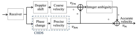
Figure 1.
The process of velocity measured by coherent Doppler sonar assisted by frequency shift (CHDSF).
The core algorithm in CHDSF is to calculate the integer ambiguity . As shown in Figure 1, the velocity measured by frequency shift without noise is equal to the velocity calculated by phase change without noise and the integer ambiguity, which can be expressed as below:
where
is the velocity measured by Doppler shift;
is the measurement error of ;
is the velocity measured by CHDS;
is the measurement error of .
According to Equation (8), the integer ambiguity can be obtained as:
where
If the value is larger than −0.5 and less than 0.5, can be calculated as
where the function is to obtain the nearest integer value.
2.3. Error Analysis
Due to the Gaussian white noise effect, the measurement errors and follow the Gaussian distribution [12], which are:
Then, the probability density function of error is
where
Suppose the calculation of the integer ambiguity contains an integer error (), it occurs when
According to Equations (14) and (16), the probability of occurring can be expressed as
Based on Equation (6), (13) and (17), the measurement error of velocity measured by CHDSF can be deduced, and the standard deviation () is
In Equation (18), the measurement error is affected by the measurement error and the integer ambiguity error . is small and difficult to be improved. The occurrence of directs impulsive noise, which influences significantly. To reduce the measurement error, the Kalman filter and linear prediction are introduced.
2.4. Kalman Filter and Linear Prediction
As shown in Equation (11), is estimated by , and Therefore, the value of depends on , and . is the denominator of Equation (10), which means that a large directs a small value of . A small value of will decrease the value of . However, is limited by “range-velocity” ambiguity. Although multiple time intervals [12,13] and carrier frequencies [14,15] were used to enlarge the value of , the maximum measurable speed is still limited. Compared with , is larger and contributes more in . In consequence, decreasing will reduce , and then improve the accuracy of measured velocity. Averaging is normally used to decreasing [4], but it generates a time delay for the system. To reduce without time delay, Kalman filter is introduced.
The Kalman filter was first developed in 1960 to solve the discrete data linear filtering problem [20]. It has been wildly used since, especially in the area of autonomous [21,22] or assisted navigation [23]. The Kalman filter can support estimations of past, present, and even future states, even when the precise nature of the modeled system is unknown.
The Kalman filter is constructed by time update equations and measurement update equations. The state of a discrete-time controlled process expressed by difference equation is shown as below:
where
is the input;
is the matrix relating the state at time step to +1;
is the matrix relating the control input to the state ;
is the process noise, following normal probability distribution:
Then, the equations for the time update are presented below:
where
is a priori state estimate;
is a posteriori state estimate;
is a priori estimate error covariance;
is a posteriori estimate error covariance.
The measurement can be expressed as:
where
is the matrix relating the state to the measurement ;
is the process noise, following normal probability distribution:
The equations for the measurement update are presented below:
where is the gain or blending factor that minimizes the posteriori error covariance.
After calculating time and measurement updates at some time, the process will repeat with the previous and posteriori estimates to predict the new a priori estimates. This recursive nature of the Kalman filter provides the benefit to decrease the measurement error during measurement without time delay.
Although the Kalman filter can deduce the measurement error of velocity calculated by frequency shift, it cannot clear the error generated by wrong estimation of . When the integer ambiguity error is non-zero, impulsive noise will appear. Hence, linear prediction [24] is introduced to deduce the impulsive noise. The prediction velocity of the th measured velocity () can be expressed as
where is the number of taps and is the prediction coefficient.
The difference between the predict velocity and measured velocity is defined as , which is
If the impulsive noise exists, can be estimated as
Based on the estimated , the measured velocity of CHDSF using the Kalman filter and linear prediction is
The flow chart of the whole data processing in CHDSF using the Kalman filter and linear prediction is shown in Figure 2.
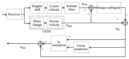
Figure 2.
Data processing of CHDSF using the Kalman filter and linear prediction.
3. Experiments
The structure of the experiment system is shown in Figure 3. A square pulse is generated by the waveform generator. Then, the generated pulse is amplified by an amplifier and transmitted by a projector in a water tank. The transmitted signal is received by a hydrophone and the received signal is amplified by another amplifier. Both the transmitted and received signals are sampled by an acquisition card. In the experiment, the hydrophone is moved towards projector forward and backward by a 3D moving device. The equipment used in our system are shown in Table 1. The experiment system is shown in Figure 4. The parameters used in the experiments are shown in Table 2.
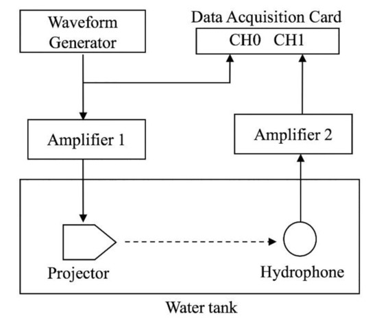
Figure 3.
Structure of experiment system.

Table 1.
Equipment information.
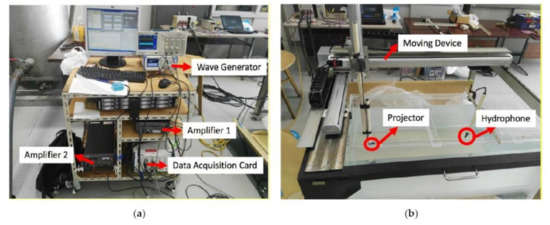
Figure 4.
Experiment system: (a) signal generator and receiver, including wave generator, two amplifiers and data acquisition card; (b) moving system, including moving device, projector and hydrophone.
Table 2.
Equipment parameters.
4. Results and Discussion
Based on the parameters in the experiment, the maximum velocity of CHDS is 0.181 m/s, which is less than the moving velocity. Therefore, CHDS cannot provide correct measurement results. The measured velocity by CHDS, frequency shift and CHDSF under the SNR of 2.5 dB is shown in Figure 5. Figure 5a is the velocity measured by CHDS, which is precise, but contains velocity drift. Velocity measured by frequency shift in Figure 5b is around true value, but noisy. The measurement error of frequency shift directs impulsive noise in the velocity measurement of CHDSF, making the measured velocity unacceptable. The measured velocity by CHDSF is shown in Figure 5c, and the comparison of the three methods is shown in Figure 5d.
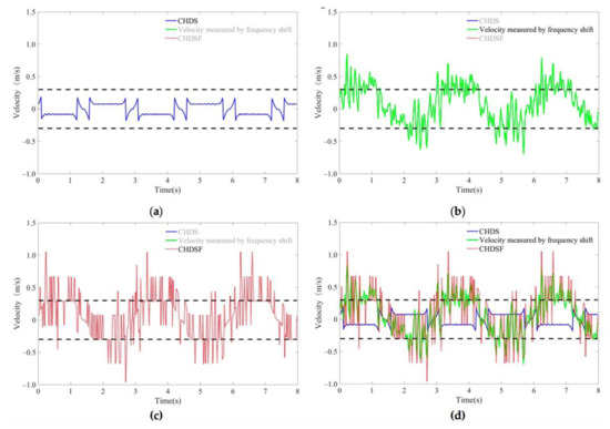
Figure 5.
Measured speed of 0.300 m/s (black dash line) by CHDS, frequency shift and CHDSF: (a) velocity measured by CHDS; (b) velocity measured by frequency shift; (c) velocity measured by CHDSF; (d) comparison of velocities measured by 3 methods.
The impulsive noise in CHDSF seriously disturbs the velocity measurement. Therefore, the Kalman filter and linear prediction are introduced; the measured velocity is shown in Figure 6. The parameters used in the Kalman filter and linear prediction are shown in Table 3. The velocity measured by CHDSF using the Kalman filter and linear prediction is accurate and precise. Impulsive noise is reduced significantly.
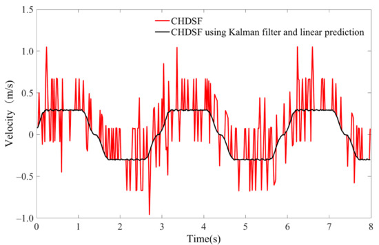
Figure 6.
Velocity measured by CHDSF using the Kalman filter and linear prediction.
Table 3.
Parameters used in the Kalman filter and linear prediction.
A median filter is adopted to erase impulsive noise [25]. The filtered results by median filter with 0.5 s are shown in Figure 7b. Generally, measured velocity by median filter performs well in the process of smooth moving, but it generates a significant bias when the moving velocity is changing. A mean filter is normally used in sonar systems to improve the accuracy of the measured velocity. With 0.5 s averaging, the measured velocity by CHDSF is shown in Figure 7c. The averaged velocity of CHDSF erases the impulsive noise, but it loses detail moving information and the accuracy is worse than the other two filters. The comparison of the three filters is shown in Figure 7d.
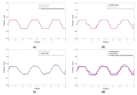
Figure 7.
Velocity measured by CHDSF using the Kalman filter and linear prediction, median filter and mean filter: (a) velocity measured by CHDSF using the Kalman filter and linear prediction; (b) velocity measured by CHDSF using median filter; (c) velocity measured by CHDSF using mean filter; (d) comparison of velocities measured by CHDSF using 3 filters.
The velocities measured by CHDSF with the 3 filters at the SNR of −3.6 dB and 7.7 dB are shown in Figure 8. CHDSF using the Kalman filter and linear prediction can provide accurate and precise velocity both in Figure 8a,b. CHDSF using the median filter cannot clear the impulsive noise in low SNR as shown in Figure 8a. Mean filter can reduce impulsive noise, but it has a larger bias compared with the other two filters. Both median and mean filters generate time delay, while the method using the Kalman filter and linear prediction does not.
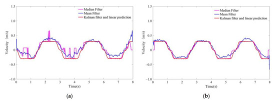
Figure 8.
Velocity measured by CHDSF using the Kalman filter and linear prediction method, median filter and mean filter in different SNRs: (a) SNR = −3.6 dB; (b) SNR = 7.7 dB.
The standard deviation (STD) of measured velocity by CHDSF and CHDSF using three filters is shown in Figure 9. The detail data are shown in Table 4. The process of movement includes acceleration, deceleration and uniform velocity. The STD is calculated in the process that the hydrophone moves with a uniform velocity. As shown in Figure 9, the STD of CHDSF using filters decrease the measurement error significantly. In high SNR (>3 dB), the Kalman filter and linear prediction method can provide velocity measurement with small error, which is better than the mean filter. In low SNR (<−3 dB), the Kalman filter and linear prediction method still can measure the velocity accurately and precisely, but the measurement errors of median and mean filters are large. Thus, CHDSF using the Kalman filter and linear prediction can provide small measurement error in a large range of SNR.
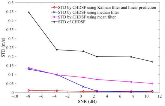
Figure 9.
Standard deviation of velocity measured by CHDSF and CHDSF using 3 filters.
Table 4.
Standard deviation of measured velocity by CHDSF and CHDSF using 3 filters.
5. Conclusions
CHDSF is proposed to take both advantages of CHDS and velocity measured by frequency shift, namely, measuring velocity without velocity ambiguity. However, the wrong estimation of the integer ambiguity generates impulsive noise. Therefore, the Kalman filter and linear prediction are introduced in CHDSF to remove the impulsive noise. First, the Kalman filter is used in the velocity measured by frequency shift to decrease the measurement error. Then the difference between the predicted velocity by linear prediction and the measured velocity by CHDSF is used to remove the impulsive noise. Experiments were carried out to evaluate the performance of CHDSF using the Kalman filter and linear prediction. A comparison of CHDSF using the Kalman filter and linear prediction method, median filter and mean filter was presented. The experiment and comparison results showed that CHDSF using the Kalman filter and linear prediction can provide accurate and precise velocity without velocity ambiguity. Compared with CHDSF using median and mean filter, the velocity measured by the proposed method had small standard deviation and a short time lag in a large range of SNR. Consequently, coherent Doppler sonar assisted by frequency shift, Kalman filter and linear prediction can provide accurate and precise velocity with short time lag, which could bring benefits for docking, navigation and oceanic engineering.
Author Contributions
Conceptualization, methodology, P.L. and N.K.; formal analysis, P.L.; writing and funding acquisition, Y.L. All authors have read and agreed to the published version of the manuscript.
Funding
This research was funded by Fundamental Research Funds for the Central Universities, grant number 3132020136, and National Key Research and Development Program of China, grant number 2018YFC0810403.
Institutional Review Board Statement
The study does not involve humans or animals.
Informed Consent Statement
The study does not involve humans.
Data Availability Statement
The data presented in this study are available on request from the corresponding author. The data are not publicly available due to the laboratory regulations.
Conflicts of Interest
The authors declare no conflict of interest.
References
- Tatsumi, K.; Kubota, T.; Fujii, H.; Kouguchi, N.; Arai, Y. Ship’s Speed Information Standards in Docking/Leaving Maneuvering Based on Questionnaire Survey. J. Jpn. Inst. Navig. 2008, 118, 31–37. [Google Scholar] [CrossRef]
- Yokogawa Denshikiki Co. Ltd. General Specification of EML500. Available online: https://static.mackaycomm.com/wp-content/uploads/2016/12/Yokogawa_EML500_SpeedLog_spec_2002_Mackay.pdf (accessed on 20 December 2020).
- Tatsumi, K.; Fujii, H.; Kubota, T.; Okuda, S.; Arai, Y.; Kouguchi, N.; Yamada, K. Performance Requirement of Ship’s Speed in Docking/Anchoring Maneuvering. In Proceedings of the International Association Institute of Navigation IAIN 06, Jeju, Korea, 18–20 October 2006. [Google Scholar]
- Yoo, Y.; Nakama, Y.; Kouguchi, N.; Song, C. Experimental Result of Ship’s Maneuvering Test Using GPS. J. Navig. Port Res. 2009, 33, 99–104. [Google Scholar] [CrossRef]
- Arai, Y.; Hori, A.; Okuda, S.; Yamada, K. Strategic Application of Two Axes Velocities Information for Ship Maneuvering. In Proceedings of the IAIN Congress, Stockholm, Sweden, 27–30 October 2009. [Google Scholar]
- Aray, Y.; Pedersen, E.; Kouguchi, N.; Yamada, K. The Availability of VI-GPS for Ship-Operation. In Proceedings of the ANC 2010, Inchon, Korea, 4–6 November 2010. [Google Scholar]
- Beiter, S.; Poquette, R.; Filipo, B.S.; Goetz, W. Precision Hybrid Navigation System for Varied Marine Applications. In Proceedings of the IEEE 1998 Position Location and Navigation Symposium, Palm Springs, CA, USA, 20–23 April 1996. [Google Scholar]
- Lohrmann, A.; Hackett, B.; Roed, L.P. High resolution measurements of turbulence, velocity and stress using a pulse-to-pulse coherent sonar. J. Atmos. Ocean Tech. 1990, 7, 19–37. [Google Scholar] [CrossRef]
- Veron, F.; Melville, W.K. Pulse-to-pulse coherent Doppler measurements of waves and turbulence. J. Atmos. Ocean Tech. 1999, 16, 1580–1597. [Google Scholar] [CrossRef]
- Lhermitte, R. and Serafin, R. Pulse-to-pulse coherent Doppler sonar signal processing techniques. J. Atmos. Ocean Tech. 1984, 1, 293–308. [Google Scholar] [CrossRef]
- Zedel, L. Modeling pulse-to-pulse coherent Doppler sonar. J. Atmos. Ocean Tech. 2008, 25, 1834–1844. [Google Scholar] [CrossRef]
- Holleman, I.; Beekhuis, H. Analysis and correction of dual PRF velocity data. J. Atmos. Ocean Tech. 2003, 20, 443–453. [Google Scholar] [CrossRef]
- Joe, P.; May, P.T. Correction of dual PRF velocity errors for operational Doppler weather radars. J. Atmos. Ocean Tech. 2003, 20, 429–442. [Google Scholar] [CrossRef]
- Hay, A.E.; Zedel, L.; Craig, R.; Paul, W. Multi-frequency, Pulse-to-pulse Coherent Doppler Sonar Profiler. In Proceedings of the 9th IEEE/OES/CMTC Working Conference on Current Measurement Technology, Charleston, SC, USA, 17–19 March 2008. [Google Scholar]
- Zedel, L.; Hay, A.E. Resolving velocity ambiguity in multifrequency, pulse-to-pulse coherent Doppler sonar. IEEE J. Ocean. Eng. 2010, 35, 847–851. [Google Scholar] [CrossRef]
- Liu, P.; Kouguchi, N. Combined Method of Conventional and Coherent Doppler Sonar to Avoid Velocity Ambiguity. J. Mar. Acoust. Soc. Jpn. 2014, 41, 103–112. [Google Scholar] [CrossRef]
- Liu, P.; Kouguchi, N. Measurement Error Analysis of Combined Doppler Sonar Using Adaptive Algorithm. J. Mar. Acoust. Soc. Jpn. 2015, 42, 11–22. [Google Scholar] [CrossRef]
- Dillon, J.; Zedel, L.; Hay A., E. On the Distribution of Velocity Measurements From Pulse-to-Pulse Coherent Doppler Sonar. IEEE J. Ocean. Eng. 2012, 37, 613–625. [Google Scholar] [CrossRef]
- Burdic, W.S. Radar Signal Analysis; Prentice-Hall. Inc.: Upper Saddle River, NJ, USA, 1968; Chapter 5. [Google Scholar]
- Kalman, R.E. A New Approach to Linear Filtering and Prediction Problems. Trans. ASME J. Basic Eng. 1960, 82, 35–45. [Google Scholar] [CrossRef]
- Shi, Y.; Fang, H.; Yan, M. Kalman filter-based adaptive control for networked systems with unknown parameters and randomly missing outputs. Int. J. Robust Nonlin. 2010, 19, 1976–1992. [Google Scholar] [CrossRef]
- Thomas, S.; Hofmann, W.; Werner, R. Improving operational performance of active magnetic bearings using Kalman filter and state feedback control. IEEE T. Ind. Electron. 2011, 59, 821–829. [Google Scholar]
- Lefferts, E.J.; Markley, F.L.; Shuster, M.D. Kalman filtering for spacecraft attitude estimation. J. Guid. Control Dynam. 1982, 5, 417–429. [Google Scholar]
- Arata, K.; Kensaku, F.; Yoshio, I.; Yutaka, F. A noise reduction method based on linear prediction analysis. Electr. Commun. Jpn. 2003, 86. [Google Scholar]
- Ravi Kishore, T.; Deergha Rao, K. Efficient median filter for restoration of image and video sequences corrupted by impulsive noise. IETE J. Res. 2010, 56, 219–226. [Google Scholar] [CrossRef]
Publisher’s Note: MDPI stays neutral with regard to jurisdictional claims in published maps and institutional affiliations. |
© 2021 by the authors. Licensee MDPI, Basel, Switzerland. This article is an open access article distributed under the terms and conditions of the Creative Commons Attribution (CC BY) license (http://creativecommons.org/licenses/by/4.0/).