
Modeling the Habitat Distribution of Acanthopagrus schlegelii in the Coastal Waters of the Eastern Taiwan Strait Using MAXENT with Fishery and Remote Sensing Data


 , ,
, ,  , ,
, ,
Abstract
:1. Introduction
2. Materials and Methods
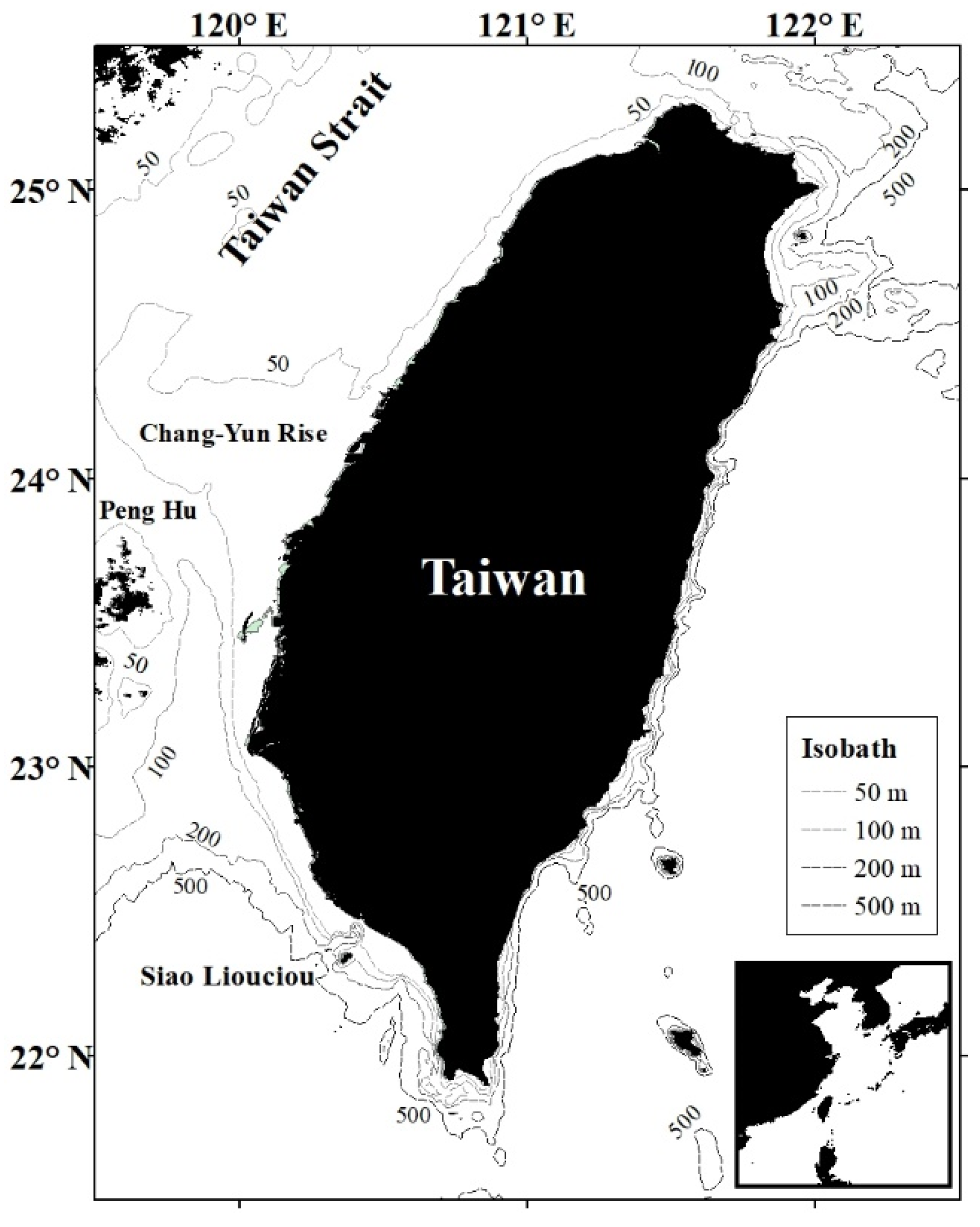
2.1. Study Area
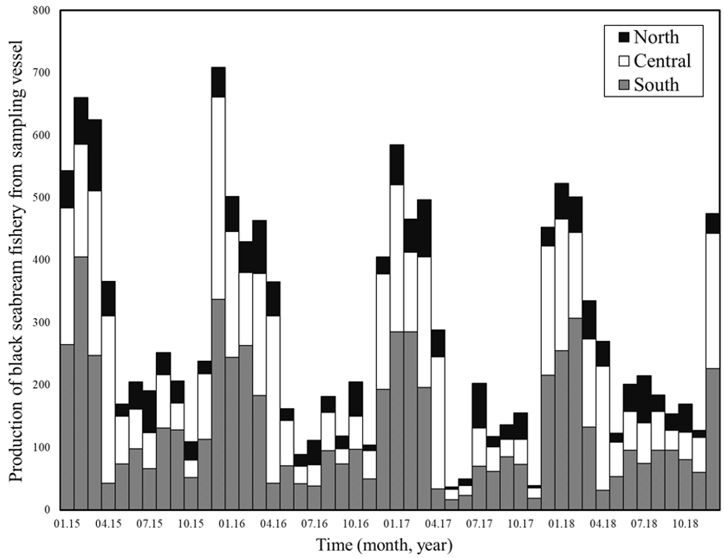
2.2. Fishery Data
2.3. Environmental Parameters
2.4. Development and Evaluation of Habitat Model
2.5. Spatial Mapping and Validation
3. Results
3.1. Seasonal and Environmental Effects
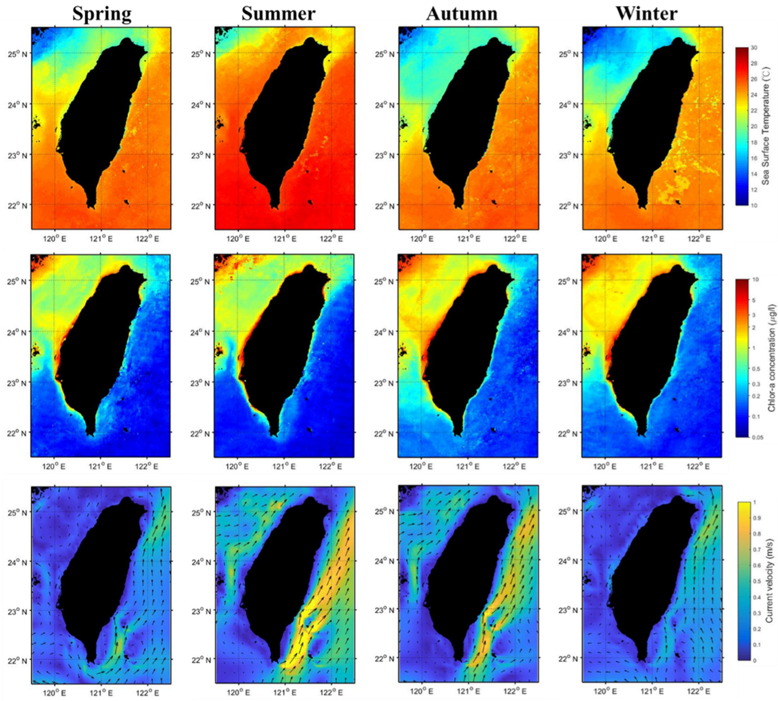
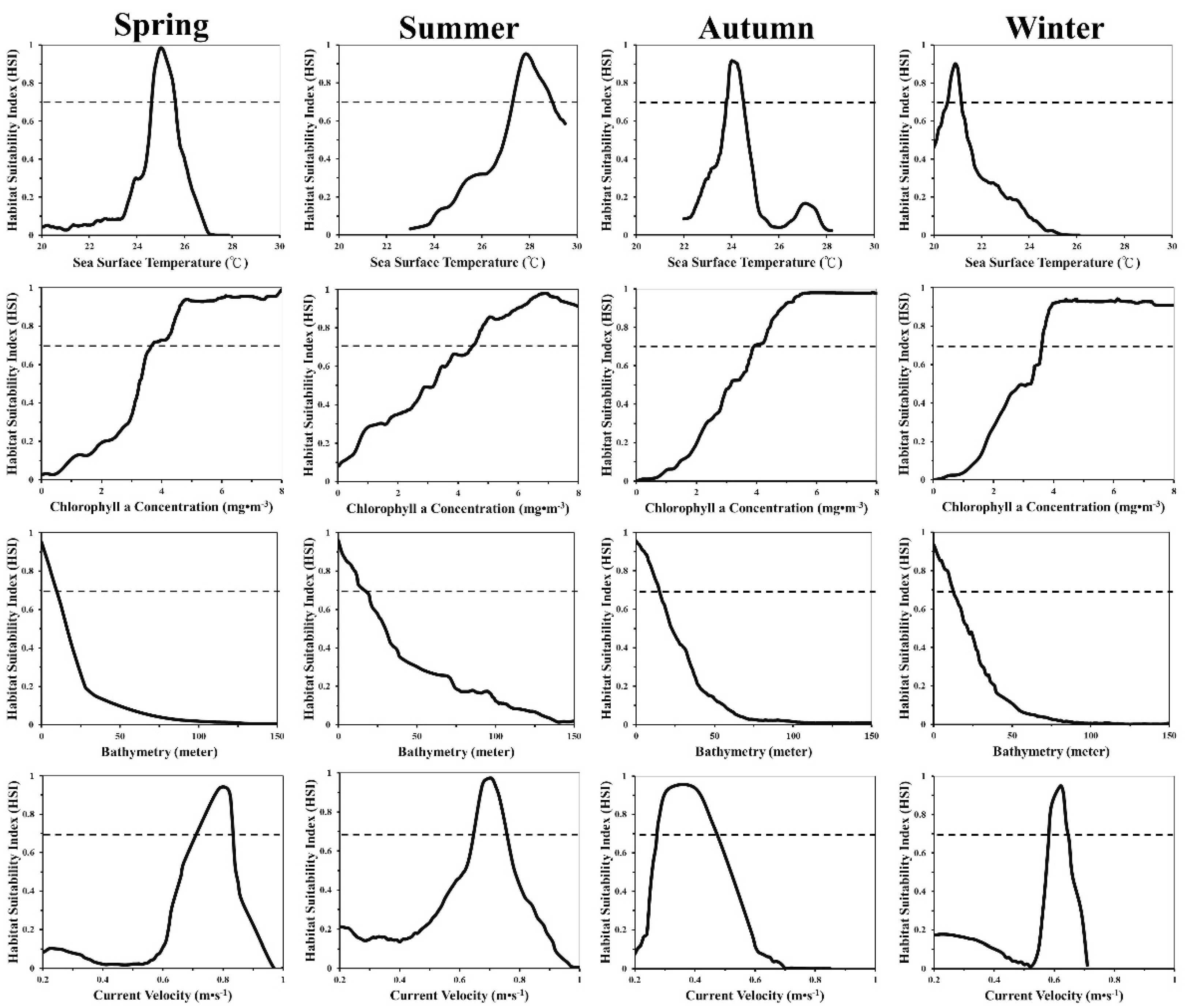
3.2. Environmental Conditions in Black Sea Bream Habitats
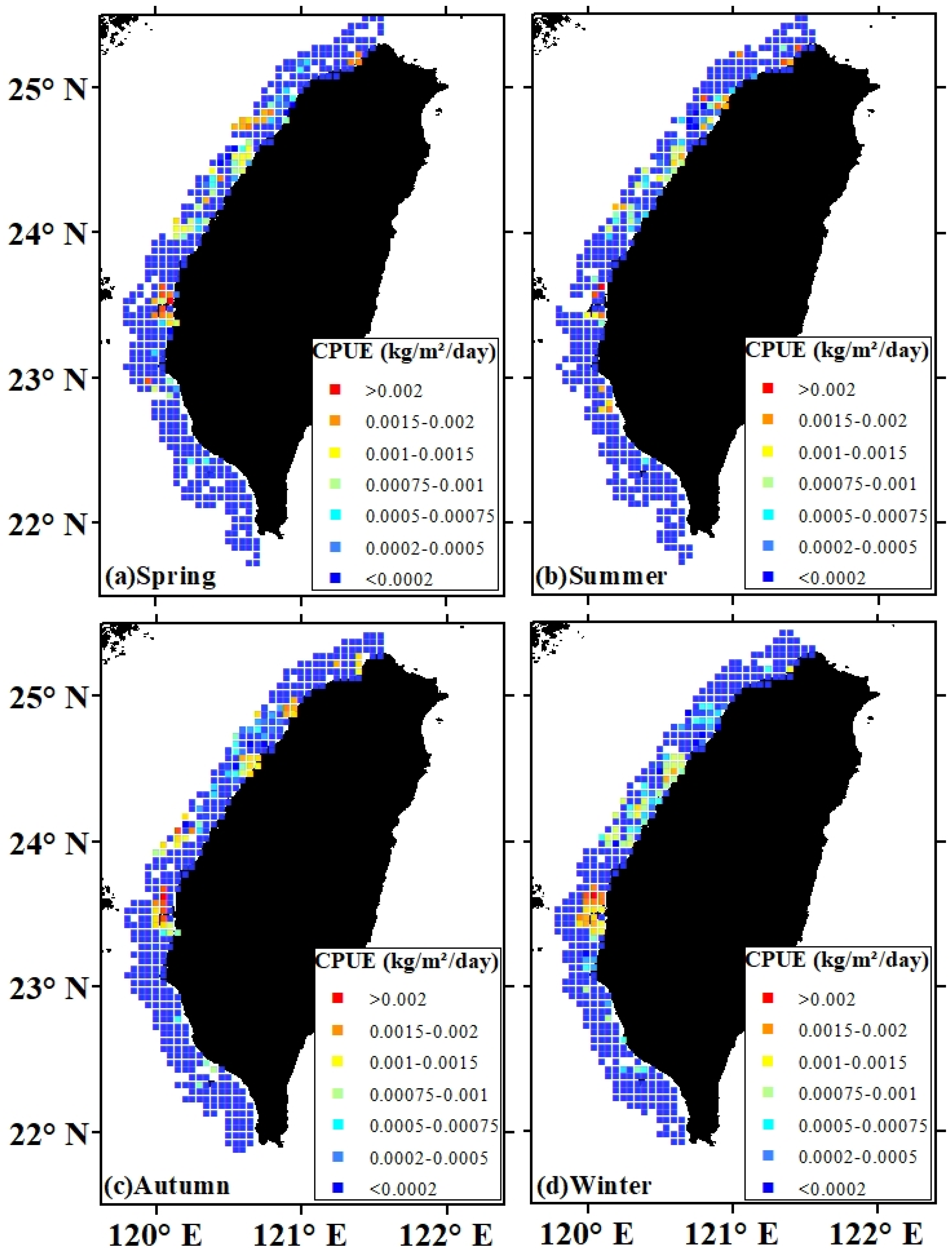
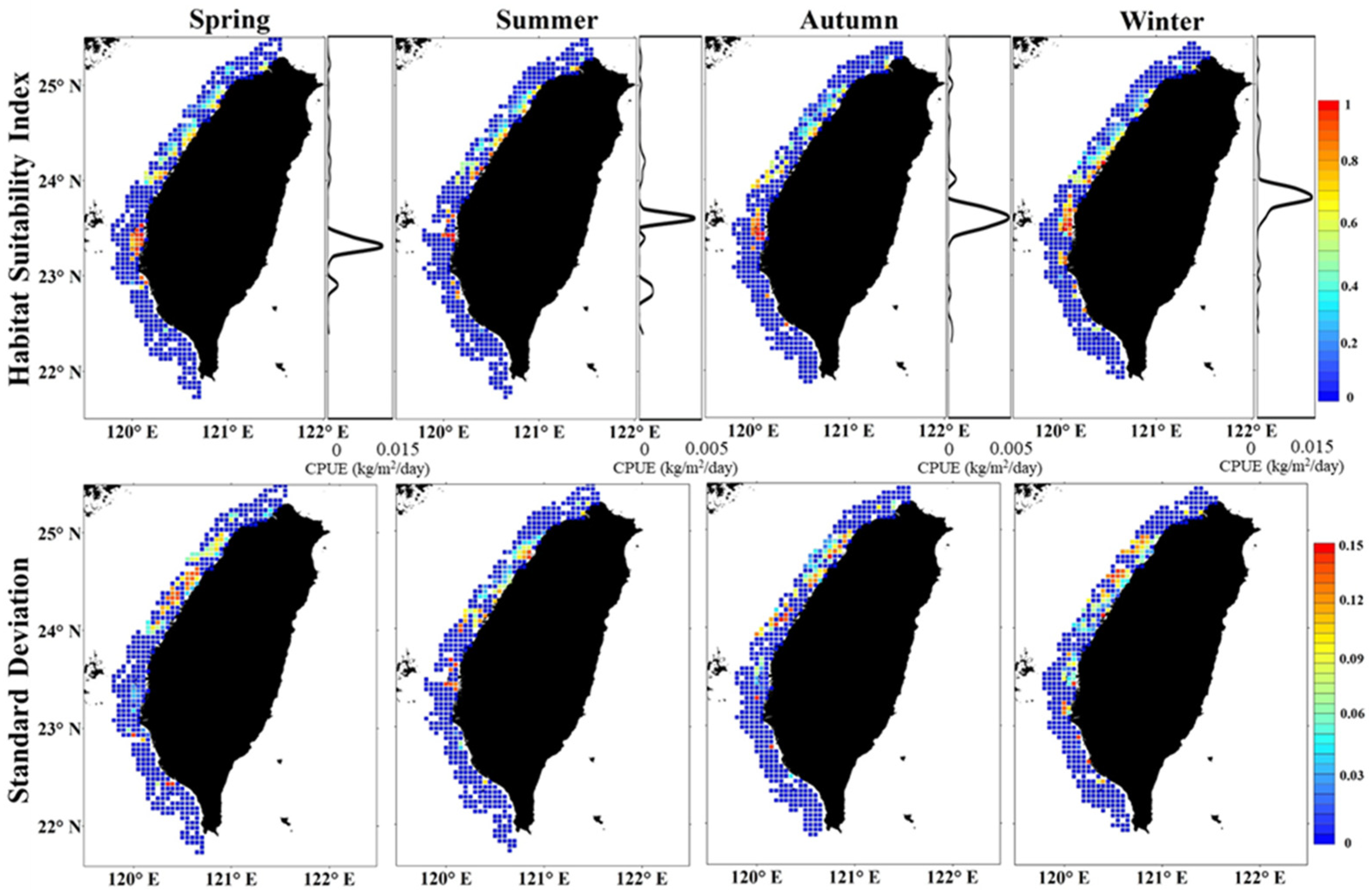
3.3. Spatial Patterns of Habitat and Uncertainty
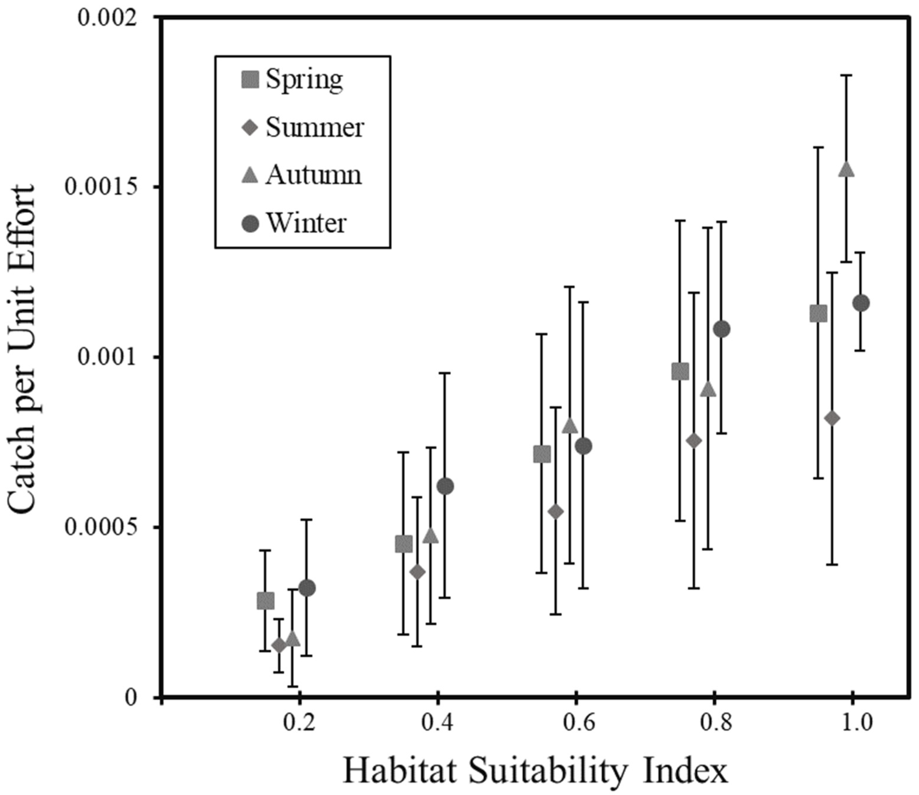
3.4. Validation of Habitat Model
4. Discussion
4.1. Modeling the Habitat Distribution
4.2. Environmental Impacts on Habitat
4.3. Spatial Aggregation and Seasonal Shift
5. Conclusions
Author Contributions
Funding
Institutional Review Board Statement
Informed Consent Statement
Data Availability Statement
Acknowledgments
Conflicts of Interest
References
- Food and Agriculture Organization. The State of World Fisheries and Aquaculture: Opportunities and challenges. Food Agric. Organ. United Nations Rome 2014, 4, 40–41. [Google Scholar]
- Food and Agriculture Organization. The State of World Fisheries and Aquaculture 2006; Food and Agriculture Organization of the United Nations: Rome, Italy, 2007; p. 162. Available online: https://www.fao.org/3/a0699e/A0699E.pdf (accessed on 10 December 2021).
- Root, T.L.; Price, J.T.; Hall, K.R.; Schneider, S.H.; Rosenzweigk, C.; Pounds, J.A. Fingerprints of global warming on wild animals and plants. Nature 2003, 421, 57–60. [Google Scholar] [CrossRef]
- Beaugrand, G. Monitoring pelagic ecosystems using plankton indicators. ICES J. Mar. Sci. 2005, 62, 333–338. [Google Scholar] [CrossRef] [Green Version]
- King, J.R. Report of the study group on fisheries and ecosystem responses to recent regime shifts. North Pac. Mar. Sci. Organ. Sci. Rep. 2005, 28, 168. [Google Scholar]
- Chou, L.Y. A Study on Time Series Analysis of the Landings from the Fishers, Associations in Western Taiwan. Master’s Thesis, Department of Environmental Biology and Fisheries Science, NTOU, Keelung, Taiwan, 2006. (In Chinese). [Google Scholar]
- Wang, T.K. Studies on the Management and Reformation of Taiwan Inshore Fishery. Master’s Thesis, Institute of Marine Affairs, National Sun Yat-Sen University, Kaohsiung, Taiwan, 2012; pp. 1–253. (In Chinese). [Google Scholar]
- Cheung, W.W.L.; Lam, V.W.Y.; Sarmiento, J.L.; Kearney, K.; Watson, R.E.G.; Zeller, D.; Pauly, D. Large-scale redistribution of maximum fisheries catch potential in the global ocean under climate change. Glob. Chang. Biol. 2010, 16, 24–35. [Google Scholar] [CrossRef]
- Allison, E.H.; Perry, A.L.; Badjeck, M.C.; Adger, W.N.; Brown, K.; Conway, D.; Halls, A.S.; Pilling, G.M.; Reynolds, J.D.; Andrew, N.L.; et al. Vulnerability of national economies to the impacts of climate change on fisheries. Fish Fish. 2009, 10, 173–196. [Google Scholar] [CrossRef] [Green Version]
- Joseph, V.; Thornton, A.; Pearson, S.; Paull, D. Occupational transitions in three coastal villages in Central Java, Indonesia, in the context of sea level rise: A case study. Nat. Hazards 2013, 69, 675–694. [Google Scholar] [CrossRef]
- Selig, E.R.; Turner, W.R.; Troeng, S.; Wallace, B.P.; Halpern, B.S.; Kaschner, K.; Lascelles, B.G.; Carpenter, K.E.; Mittermeier, R.A. Global priorities for marine biodiversity conservation. PLoS ONE 2014, 9, e82898. [Google Scholar] [CrossRef]
- Morato, T.; Hoyle, S.D.; Allain, V.; Nicol, S.J. Seamounts are hotspots of pelagic biodiversity in the open ocean. Proc. Natl. Acad. Sci. USA 2010, 107, 9707–9711. [Google Scholar] [CrossRef] [PubMed] [Green Version]
- Masuda, H.; Amaoka, K.; Araga, C.; Uyeno, T.; Yoshino, T.; Muzik, K. The Fishes of the Japanese Archipelago; Tokai University Press: Tokyo, Japan, 1984. [Google Scholar]
- Hong, W.S.; Zhang, Q.Y. Review of captive bred species and fry production of marine fish in China. Aquaculture 2003, 227, 305–318. [Google Scholar] [CrossRef]
- Shao, Q.J.; Ma, J.J.; Xu, Z.R.; Hu, W.L.; Xu, J.Z.; Xie, S.Q. Dietary phosphorus requirement of juvenile black sea bream, Sparus macrocephalus. Aquaculture 2008, 277, 92–100. [Google Scholar] [CrossRef]
- Gonzalez, E.B.; Nagasawa, K.; Umino, T. Stock enhancement program for black sea bream (Acanthopargrus schlegelii) in Hiroshima Bay: Monitoring the genetic effects. Aquaculture 2008, 276, 36–43. [Google Scholar] [CrossRef] [Green Version]
- Gonzalez, E.B.; Umino, T.; Nagasawa, K. Stock enhancement programme for black sea bream, Acanthopagrus schlegelii (Bleeker), in Hiroshima Bay, Japan: A review. Aquac. Res. 2008, 39, 1307–1315. [Google Scholar] [CrossRef]
- Gonzalez, E.B.; Murakami, T.; Yoneji, T.; Nagasawa, K.; Umino, T. Reduction in size-at-age of black sea bream (Acanthopagrus schlegelii) following intensive releases of cultured juveniles in Hiroshima Bay, Japan. Fish. Res. 2009, 99, 130–133. [Google Scholar] [CrossRef]
- Lu, J.H.; Lee, S.L. Observations of changes in the fish species composition in the coastal zone at the Kuroshio Current and China Coastal Current front during climate change using set-net tianfishery (1993–2011). Fish. Res. 2014, 155, 103–113. [Google Scholar] [CrossRef]
- Sinaga, S.; Chen, T.P.; Lu, H.J. Reproductive biology study of blackhead seabream (Acanthopagrus schlegelii) in Miaoli waters of Taiwan. J. Fish. Soc. Taiwan 2019, 46, 97–107. [Google Scholar]
- Chang, C.F.; Yueh, W.W. Annual cycle of gonadal histology and steroid profiles in the juvenile males and adult females of the protandrous black porgy, Acanthopagrus schlegelii. Aquaculture 1990, 91, 179–196. [Google Scholar] [CrossRef]
- Teal, L.R.; Marras, S.; Peck, M.A.; Domenici, P. Physiology-based modelling approaches to characterize fish habitat suitability: Their usefulness and limitations. Estuar. Coast. Shelf Sci. 2018, 201, 56–63. [Google Scholar] [CrossRef]
- Guisan, A.; Zimmermann, N.E. Predictive habitat distribution models in ecology. Ecol. Model. 2000, 135, 147–186. [Google Scholar] [CrossRef]
- Elith, J.; Leathwick, J.R. Species distribution models: Ecological explanation and prediction across space and time. Annu. Rev. Ecol. Evol. Syst. 2009, 40, 677–697. [Google Scholar] [CrossRef]
- Alabia, I.D.; Saitoh, S.I.; Mugo, R.; Igarashi, H.; Ishikawa, Y.; Usui, N.; Kamachi, M.; Awaji, T.; Seito, M. Seasonal potential fishing ground prediction of neon flying squid (Ommastrephes bartramii) in the western and central North Pacific. Fish. Oceanogr. 2015, 24, 190–203. [Google Scholar] [CrossRef]
- Franca, S.; Cabral, H.N. Predicting fish species distribution in estuaries: Influence of species’ ecology in model accuracy. Estuar. Coast. Shelf Sci. 2016, 180, 11–20. [Google Scholar] [CrossRef]
- Warren, D.L.; Seifert, S.N. Ecological niche modeling in Maxent: The importance of model complexity and the performance of model selection criteria. Ecol. Appl. 2011, 21, 335–342. [Google Scholar] [CrossRef] [Green Version]
- Phillips, S.J.; Anderson, R.P.; Schapire, R.E. Maximum entropy modelling of species geographic distributions. Ecol. Model. 2006, 190, 231–259. [Google Scholar] [CrossRef] [Green Version]
- Phillips, S.J.; Anderson, R.P.; Dudik, M.; Schapire, R.E.; Blair, M.E. Opening the black box: An open-source release of Maxent. Ecography 2017, 40, 887–893. [Google Scholar] [CrossRef]
- Lefkaditou, E.; Politou, C.Y.; Palialexis, A.; Dokos, J.; Cosmopoulos, P.; Valavanis, V.D. Influences of environmental variability on the population structure and distribution patterns of the short-fin squid Illes coindetii (Cephalopoda: Ommastrephidae) in the Eastern Ionian Sea. Hydrobiologia 2008, 612, 71–90. [Google Scholar] [CrossRef]
- Alabia, I.D.; Saitoh, S.I.; Mugo, R.; Igarashi, H.; Ishikawa, Y.; Usui, N.; Kamachi, M.; Awaji, T.; Seito, M. Identifying pelagic habitat hotspots of neon flying squid in the temperate waters of the central North Pacific. PLoS ONE 2015, 10, e0142885. [Google Scholar] [CrossRef] [Green Version]
- Fishery Agency. Fisheries Statistical Yearbook Taiwan Area; Taiwan Fisheries Administration, Executive Yuan: Kaohsiung City, Taiwan, 2017. (In Chinese) [Google Scholar]
- Lo, K.C.; Teng, S.Y.; Wang, Y.C.; Lee, M.A.; Lin, J.L.; Lu, T.H.; Huang, I.L. Resource structure of an artisanal gillnet fishery in the coastal water of Tamsui, Taiwan. J. Fish. Soc. Taiwan 2017, 44, 147–157. [Google Scholar]
- Su, N.J.; Lu, Y.S.; Cheng, C.Y.; Huang, L.C.; Li, C.H. Investigation on fishing activity and catch composition of coastal gillnet fisheries in waters off northwestern Taiwan. J. Fish. Soc. Taiwan 2017, 44, 159–169. [Google Scholar]
- Iwatsuki, Y.; Carpenter, K.E. Acanthopagrus taiwanensis, a new sparid fish (Perciformes), with comparisons to Acanthopagrus berda (Forsskal, 1775) and other nominal species of Acanthopagrus. Zootaxa 2006, 1201, 1–19. [Google Scholar] [CrossRef] [Green Version]
- Islam, M.S.; Tanaka, M. Impacts of pollution on coastal and marine ecosystems including coastal and marine fisheries and approach for management: A review and synthesis. Mar. Pollut. Bull. 2004, 48, 624–649. [Google Scholar] [CrossRef] [PubMed]
- Hsiao, P.Y.; Wu, Y.L.; Lan, K.W.; Lee, L.S. Seasonal variations of fishery resources structure of Trammel nets in the coastal water of Changyuen Rise, Taiwan. J. Fish. Soc. Taiwan 2017, 44, 171–183. [Google Scholar]
- Teng, S.Y.; Lee, M.A.; Hsu, J.; Lin, T.P.; Lin, Y.C.; Chang, Y. Assessing the vulnerability of fishery villages influenced by climate change and anthropogenic activity in the coastal zone of the Tamsui River. J. Mar. Sci. Technol. 2016, 24, 1115–1126. [Google Scholar]
- Kuo, Y.C.; Chan, J.W.; Wang, Y.C.; Shen, Y.L.; Chang, Y.; Lee, M.A. Long-term observation on sea surface temperature variability in the Taiwan Strait during the northeast monsoon season. Int. J. Remote Sens. 2018, 39, 4330–4342. [Google Scholar] [CrossRef]
- Hong, H.; Chai, F.; Zhang, C.; Huang, B.; Jiang, Y.; Hu, J. An overview of physical and biogeochemical processes and ecosystem dynamics in the Taiwan Strait. Cont. Shelf Res. 2011, 31, S3–S12. [Google Scholar] [CrossRef]
- Nip, T.H.; Ho, W.Y.; Kim Wong, C. Feeding ecology of larval and juvenile black seabream (Acanthopagrus schlegeli) and Japanese seaperch (Lateolabrax japonicus) in Tolo Harbour, Hong Kong. Environ. Biol. Fishes 2003, 66, 197–209. [Google Scholar] [CrossRef]
- Lee, M.A.; Yang, Y.C.; Shen, Y.L.; Chang, Y.; Tsai, W.S.; Lan, K.W.; Kuo, Y.C. Effects of an unusual cold-water intrusion in 2008 on the catch of coastal fishing methods around Penghu Islands, Taiwan. Terr. Atmos. Ocean. Sci. 2014, 25, 107–120. [Google Scholar] [CrossRef] [Green Version]
- Liu, K.K.; Tang, T.Y.; Gong, G.C.; Chen, L.Y.; Shiah, F.K. Cross-shelf and along–shelf nutrient fluxes derived from flow fields and chemical hydrography observed in the southern East China Sea off northern Taiwan. Cont. Shelf Res. 2000, 20, 493–523. [Google Scholar] [CrossRef]
- Maunder, M.N.; Punt, A.E. Standardizing catch and effort data: A review of recent approaches. Fish. Res. 2004, 70, 141–159. [Google Scholar] [CrossRef]
- Lee, M.A.; Chang, Y.; Sakaida, F.; Kawamura, H.; Cheng, C.H.; Chan, J.W.; Huang, I. Terr. Atmos. Ocean. Sci. 2005, 16, 1189–1204. [CrossRef] [Green Version]
- McClain, E.P.; Pichel, W.G.; Walton, C.C. Comparative performance of AVHRR-based multichannel sea surface temperatures. J. Geophys. Res. 1985, 90, 587–601. [Google Scholar] [CrossRef]
- NASA’s OceanColor Web. Available online: http://oceancolor.gsfc.nasa.gov/ (accessed on 10 December 2021).
- Bleck, R. An oceanic general circulation model framed in hybrid isopycnic-Cartesian coordinates. Ocean. Model. 2002, 4, 55–88. [Google Scholar] [CrossRef]
- Andrade, H.A. The relationship between the skipjack tuna (Katsuwonus pelamis) fishery and seasonal temperature variability in the southwestern Atlantic. Fish. Oceanogr. 2003, 12, 10–18. [Google Scholar] [CrossRef]
- Zainuddin, M.; Kiyofugi, H.; Saitoh, K.; Saitoh, S. Using multi-sensor satellite remote sensing and catch data to detect ocean hot spots for albacore (Thunnus alalunga) in the northwestern North Pacific. Deep-Sea Res. Part II 2006, 53, 419–431. [Google Scholar] [CrossRef]
- Chen, X.J.; Tian, S.Q.; Chen, Y.; Liu, B. A modeling approach to identify optimal habitat and suitable fishing grounds for neon flying squid (Ommastrephes bartramii) in the Northwest Pacific Ocean. Fish. Bull. 2010, 108, 1–14. [Google Scholar]
- Haig, J.A.; Lambert, G.I.; Sumpton, W.D.; Mayer, D.G.; Werry, J.M. Habitat features influence catch rates of near-shore bull shark (Carcharhinus leucas) in the Queensland Shark Control Program, Australia 1996-2012. Estuar. Coast. Shelf Sci. 2018, 200, 289–300. [Google Scholar] [CrossRef]
- Rupprecht, F.; Oldeland, J.; Finckh, M. Modelling potential distribution of the threatened tree species Juniperus oxycedrus: How to evaluate the predictions of different modelling approaches? J. Veg. Sci. 2011, 22, 647–659. [Google Scholar] [CrossRef]
- Jones, M.C.; Dye, S.R.; Pinnegar, J.K.; Warren, R.; Cheung, W.W.L. Modelling commercial fish distributions: Prediction and assessment using different approaches. Ecol. Model. 2012, 225, 133–145. [Google Scholar] [CrossRef]
- McClellan, C.M.; Brereton, T.; Dell’Amico, F.; Johns, D.G.; Cucknell, A.C.; Patrick, S.C.; Penrose, R.; Ridoux, V.; Solandt, J.L.; Stephan, E.; et al. Understanding the Distribution of Marine Megafauna in the English Channel Region: Identifying Key Habitats for Conservation within the Busiest Seaway on Earth. PLoS ONE 2014, 9, e89720. [Google Scholar]
- Swets, J.A. Measuring the accuracy of diagnostic systems. Science 1988, 240, 1285–1293. [Google Scholar] [CrossRef] [Green Version]
- Alabia, I.D.; Dehara, M.; Saitoh, S.I.; Hirawake, T. Seasonal habitat patterns of Japanese Common Squid (Todarodes Pacificus) inferred from satellite-based species distribution models. Remote Sens. 2016, 8, 921. [Google Scholar] [CrossRef] [Green Version]
- Dell, J.; Wilcox, C.; Hobday, A.J. Estimation of yellowfin tuna (Thunnus albacares) habitat in waters adjacent to Australia’s east coast: Making the most of commercial catch data. Fish. Oceanogr. 2011, 20, 383–396. [Google Scholar] [CrossRef]
- Jan, S.; Wang, J.; Chern, C.S.; Chao, S.Y. Seasonal variation of the circulation in the Taiwan Strait. J. Mar. Syst. 2002, 35, 249–268. [Google Scholar] [CrossRef]
- Wang, J.; Chern, C.S. On the distribution of bottom cold waters in Taiwan Strait during summertime. Acta Oceanogr. Taiwanica 1992, 25, 55–64. [Google Scholar]
- Belkin, I.M.; Lee, M.A. Long-term variability of sea surface temperature in Taiwan Strait. Clim. Chang. 2014, 124, 821–834. [Google Scholar] [CrossRef] [Green Version]
- Lin, S.F.; Tang, T.Y.; Jan, S.; Chen, C.J. Taiwan strait current in winter. Cont. Shelf Res. 2005, 25, 1023–1042. [Google Scholar] [CrossRef]
- Tian, S.Q.; Chen, X.J.; Chen, Y.; Xu, L.X.; Dai, X.J. Evaluating habitat suitability indices derived from CPUE and fishing effort data for Ommastrephes bartramii in the northwestern Pacific Ocean. Fish. Res. 2009, 95, 181–188. [Google Scholar] [CrossRef]
- Sedberry, G.R.; Loefer, J.K. Satellite telemetry tracking of swordfish, Xiphias gladius, off the eastern United States. Mar. Biol. 2001, 139, 355–360. [Google Scholar]
- Seki, M.P.; Polovina, J.J.; Kobayashi, D.R.; Bidigare, R.R.; Mitchum, G.T. An oceanographic characterization of swordfish (Xiphias gladius) longline fishing grounds in the springtime subtropical north Pacific. Fish. Oceanogr. 2002, 11, 251–266. [Google Scholar] [CrossRef]
- Fritsches, K.A.; Brill, R.W.; Warrant, E.J. Warm eyes provide superior vision in swordfishes. Curr. Biol. 2005, 15, 55–58. [Google Scholar] [CrossRef] [Green Version]
- Huang, J.F.; Lee, J.M. Production economics and profitability analysis of horizontal rack culture and horizontal rack culture coupled with raft-string culture methods: A case study of Pacific oyster (Crassostrea gigas) farming in Chiayi and Yunlin Counties, Taiwan. Aquac. Int. 2014, 22, 1131–1147. [Google Scholar] [CrossRef]
- Saito, H.; Nakanishi, Y.; Shigeta, T.; Umino, T.; Kawai, K.; Imabayashi, H. Effect of predation of fishes on oyster spats in Hiroshima Bay. Nippon. Suisan Gakkaishi 2008, 74, 809–815. (In Japanese) [Google Scholar] [CrossRef] [Green Version]
- Yamashita, H.; Katayama, S.; Komiya, T. Age and growth of black sea bream Acanthopagrus schlegelii (Bleeker 1854) in Tokyo Bay. Asian Fish. Sci. J. 2015, 28, 47–59. [Google Scholar] [CrossRef]
- Daskalov, G. Relating fish recruitment to stock biomass and physical environment in the Black Sea using generalized additive models. Fish. Res. 1999, 41, 1–23. [Google Scholar] [CrossRef]
- Sadovy, Y.; Cornish, A.S. Reef Fishes of Hong Kong; Hong Kong University Press: Hong Kong, China, 2000; p. 321. [Google Scholar]
- Zhang, R.Z. Fish Eggs and Larvae in the Coastal Waters of China; Shanghai Science and Technology Press: Shanghai, China, 1985. [Google Scholar]
- Nakabo, T. Fishes of Japan with Pictorial Keys to the Species, English Edition I; Tokai University Press: Tokai, Japan, 2002; p. 886. [Google Scholar]


| Environmental Variables | Sampling Interval | Spatial Resolution | Primary Source |
|---|---|---|---|
| Sea surface temperature (°C) | Daily | 0.01° | AVHRR |
| Chlorophyll-a concentration (mg/m3) | Daily | 0.01° | MODIS |
| Current velocity (m/s) | Daily | 1/12° | HYCOM |
| Bathymetry (m) | - | 1/60° | ETOPO1 |
| Environmental | Percent | Contribution | ||
|---|---|---|---|---|
| Variables | Spring | Summer | Autumn | Winter |
| Chl-a | 59.1 | 64.6 | 71.3 | 80.3 |
| Bathymetry | 21 | 22.7 | 20.1 | 12.6 |
| Current Velocity | 0.3 | 1.6 | 1 | 2.2 |
| SST | 19.6 | 11.1 | 7.6 | 5.9 |
| Test AUC | 0.949 | 0.955 | 0.959 | 0.967 |
| Training AUC | 0.973 | 0.978 | 0.966 | 0.979 |
Publisher’s Note: MDPI stays neutral with regard to jurisdictional claims in published maps and institutional affiliations. |
© 2021 by the authors. Licensee MDPI, Basel, Switzerland. This article is an open access article distributed under the terms and conditions of the Creative Commons Attribution (CC BY) license (https://creativecommons.org/licenses/by/4.0/).
Share and Cite
Teng, S.-Y.; Su, N.-J.; Lee, M.-A.; Lan, K.-W.; Chang, Y.; Weng, J.-S.; Wang, Y.-C.; Sihombing, R.I.; Vayghan, A.H. Modeling the Habitat Distribution of Acanthopagrus schlegelii in the Coastal Waters of the Eastern Taiwan Strait Using MAXENT with Fishery and Remote Sensing Data. J. Mar. Sci. Eng. 2021, 9, 1442. https://doi.org/10.3390/jmse9121442
Teng S-Y, Su N-J, Lee M-A, Lan K-W, Chang Y, Weng J-S, Wang Y-C, Sihombing RI, Vayghan AH. Modeling the Habitat Distribution of Acanthopagrus schlegelii in the Coastal Waters of the Eastern Taiwan Strait Using MAXENT with Fishery and Remote Sensing Data. Journal of Marine Science and Engineering. 2021; 9(12):1442. https://doi.org/10.3390/jmse9121442
Chicago/Turabian StyleTeng, Sheng-Yuan, Nan-Jay Su, Ming-An Lee, Kuo-Wei Lan, Yi Chang, Jinn-Shing Weng, Yi-Chen Wang, Riah Irawati Sihombing, and Ali Haghi Vayghan. 2021. "Modeling the Habitat Distribution of Acanthopagrus schlegelii in the Coastal Waters of the Eastern Taiwan Strait Using MAXENT with Fishery and Remote Sensing Data" Journal of Marine Science and Engineering 9, no. 12: 1442. https://doi.org/10.3390/jmse9121442
APA StyleTeng, S.-Y., Su, N.-J., Lee, M.-A., Lan, K.-W., Chang, Y., Weng, J.-S., Wang, Y.-C., Sihombing, R. I., & Vayghan, A. H. (2021). Modeling the Habitat Distribution of Acanthopagrus schlegelii in the Coastal Waters of the Eastern Taiwan Strait Using MAXENT with Fishery and Remote Sensing Data. Journal of Marine Science and Engineering, 9(12), 1442. https://doi.org/10.3390/jmse9121442