Analysis of Thermal Plume Dispersion into the Sea by Remote Sensing and Numerical Modeling

Abstract

The aim of this work was to study, by remote sensing and numerical modeling, the thermal dispersion of a plume discharged into the sea by a nuclear power plant. The case study is the thermal discharge of the Laguna Verde nuclear power plant, located on the coast of the Gulf of Mexico. First, the thermal plume dispersion was characterized by applying remote sensing for different scenarios. Afterwards, Delft3D-FLOW numerical simulations were performed to expand the analysis of the thermal processes for a case in which the thermal plume tends towards the intake of the power plant. This thermal analysis was carried out by comparing the behavior of different dimensionless parameters. Moreover, the results of the numerical simulations were used to investigate the performance of the AEM and the k-L and k-ε turbulence models, available in the Delft3D-FLOW model. An LES turbulence model contribution was also analyzed. The results show that forced convection is predominant near the plume discharge area and at the vicinity of the intake structure. According to the metrics calculated, all turbulence models produced good agreement with the remote sensing data, except when the LES scheme was considered. Finally, the use of remote sensing and numerical simulations is helpful to better understand thermal plume dispersion.

1. Introduction

Coastal zones are preferred locations for the operation of power plants due to the vast availability of seawater, which is used for cooling purposes. The water supply required by a nuclear power plant is higher than any other power source for a similar output by a factor of between 30% and 100% [1]. When the cooling cycle is complete, water is returned to the sea at an increased temperature. Consequently, thermal pollution is generated by thermal plumes that are mixed into the sea.

From an environmental point of view, thermal plumes are the cause of destruction and imbalance in marine life. Metabolic rates are increased and dissolved oxygen is reduced, causing a series of harmful events that gradually increase in severity [2,3]. This seriously endangers aquatic ecosystems [4]. Thermal plumes cause changes in flow, altering the environment for the proper feeding of some marine species. Such environments, in which low Reynolds numbers can be observed under normal conditions, are disturbed; consequently, the feeding mechanisms become altered by phenomena typical of turbulent flows, such as raking or stirring [5].

From an operational point of view, a problem may arise with the recirculation of warmer water to the intake structure if the discharge outlet is located incorrectly. This could result in diminishing power plant efficiency, resulting in less energy generation. For these reasons, the thermal dispersion of such plumes must be studied and monitored to determine their area of influence and effects. In coastal zones, field measurements are typically taken using thermistor chains, multiparameter meters, and CTDs (conductivity, temperature, and depth) to collect data. In recent years, the remote sensing (RS) technique has been used to study thermal plumes [6,7,8], since it allows for the monitoring of the spatiotemporal dynamics of the sea surface temperature (SST) [9]. RS involves the calibration of satellite images with in situ measurements to extend their validity to the entire area of influence of the thermal plume. Numerical models are also applied to simulate and predict the thermal dispersion for different scenarios.

Over the last few years, numerical simulations have become the most essential technique to conduct research, given the valuable background knowledge they can provide. Although several numerical models have been used to analyze the problems of thermal pollution due to discharge from power plants [10,11,12,13,14], the small-scale transport effects of thermal plumes discharged into natural or artificial waterways are rarely studied [15]. Moreover, the effects of the turbulent viscosity and diffusivity are modeled using only constants, or at best using simple phenomenological algebraic formulas [16]. In some cases, those effects are analyzed in stagnant (still) water. At the coastal zone, several experimental and numerical results have provided evidence that vertical diffusion is as important as the horizontal one [17]. Therefore, to achieve a better understanding in regard to the turbulent dynamics of thermal discharges into the sea, its features should be analyzed in moving water [18]. For the latter scenario, different values of both horizontal and vertical turbulent diffusivity must be considered. Thermal plumes emitted by thermal power plants are considered forced thermal plumes. This type of plume consists of a mixed flow pattern of pure plume and pure jet. Consequently, it is driven by both buoyancy and momentum [19]. Buoyancy provides forcing at all length scales [20], but most dominantly at the larger ones. Thermal forcing enhances local heating, intensifying the coupling between the transport of temperature, mass, and momentum, and it eventually generates turbulence.

Turbulence modeling at different scales requires intense computational effort, and the more sophisticated the model, the greater the computer resources needed to store and process data. In addition, extensive performance analyses of turbulence closure models are rarely carried out when solving environmental problems. Most turbulence closure models are based on the Reynolds-averaged Navier–Stokes (RANS) approach and are used to characterize small scales in terms of both space and time [21]. Due to their simplicity, zero-equation models are widely applied, since they consider mean variables and the turbulent motion is grouped up in an energetic scale [22,23]. There are also one- and two-equation turbulence closure models, such as the $k-L$ and $k-\epsilon$ models, respectively. Such models, available in several open-source or in non-free numerical models, have been applied to a wide variety of flows in many tests and applications, achieving reasonable success [24]. In addition, when selecting a particular model, factors such as the data available for calibration and validation of its coefficients, computer resources, and the user expertise should be considered.

As alternatives to RANS models, there are large-eddy simulation (LES) models and direct numerical simulation (DNS). In LES models, all turbulent motion is resolved with the grid scale, and the fluctuations are modeled by a sub-grid-scale model. Some numerical simulations with LES models of shallow water flows can be observed in [25]. For real-life applications in hydraulics or complex cases, its performance has not been fully analyzed. On the other hand, the applications of DNS are limited, since the simulation of turbulence at all scales demands considerable computing resources, reducing DNS to cases for low Reynolds numbers.

This paper focused on the study of a thermal plume dispersion into the sea, applying a methodology based on RS and numerical simulation. When combining these techniques, insightful data were obtained beyond the individual limitations of each technique. The case study is the thermal plume emitted by the Laguna Verde nuclear power plant (LVNPP), the only nuclear power plant in Mexico. Few studies have analyzed the environmental impacts and plume recirculation of LVNPP discharge [26,27,28]. To advance the knowledge of how such thermal discharge behaves, the main objective of this paper is to analyze LVNPP plume dispersion with the RS technique for different climate scenarios. In addition, with the aid of numerical simulations for a specific case in which the plume recirculates towards the intake structure, thermodynamic analysis was carried out with proper dimensionless numbers. For this purpose, the Delft3D-FLOW numerical model developed by Deltares Institute of Netherlands was used. Some works have been carried out to describe its design [29], development [30], and validation [31]. Numerical simulations were compared against the RS data used for calibration. To enable further analysis in terms of turbulence modeling, the results obtained from three different models are presented: the algebraic eddy viscosity model and the $k-L$ and $k-\epsilon$ turbulence closure models. The Delft3D-FLOW model was calibrated based on the eddy viscosity and eddy diffusivity coefficients, for both horizontal and vertical scales.

2. Materials and Methods

2.1. Case Study

The case study is the thermal plume discharged by the LVNPP in the coastal zone of Veracruz State, Mexico, located in the Gulf of Mexico (GOM) (Figure 1). The LVNPP covers an area of about 400 ha and has two main reactors, each with a production capacity of 810 MW, providing clean energy at a rate of 5% of the Mexican national electricity system. A flow of seawater of 63 m³/s is withdrawn via the intake structure [28] to cool the heat exchangers down, and this water flow is returned to the sea through a 50 m wide channel after the cooling process. The mean estimated temperature difference between the inflow and outflow is 7 °C.

2.2. Numerical Model

The numerical model used to perform the numerical simulations in this work is Delft3D-FLOW, which has been applied worldwide to several hydrodynamic and thermal studies in coastal zones [13,32,33,34]. The set of partial differential equations solved by the model is

$$\frac{\partial u}{\partial t}+u\frac{\partial u}{\partial x}+v\frac{\partial u}{\partial y}+w\frac{\partial u}{\partial z}-fv=-g\left[\frac{\partial \zeta }{\partial x}+\frac{1}{{\rho }_0}\underset{z^{\prime }=z}{\overset{z^{\prime }=\zeta }{{\displaystyle \int }}}\left(\frac{\partial \rho }{\partial x}\right)d{z}^{\prime }\right]+{\nu }_H\left(\frac{{\partial }^{2}u}{\partial x^2}+\frac{{\partial }^{2}u}{\partial y^2}\right)+{\nu }_V\left(\frac{{\partial }^{2}u}{\partial z^2}\right),$$

(1)

$$\frac{\partial v}{\partial t}+u\frac{\partial v}{\partial x}+v\frac{\partial v}{\partial y}+w\frac{\partial v}{\partial z}+fu=-g\left[\frac{\partial \zeta }{\partial y}+\frac{1}{{\rho }_0}\underset{z^{\prime }=z}{\overset{z^{\prime }=\zeta }{{\displaystyle \int }}}\left(\frac{\partial \rho }{\partial y}\right)d{z}^{\prime }\right]+{\nu }_H\left(\frac{{\partial }^{2}v}{\partial x^2}+\frac{{\partial }^{2}v}{\partial y^2}\right)+{\nu }_V\left(\frac{{\partial }^{2}v}{\partial z^2}\right),$$

(2)

$$\frac{\partial u}{\partial x}+\frac{\partial v}{\partial y}+\frac{\partial w}{\partial z}=Q,$$

(3)

where $u$and $v$ are the horizontal velocities (m/s) in the x- and y-directions, respectively; $w$ is the vertical component of velocity (m/s); ${\rho }_0$ is the reference density (kg/m³); $g$ is the acceleration due to gravity (m/s²); $\zeta$ represents the water level variation (m) above the horizontal plane of reference; $Q$ is the global source or sink per unit area (m/s); $f$ is the Coriolis parameter (1/s). The coefficients ${\nu }_H$ and${\nu }_V$ represent the horizontal and vertical eddy viscosity (m²/s), respectively, computed as

$${\nu }_H={\nu }_{SGS}+{\nu }_V+{\nu }_H^{back},$$

(4)

$${\nu }_V={\nu }_{mol}+\max \left({\nu }_{3D},{\nu }_V^{back}\right),$$

(5)

where ${\nu }_{SGS}$ is the sub-grid scale horizontal eddy viscosity (m²/s), which represents the contributions from the horizontal turbulence motion and forcing that are not resolved by the horizontal grid. The term ${\nu }_H^{back}$ is the background horizontal viscosity (m²/s). In Delft3D-FLOW, ${\nu }_{SGS}$ is computed using the sub-grid model HLES. The coefficient ${\nu }_{SGS}$ is a term that depends on variables such as grid size, water depth, the spatial low-pass filter coefficient, and the sum of the strain rates. The kinematic viscosity of water is represented by ${\nu }_{mol}$ (m²/s),${\nu }_{3D}$ is the fraction of the eddy viscosity (m²/s) due to the turbulence model in the vertical direction, and ${\nu }_V^{back}$ is the background vertical eddy viscosity (m²/s).

The system of equations is coupled with the following temperature equation:

$$\frac{\partial T}{\partial t}+u\frac{\partial T}{\partial x}+v\frac{\partial T}{\partial y}+w\frac{\partial T}{\partial z}=\frac{\partial }{\partial x}\left(D_H\frac{\partial T}{\partial x}\right)+\frac{\partial }{\partial y}\left(D_H\frac{\partial T}{\partial y}\right)+\frac{\partial }{\partial z}\left(D_V\frac{\partial T}{\partial z}\right)+\frac{Q_{tot}}{{\rho }_0{c}_{pw}},$$

(6)

where $T$ is the water temperature (°C), $Q_{tot}$ is the total heat flux through the free surface (J/(m²s)), and $c_{pw}$ is the specific heat of water. The coefficients $D_H$ and$D_V$ are the horizontal and vertical eddy diffusivity coefficients (m²/s), respectively, defined as

$$D_H=D_{SGS}+D_V+D_H^{back},$$

(7)

$$D_V=\frac{{\nu }_{mol}}{{\sigma }_{mol}}+\max \left(D_{3D},D_V^{back}\right),$$

(8)

where $D_{SGS}$ is the contribution of diffusion (m²/s) to the sub-grid scale turbulence computed by the HLES model; $D_H^{back}$ is the background horizontal eddy diffusivity coefficient (m²/s); ${\sigma }_{mol}$ is the Prandtl–Schmidt number for molecular mixing; $D_{3D}$ is the diffusion (m²/s) due to turbulence modeling in the vertical direction; $D_V^{back}$ is the background vertical eddy diffusivity coefficient (m²/s). The coefficients ${\nu }_H^{back},{\nu }_V^{back},D_H^{back}, \mathrm{and} D_V^{back}$, which together account for all other forms of either unresolved turbulent motion or mixing, are typically used as calibration parameters [35].

2.3. Turbulence Modeling

Delft3D-FLOW can use four different turbulence closure models: the constant coefficient model, the algebraic eddy viscosity model (AEM), and the $k-L$ and $k-\epsilon$ models. The last three of these models were used in the present study to characterize the turbulence in the thermal dispersion problem. The coefficient ${\nu }_{3D}$ in Equation (5) is obtained from the well-known Kolmogorov–Prandtl expression:

$${\nu }_{3D}=c_{\mu }^{\frac{1}{4}}L\sqrt{k}=c_{\mu }\frac{k^2}{\epsilon },$$

(9)

where $L$ is the mixing length (m), $k$ is the turbulent kinetic energy (m²/s²), $\epsilon$ is the dissipation rate of the turbulent energy (m²/s³), and $c_{\mu }\approx 0.09$ is an empirical constant derived from the standard $k-\epsilon$ model.

The 3D contribution from the vertical eddy diffusivity in Equation (8) is obtained from the following relationship:

$$D_{3D}=\frac{{\nu }_{3D}}{{\sigma }_c},$$

(10)

where ${\sigma }_c$ is the Prandtl–Schmidt number.

In addition, Delft3D-FLOW is also capable of performing two-dimensional depth-averaged large-eddy simulations with its scheme HLES, which involves the Smagorinsky model [36] adapted with the considerations made in [37]. Specific details of the theoretical physics underpinning Delft3D-FLOW are discussed in [35].

2.4. Numerical Model Configuration

The area covered by the computational domain was defined based on the satellite images of [38] and the study of [39] to reproduce the thermal plume without boundary effects. The bathymetry varies from 0 to 28 m deep. Both the computational domain and the bathymetry used for the simulations are shown in Figure 2. Seven monitoring points were defined along the shoreline for calibration and validation to facilitate the discussion of the results (

Table 1. Location of monitoring points.

		UTM Coordinates 1		Geographic Coordinates
Monitoring Points	Depth (m)	East (m)	North (m)	Latitude (°)	Longitude (°)
1	5.000	772,425.201	2,182,447.463	19.7187	−96.4009
2	3.085	772,400.956	2,182,157.199	19.7161	−96.4012
3	1.956	772,117.267	2,181,778.558	19.7127	−96.4039
4	2.967	771,987.358	2,181,333.401	19.7087	−96.4052
5	3.122	771,986.412	2,180,881.994	19.7047	−96.4056
6	2.438	771,986.412	2,180,590.917	19.7020	−96.4054
7	1.938	771,980.561	2,180,413.213	19.7004	−96.4054

¹ Zone: 14 N.

). To define the grid size, a mesh independence analysis was carried out, considering five different grids. The analysis was performed by applying the Nash Sutcliffe (NS) metric. As observed in Figure 3, the NS metric does not improve from Grid 3, and CPU time is considerably longer as the grid is refined from Grid 3 to Grid 4, so Grid 3 is applied in this study. The grid is composed of 18,172 curvilinear cells, with an average size of 21.5 and 22.7 m in the x- and y-directions, respectively (Figure 4); the Cartesian coordinate system of Delft3D-FLOW is used. Since the zone under analysis is shallow and thermal stratification is unlikely to occur, only five sigma layers were used in the vertical direction, distributed equally in each mesh point. The simulation period was configurated from 15 May 2017, 00:00 h, to 17 May 2017, 11:00 h. The choice of this simulation time period is explained in Section 3.2.1. The first two days were treated as a warm-up phase in order to avoid spurious results from numerical oscillations. The computational time step was set to 0.01 min to meet the Courant–Friedrichs–Lewy (CFL) criterion. The simulation period was run over employing the cyclic scheme of [40].

2.5. Initial and Boundary Conditions

For the initial conditions, a uniform temperature of 29.4 °C was assumed over the entire computational domain. The velocities were set to 0 m/s, and the water level was set to the first data of the tide considered. The reference density was set to 1024 kg/m³, and a constant salinity was fixed to 33 ppt. Since the seabed is mostly composed of sand, a Manning roughness coefficient of 0.025 s/m^1/3 was selected [41]. A free slip boundary condition was chosen for the wall roughness, and open boundary conditions were implemented as shown in Figure 4. Ocean currents generated with the HYCOM model were assigned at both the northern and southern open boundaries. Tides for the simulation period (Figure 5a) were obtained from the Centro de Investigación Científica y de Educación Superior de Ensenada, Baja California (CICESE) and set up at the eastern open boundary. Because of the lack of data in the specific location, the total solar radiation (Figure 5b) considered in the heat flux model was adapted from [42], whose case study is near the LVNPP. Other values used to configure the heat free surface flux model and wind stress at the free surface, such as the air temperature, cloud coverage, relative humidity, wind speed, and wind direction (Figure 5c), were obtained from the Veracruz airport [43].

The El Viejon river discharge was estimated by hydrological analysis, using a return period of two years, for a peak flow of 5.18 m³/s. Operation data for the LVNPP as a discharge channel and suction at the intake structure shown in

Table 2. LVNPP discharge and suction values used in the numerical simulations.

Boundary Condition	Value (m3/s)
Discharge channel	63
Intake structure (suction)	63

were taken from [28]. Both the operation data and river discharge were assumed as constants over the whole simulation.

2.6. Remote Sensing Model

The Landsat 8 (L8) satellite is equipped with two sensors, the Operational Land Imager (OLI) and the Thermal Infrared Sensor (TIRS). TIRS has two bands in the thermal infrared region. The bands are delivered to a spatial resolution of 30 m. L8 covers the same area on the Earth every 16 days. Satellite data used in this study were the L1TP data obtained from the United States Geological Survey (USGS) [44]. The site of interest corresponds to Scene Path 24, Rows 46–47, and the satellite pass is around 11:00 h (local time), with a temporal resolution of 16 days. To avoid errors of interpretation, the selected images had clear-sky conditions with a maximum of 10% cloudiness. TIRS Band 10 (10.60 μm–11.19 μm) was used because the literature reports that it has fewer alterations due to water vapor content and sensitivity to errors in atmospheric profiles [45,46]. The data was converted from digital number to spectral radiance $\left(L_{t,10}\right)$ using radiance scaling factors provided in the metadata file [47]. The SST was calculated by the following modified Plank equation [48]:

$$SST=\frac{K_2}{\ln \left[\frac{{\epsilon }_{NB}{K}_1}{R_c}+1\right]},$$

(11)

where ${\epsilon }_{NB}$ is the narrow band emissivity, corresponding to the emissivity within the band range of the satellite thermal sensor; $R_c$ is the thermal radiance, corrected from the surface using the spectral radiance from thermal band 10 of L8 (W m⁻² sr⁻¹ μm⁻¹); constants K₁ and K₂ are 774.8853 and 1321.0789 W m⁻² sr⁻¹ μm⁻¹, respectively.

Radiance $R_C$ is calculated with [49]

$$R_c=\frac{L_{t,10}-R_p}{{\tau }_{NB}}-\left(1-{\epsilon }_{NB}\right)R_{sky},$$

(12)

where $L_{t,10}$ is the spectral radiance of Band 10 of L8 (W m⁻² sr⁻¹ μm⁻¹); $R_p$ is the path radiance in the 10.6–11.19 μm band; $R_{sky}$ is the narrow band transmissivity downward thermal radiation for a clear sky (W m⁻² sr⁻¹ μm⁻¹); ${\tau }_{NB}$ is the narrow-band transmissivity of air (10.64–11.19 μm).

In the absence of an atmospheric correction model, the parameters $R_p$ = 0.91, ${\tau }_{NB}$ = 0.86, and $R_{sky}$= 1.32 were considered [48]. According to [50], sea surface emissivity depends on water temperature and salinity in the infrared spectral region. In the present work, ${\epsilon }_{NB}$ = 0.969 is used, which is within the interval established in [50].

3. Results and Discussion

3.1. Remote Sensing Analysis

3.1.1. Validation

Temperature patterns obtained by RS were compared against a wide area of field measurements of the Secretaría de Marina (SEMAR) of Mexico. Field testing was performed from 9 to 12 May 2018. Figure 6 shows the location of the measurement points. Comparisons were made with four L8 TIRS images: two taken on 4 May and two taken on 20 May 2018. It should be stated that it was impossible to match the testing dates with the satellite overpass time; however, given the spatial self-correlation [51], the proximity between those dates is considered acceptable, given the typical pattern of the seawater temperature in the zone. Notice that the field measurements were taken in a very extended area, compared with the computational domain of numerical simulations, which is why numerical simulations were not validated with such field measurements. In this case, RS fields were a feasible alternative for the validation of numerical simulations once the RS data were properly validated.

Figure 7 shows the correlation between field measurements and RS temperatures, where the solid line represents a perfect match. To quantify the error, the RMSE and the corresponding bias $B$ were computed for the $NT$ quantity of data (

Table 3. Errors of the temperature fields obtained from RS data.

Images	Path	Row	RMSE	$\mathit{B}$	$\mathit{N}\mathit{T}$
4 May 2018	24	46	1.41	−1.15	17
4 May 2018	24	47	1.32	−0.62	32
20 May 2018	24	46	0.95	0.85	16
20 May 2018	24	47	0.81	0.87	31
General			1.18	0.01	96

). According to the correlations of Figure 7, it can be stated that the proposed scheme reproduces a regional spatial distribution pattern of temperature with good agreement, despite the difference between the dates of field measurements and the L8 TIRS images.

3.1.2. Remote Sensing Temperature Fields

Figure 8 shows the temperature fields obtained by RS for different scenarios: winter, spring, summer, and fall seasons. For winter (Figure 8a), the thermal plume is dispersed out to sea, and no issues with recirculating hot water are observed at the intake structure. The same behavior is observed for summer (Figure 8c). With a large area of influence, the plume is dispersed out to sea, which is required to avoid the recirculation of hot water to the power plant. The thermal plume of the fall season (Figure 8d) shows a clear dispersion towards the southeast with a large area of influence as well, but far away from the intake structure. Again, this is a favorable scenario for the power plant performance. Issues are observed for the spring season (Figure 8b), where the thermal plume tends to recirculate towards the intake structure of the plant. This scenario is an unfavorable scenario, since the operation of the cooling system is compromised because hot water is captured from its own discharge.

Table 4. Characteristics of the thermal plumes obtained from RS data.

Date	Influence Area (km2)	Direction	Maximum Temperature (°C)
25 January 2017 (winter)	7.43	Northeast	34.0
17 May 2017 (spring)	2.45	North	35.0
19 September 2016 (summer)	9.73	Northeast	32.5
8 October 2017 (fall)	7.09	Southeast	31.0

shows the characteristics of the plumes regarding influence area, the direction of propagation, and the higher temperature. The influence area of the thermal plume during summer is the largest one, followed by the influence areas estimated for winter and fall. The condition in which the thermal plume tends towards the intake structure, in the spring season, is the one with the smallest influence area estimated, compared with the rest of the seasons. However, this plume emits the highest temperature into the sea with a peak of 35 °C. Thus, the thermal plume in the spring scenario not only tends towards the intake structure but also brings water with high temperatures back to the power plant.

3.2. Numerical Modeling

3.2.1. Calibration and Validation

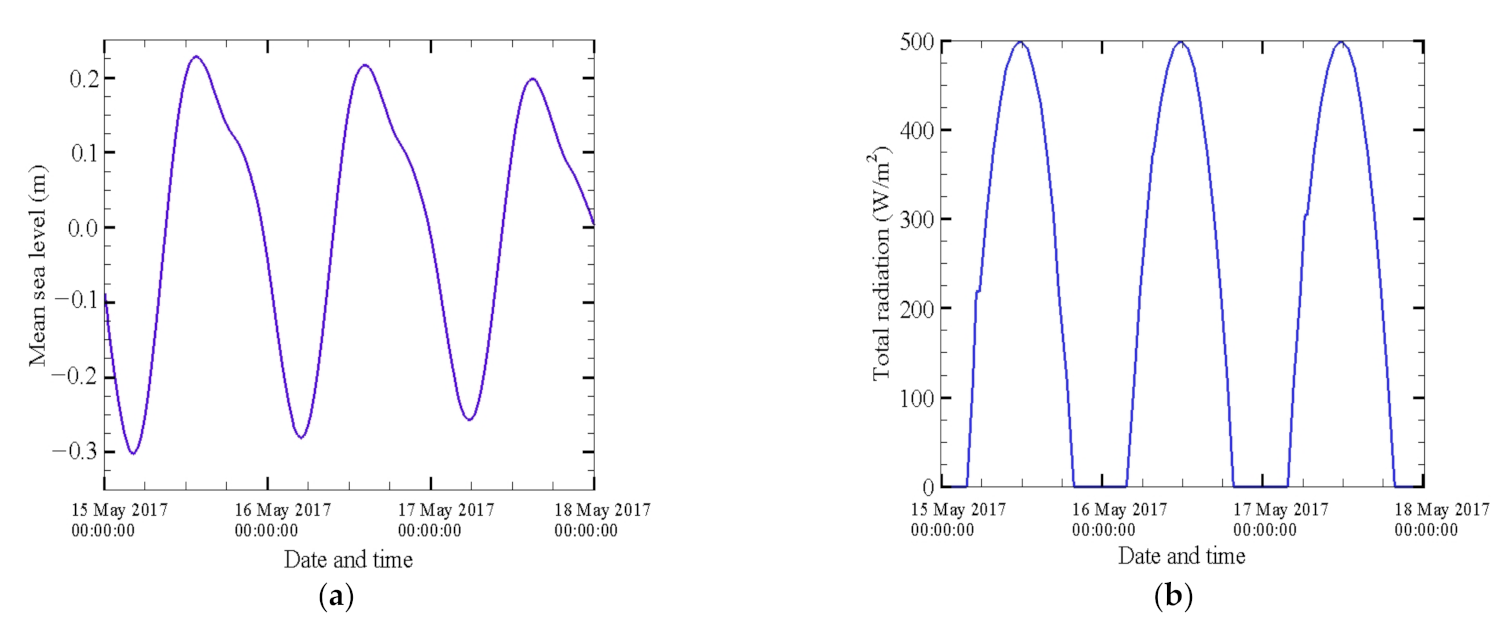
To expand the analysis of the thermal plume emitted by the LVNPP, numerical simulations were calibrated and validated with the aid of RS temperature fields. For this purpose, only the scenario of Figure 8b was simulated, as it is a nonfavorable scenario for the performance of the power plant, as mentioned above. To match the scenario of RS for the spring season on 17 May 2017, the simulation period was configured from 15 May 2017 at 00:00 h to 17 May 2017 at 11:00 h, leaving two previous days for warm-up. The initial and boundary conditions are detailed in Section 2.5. The scenario was reproduced with the AEM and the $k-L$ and $k-\epsilon$ turbulence closure models, activating and deactivating the HLES scheme of Delft3D-FLOW, to carry out a discussion on the performance of each model. For simulations performed with HLES, the default sub-grid scale model setup parameters were considered. The temperature at the discharge was fixed to 35 °C, whereas the temperature of the suction at the intake structure was 29.4 °C, according to the RS temperature fields. Regarding the El Viejon river, a constant temperature of 30 °C was imposed.

A trial and error process that involved increasing and decreasing the parameters ${\nu }_H^{back},{\nu }_V^{back}, D_H^{back}$, and $D_V^{back}$ was applied for satisfactory agreement with the RS data, based on the following three metrics:

$$RMSE=\sqrt{\frac{{{\displaystyle \sum }}_{i=1}^n{\left[T_{RS}\left(i\right)-T_{sim}\left(i\right)\right]}^2}{n}},$$

(13)

$$NS=1-\frac{{{\displaystyle \sum }}_{i=1}^n{\left[T_{RS}\left(i\right)-T_{sim}\left(i\right)\right]}^2}{{{\displaystyle \sum }}_{i=1}^n{\left[T_{RS}\left(i\right)-\overline{T}\right]}^2},$$

(14)

$$m=\frac{{{\displaystyle \sum }}_{i=1}^n\left|T_{RS}\left(i\right)-T_{sim}\left(i\right)\right|}{{{\displaystyle \sum }}_{i=1}^n{T}_{RS}\left(i\right)},$$

(15)

where $RMSE$ is the root mean square error; m is the mass balance error; $T_{RS}$ and $T_{sim}$ are the RS and simulated temperatures, respectively; $\overline{T}$ is the mean of $T_{RS}$; $n$ is the number of monitoring points.

Table 5. Background calibration parameters for simulations.

Parameter	Value Range (m2/s)	Final Value (m2/s)
${\nu }_H^{back}$	10−5–102	0.002
${\nu }_V^{back}$	10−5–102	0.02
$D_H^{back}$	10−5–102	2
$D_V^{back}$	10−5–102	0.6

shows the final values used for the simulations. The background parameters are determinant to the variation in the results and are required to compute ${\nu }_H,{\nu }_{V,}{D}_H$, and $D_V$, as described by Equations (4), (5), (7) and (8), respectively.

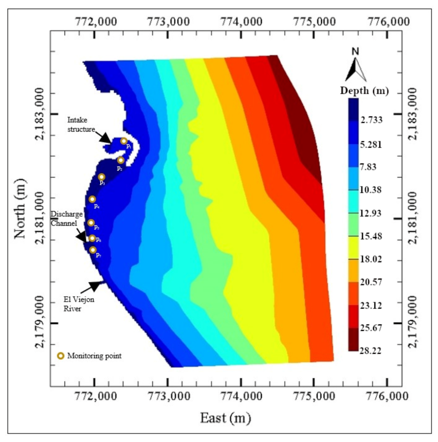
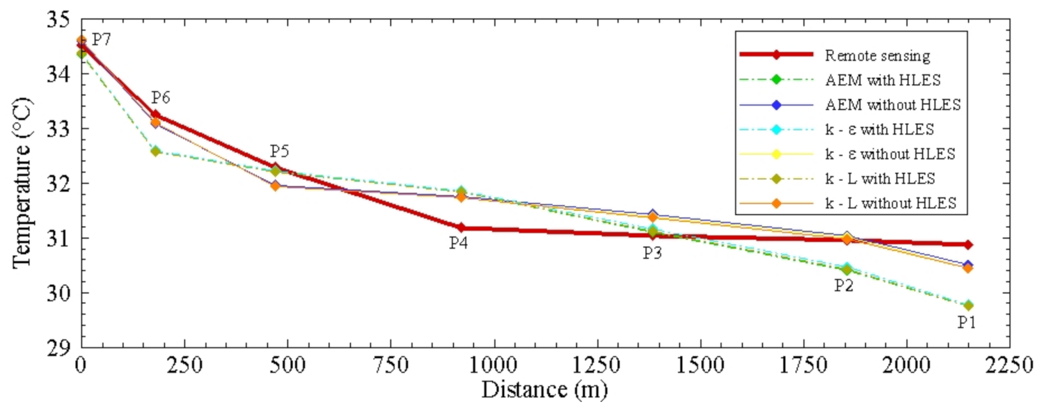
Figure 9 illustrates the temperature decay curves following the monitoring points, from P7, closest to the discharge, to P1, furthest from the discharge and closest to the intake structure (Figure 2). These results correspond to the date 17 May 2017 at 10:45 h, which is the time that matches the RS data of the same date (Figure 8b). The solid red line shows the temperature decay curve of the RS data, while the rest of the lines depict the simulated decay curves with the different turbulence closure models.

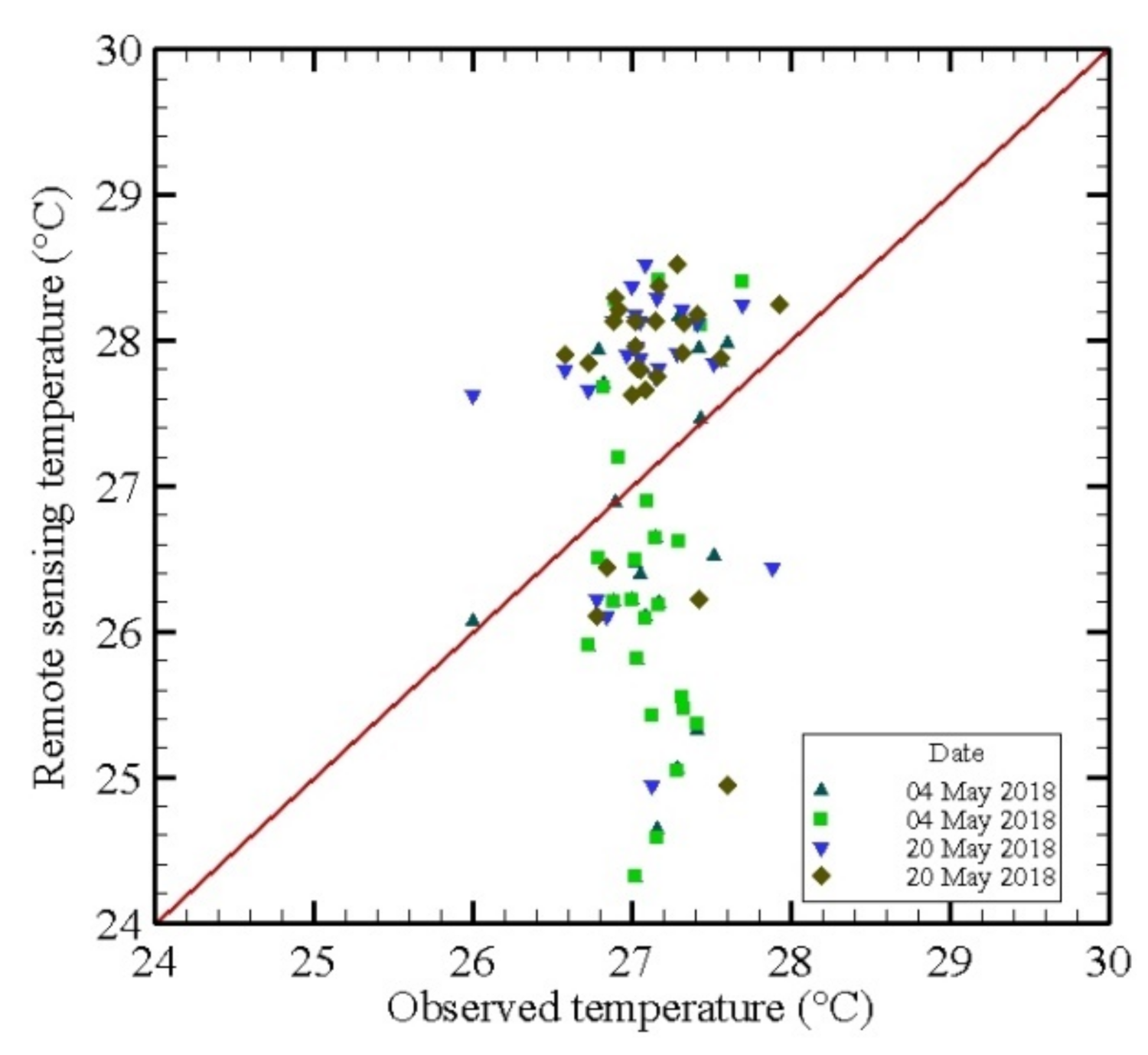
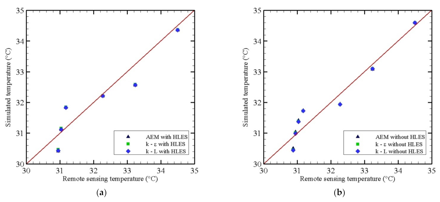
Figure 10 shows the dispersion of RS temperatures versus simulated temperatures obtained with the different turbulence closure models at each monitor point. It is evident that more data dispersion exists when using turbulence models with HLES (Figure 10a) compared with the ones without HLES (Figure 10b).

Table 6. Error criteria for each turbulence model.

Metric	With HLES			Without HLES
	AEM	$\mathit{k}-\mathit{L}$	$\mathit{k}-\mathit{\epsilon }$	AEM	$\mathit{k}-\mathit{L}$	$\mathit{k}-\mathit{\epsilon }$
$\mathrm{RMSE}$	0.598	0.594	0.585	0.334	0.334	0.333
$\mathrm{NS}$	0.788	0.791	0.797	0.934	0.934	0.934
$m$	0.014	0.014	0.014	0.009	0.009	0.009
B	0.248	0.239	0.218	−0.048	−0.022	−0.032

shows the corresponding errors of each simulation against the RS data. The values of the RMSE for the three turbulence closure models with HLES are around 0.59, whereas these values are lower without HLES, around 0.33. For the NS, the values with HLES for the three models are around 0.79, whereas they are around 0.93 without HLES. For the m criterion, calculations with HLES yield values of around 0.014, whereas these are around 0.009 without HLES. In general, better agreement is observed for the simulations without HLES, and, considering the calculated bias, the simulation with the $k-\epsilon$ turbulence model correlates best with the RS data.

In terms of the RMSE efficiency criterion, it may appear that some of the simulations are poorly consistent with the RS data; however, there are countless variables arising from different sources in the coastal zone, such as hydrological, meteorological, climatic, and oceanographic variables, which introduce complexity. The diversity in the temporal and spatial scales of these variables also generates a level of uncertainty. The study is therefore far from being a controlled experiment, so the RMSE correlation is acceptable in this case. On the other hand, for the NS efficiency criterion, good agreement is found with the RS data. According to [52], an NS efficiency score greater than 0.5 indicates acceptable numerical modeling performance. Regarding the m criterion, the values from both models (i.e., with and without HLES) are close to zero (0.014 and 0.009, respectively), indicating good approximation.

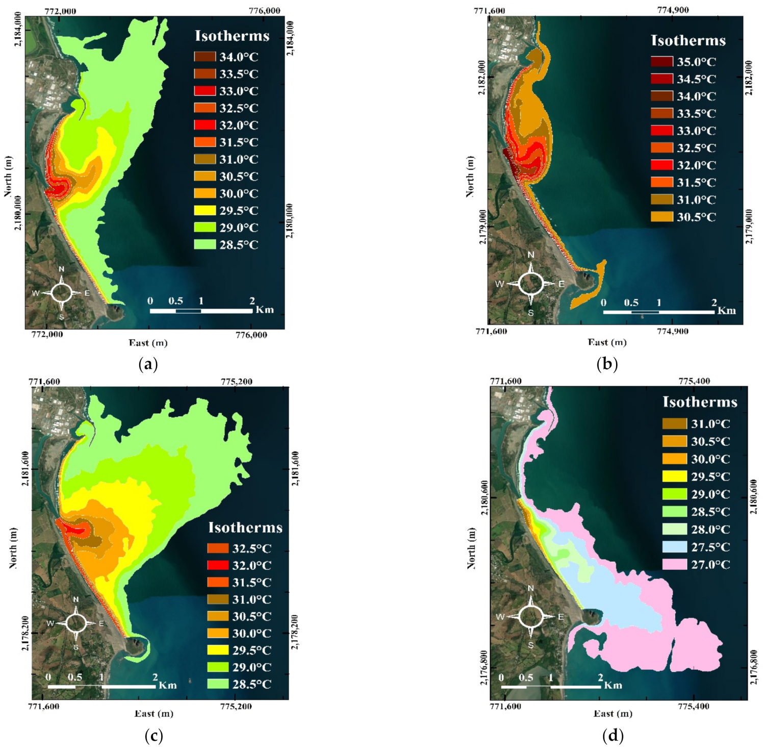
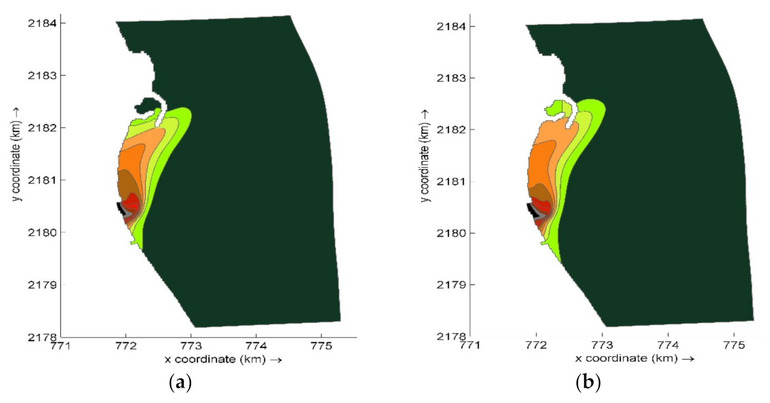
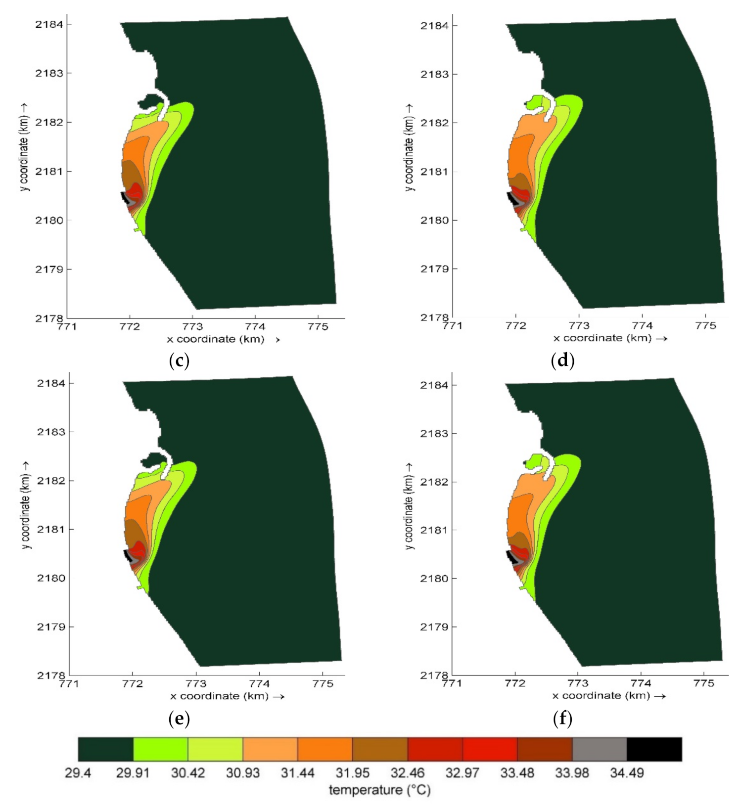
Figure 11 shows the simulated surface thermal fields of the above comparisons of the three turbulence closure models considered, with and without HLES. In general, the patterns of the simulated thermal plumes are in good agreement with those derived from the RS data (Figure 8b). The numerical simulations closely describe the dissipation of the plume towards the intake structure, the critical scenario for the performance of the power plant cooling system. Although the overall thermal fields are similar in all cases, the results without HLES yield greater temperature values in the intake structure, as represented by the isotherms. This means that, when activating the HLES model, the heat dissipates at a higher rate, compared with the simulations without HLES. In fact, the potential core of the thermal discharge reproduced with HLES simulations covers a smaller area than the one reproduced by simulations without HLES. Finally, from the temperature fields of each turbulence closure model, AEM, $k-L,$ and $k-\epsilon$, no differences were observed among them.

3.2.2. Thermal Plume Dispersion Analysis

The results shown in Section 3.2.1 are further discussed based on a behavioral analysis of several dimensionless numbers and variables.

Table 7. Definitions of dimensionless variables.

Variable	Formula
Dimensionless distance	$X^{*}=\frac{X_p}{W_C}$
Dimensionless horizontal velocity	$U^{*}=\frac{U}{U_{max}}$
Dimensionless temperature	$T^{*}=\frac{T}{T_{max}}$
Dimensionless vertical eddy viscosity	${\nu }_t^{*}=\frac{{\mathsf{\nu }}_{3D}}{{\mathsf{\nu }}_{3D_{max}}}$
Dimensionless turbulent energy	$k^{*}=\frac{k}{k_{max}}$
Dimensionless energy dissipation	${\epsilon }^{*}=\frac{\epsilon }{{\epsilon }_{max}}$
Reynold’s number	$R_e=\frac{U{W}_D}{{\nu }_{mol}}$
Densimetric Froude number	$F_{rd}=\frac{U}{\sqrt{g{W}_D\left(\frac{{\rho }_0-\rho }{{\rho }_0}\right)}}$
Grashof number	$G_r=\frac{g\beta \left(T_p-T_{\infty }\right)W_D^3}{{\nu }_{mol}^2}$
Peclet number	$P_e=R_e{P}_r$
Richardson’s number	$R_i=\frac{G_r}{R_e^2}$

shows the definition of each one, where $W_D$ and $W_C$ are the discharge channel depth and width at the outlet, respectively (m); $\beta$ is the volumetric expansion coefficient (1/°C); $T_{\infty }$ is the ambient temperature set to 29.4 °C; $P_{r }$is the Prandtl number, equal to $0.9$; ${\rho }_0$ is the standard seawater density, considered $1024 \mathrm{kg}/{\mathrm{m}}^3$;$X_p$ is the distance from P7 to the other monitoring points (m). The parameters$k_{max}$ (m²/s²), ${\epsilon }_{max}$, (m²/s³), ${\mathsf{\nu }}_{3D_{max}}$(m²/s), $T_{max}$(°C), and $U_{max}$ (m/s) are the maximum values calculated at the monitoring points.

The analyses are based on the results obtained for the monitoring points shown in Figure 2, and their coordinates can be found in Table 1.

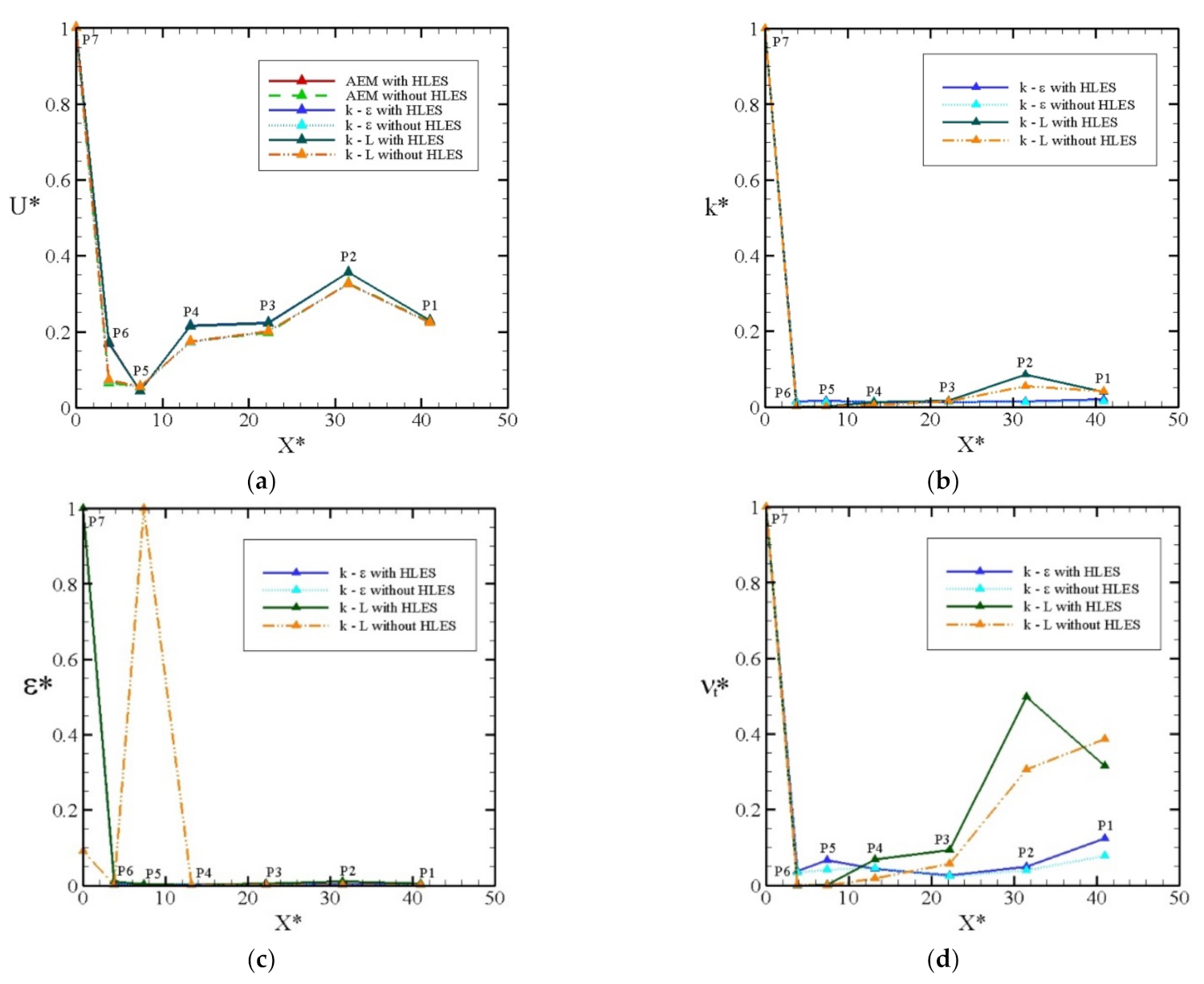
Figure 12 shows the evolution of the dynamic field from P7 to P1, following the plume trajectory. Figure 12a illustrates the evolution of $U^{*}$, whereas Figure 12b–d show the dimensionless turbulent parameters $k^{*}$, ${\epsilon }^{*}$, and ${\nu }_t^{*}$, respectively. One of the advantages provided by the $k-\epsilon$ model is that the transport of kinetic energy and its dissipation are calculated. The $k-L$ model does solve the kinetic energy transport equation; however, it does not solve the turbulent dissipation transport equation. To have an approximation of the turbulent dissipation when using the $k-L$ model, the semi-empirical relationship of Kolmogorov–Prandtl, Equation (9), was applied, although, as observed in Figure 12c,d, the results do not show coherence with those obtained from the $k-\epsilon$ model. The turbulent variables from the results of the AEM model were not calculated, since such a model does not even estimate the transport of kinetic energy. From the evolution of $U^{*}$, it was observed that, between P7 and P6, the thermal transport was dominated by advective processes arising from the momentum introduced by the discharge channel, whereas, between P5 and P1, it was dominated by diffusive processes, which govern the transport of the plume due to the force induced by surface wind shear and the inertia of the coastal marine currents. Regarding Figure 12b–d, between P7 and P6, the decrease in the turbulence parameters is dominated by the momentum induced by the flow in the channel discharge. This is the area in which the turbulence, and consequently the dissipation, is highest. Between P6 and P1, the evolution of the turbulence parameters is dominated by diffusive processes induced by both the velocities and the temperature in the far field. There are differences between the calculations with and without HLES in the same way as there are in the mean flow.

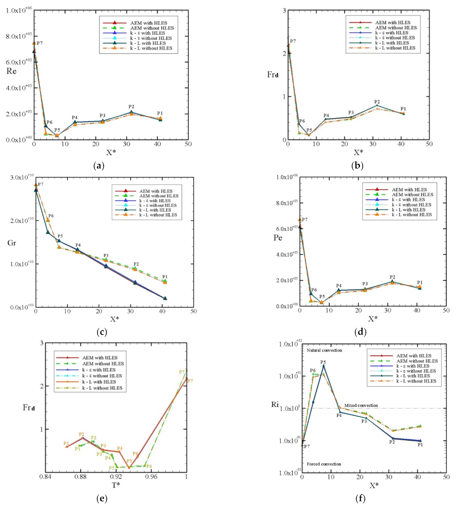
Figure 13 shows the evolution and impact of the thermal plume, including a comparison of dimensionless numbers that relate inertial and viscous force effects, natural and forced convection, heat transfer and thermal diffusion, and finally density and buoyancy effects [53]. Overall, the values from the models with HLES are higher than those without HLES, since an additional eddy viscosity is introduced by ${\nu }_{SGS}$. The variation of $R_e$ with $X^{*}$ is shown in Figure 13a. In general, inertial forces predominate over viscous ones. It is worth mentioning that, from P7 to P6, higher values of $Re$ are observed; this is expected, since the highest velocities are found near the discharge. The evolution of $F_{rd}$ with $X^{*}$ is shown in Figure 13b. Near the discharge, inertial forces predominate over buoyancy ones up to P5. After this point, an equilibrium is observed between these two forces, with buoyancy forces slightly predominating over inertial ones, since the values of $F_{rd}$ are lower than one. Figure 13c shows a plot of $G_r$ versus $X^{*}$. The highest temperature gradients are found between P7 and P6, and, as expected, the highest values for $G_r$ are observed at these points. From P6 to P1, the values of $G_r$ are smoothly reduced as the thermal plume approaches the intake structure. Overall, buoyancy forces dominate over viscous ones. The variation of $P_e$ is shown in Figure 13d. Between P7 and P6, a predominance of convective forces over diffusive ones is observed, due to the momentum introduced by the discharge channel. Although the $P_e$ curves drop down significantly at the remaining points, the process remains dominated by convective forces since the diffusive ones are not strong enough to counteract them. Figure 13e illustrates the relationship between $F{r}_d$and $T^{*}$. Between P7 and P5, inertial forces predominate over viscous and buoyancy forces. From P5 to P1, an increase in the buoyancy forces tends to counteract the inertial forces, since the curves tend towards $F{r}_d$ = 1.

Figure 13f shows an analysis of the forced and natural convection. The following criterion is used to classify the convective heat transfer mode of the flow [54]. If $R_i\gg$ 1, natural convection effects dominate; if $R_i\ll$ 1, buoyancy forces are negligible, and forced convection must be considered; when $R_i\approx$ 1, the flow is referred to as a mixed convection. Due to the influence of the discharge, in P7, $R_i<1$, but not to the degree at which forced convection dominates over natural convection. Between P6 and P4, $R_i>1$, but again, not to the degree at which natural convection dominates over forced convection. Because of the influence at the intake structure, $R_i$ tends towards values lower than 1 at monitors P4 to P1, but still, in a regime where it is difficult to infer, forced convection dominates the process. Thus, given the behavior of $R_i$, a mixed convection regime can be implied on all the monitor points, because the values of $R_i$ are not much higher or much lower than 1, a condition that evidences the predominance of forced or natural convection in the thermal process.

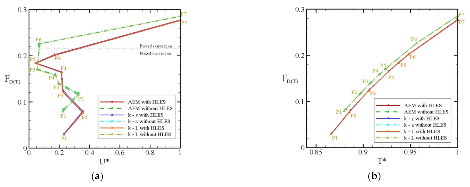
To determine the mode that dominates the heat transfer in the thermal plume dispersion, forced or natural convection, along the monitoring points, a dimensionless quantity was introduced as

$$F_{D\left(T\right)}=\beta {\rho }_0\frac{∆T}{∆\rho }.$$

(16)

This factor is a metric of density variations because it reflects the dimensionless density bias due to linear dilatation with respect to the reference density ${\rho }_0$. In cases such as the one analyzed here, where the density variations due to temperature (dilatation) are small, this relationship helps to represent such variations in orders of magnitude close to 1. With this, whether force convection or natural convection dominates over the other in the thermal process can be observed.

Figure 14 shows the behavior of $F_{D\left(T\right)}$ regarding $U^{*}$ and $T^{*}$. Figure 14a tries to illustrate the limits of forced and natural convection along the monitoring points, by comparing $F_{D\left(T\right)}$ versus $U^{*}$. From P7 to P6, in the near discharge area, $F_{D\left(T\right)}$ depends on the velocity variation, which means that gradients of $F_{D\left(T\right)}$ over velocity gradients yield values of the order of magnitude close to 1. This region can be inferred as dominated by forced convection. From monitor points P5 to P1, the behavior is different, because the process is not dependent on the velocity variation, which means that gradients of $F_{D\left(T\right)}$ over velocity gradients would yield very small values, a much lower order of magnitude than 1. Thus, this region is dominated by mixed convection. Figure 14b illustrates the relationship $F_{D\left(T\right)}$ versus $T^{*}$, in which the behavior is almost linear. The curve shows that, as $T^{*}$ decreases from P7 to P1, $F_{D\left(T\right)}$ also decreases, which means that, as the temperature becomes colder, the density bias decreases. This only evidences the good agreement of the behavior of $F_{D\left(T\right)}$ with the behavior of the thermodynamic state of the system.

4. Conclusions

This work focused on studying the marine dispersion of a thermal plume from a nuclear power plant. Firstly, an RS analysis was conducted, and a numerical simulation analysis of a particular case was then carried out. Based on the numerical simulation results, the work ends with a comparison of three turbulence closure models and with an analysis of nondimensional parameters to explain the thermal dispersion process. The case study was a complex dynamic scenario driven by tides and winds.

The RS analysis was conducted for different scenarios: winter, spring, summer, and fall seasons. This technique was calibrated and validated with the aid of field measurements of a wide spatial region. Results showed that, though the plume disperses far away from the intake structure, temperature disturbances at the intake caused by the discharge are still observed. This fact is highly undesirable because the power plant’s performance is compromised.

Numerical simulations were carried out to reproduce the behavior of the thermal plume for the scenario shown in Figure 8b, in which the plume disperses towards the intake of the power plant. The RS results served to calibrate the numerical model because of the lack of field measurements in the plume influence area. The calibration results showed good agreement with the RS data based on the applied metrics (Table 5). After model calibration, the results of three different turbulence closure models—AEM and the $k-L$ and $k-\epsilon$ models—were compared. In general, the results of the three turbulence closure models applied showed similar values of the dimensionless parameters compared. For quantities such as ${\nu }_t^{*}$ and ${\epsilon }^{*}$, the results of the $k-L$ model were not satisfactory, since it overpredicts the turbulence quantities, compared with the $k-\epsilon$ model. In addition, the three error criteria showed the least error when using the $k-\epsilon$ model; thus, according to these two findings, the $k-\epsilon$ model can be considered to have performed best among the three turbulence closure models applied for the case study. On the other hand, while using the HLES scheme, the compared dimensionless parameters showed different patterns. The area covered by thermal plumes estimated with HLES is smaller than the ones estimated by simulations without HLES. These differences can be attributed to the HLES theoretical background, which is specific for 2D simulations.

The results from analysis of both the hydrodynamic and thermal variables were consistent. For the hydrodynamic variables, it was observed that, at the outset, the plume is dominated by inertial processes due to the momentum induced in the discharge channel, and that it is later dominated by diffusive processes that are associated with the properties and characteristics of the coastal zone (Figure 13). The dimensionless number $F_{D\left(T\right)}$ showed that, close to the discharge, the thermal transport is dominated by forced convection induced by the discharge. In the far field, the thermal transport is dominated by mixed convection associated with the properties and characteristics of the sea in the coastal zone.

Finally, the combination of different techniques to analyze the behavior of thermal plume dispersion into the sea, RS and numerical simulation in this case, provides a better understanding of the phenomenon, regarding spatial effects from the perspective of power plant performance and low environmental impacts. With a lack of local field measurements, the use of RS calibrated with field measurements of an extended area was a good alternative to calibrate and validate numerical simulations in the local influence area of the thermal plume.

References

1. Kirillin, G.; Shatwell, T.; Kasprzak, P. Consequences of Thermal Pollution from a Nuclear Plant on Lake Temperature and Mixing Regime. J. Hydrol. 2013, 496, 47–56. [Google Scholar] [CrossRef]
2. Li, X.Y.; Li, B.; Sun, X.L. Effects of a Coastal Power Plant Thermal Discharge on Phytoplankton Community Structure in Zhanjiang Bay, China. Mar. Pollut. Bull. 2014, 81, 210–217. [Google Scholar] [CrossRef]
3. Azmi, S.; Agarwadkar, Y.; Bhattacharya, M.; Apte, M.; Inamdar, A.B. Monitoring and Trend Mapping of Sea Surface Temperature (SST) from MODIS Data: A Case Study of Mumbai Coast. Environ. Monit. Assess. 2015, 187, 165. [Google Scholar] [CrossRef] [PubMed]
4. Jan, S.; Chen, C.T.A.; Tu, Y.Y.; Tsai, H.S. Physical Properties of Thermal Plumes from a Nuclear Power Plant in the Southernmost Taiwan. J. Mar. Sci. Technol. 2004, 12, 433–441. [Google Scholar] [CrossRef]
5. Colinvaux, P. Life at low Reynold’s number. Nature 1979, 277, 353–354. [Google Scholar] [CrossRef]
6. Li, N.; Mao, Z.; Zhang, Q.; Wang, D.; Bai, Y.; Pan, D. The Numerical Simulation and Remote Sensing of the Thermal Discharge from the Qinshan Nuclear Power Station. In Proceedings of the SPIE Asia-Pacific Remote Sensing, Noumea, New Caledonia, 17–21 November 2008; Volume 7150. [Google Scholar] [CrossRef]
7. Zoran, M.A.; Savastru, R.S.; Savastru, D.M.; Miclos, S.I.; Tautan, M.N.; Baschir, L.V. Thermal Pollution Assessment in Nuclear Power Plant Environment by Satellite Remote Sensing Data. In Proceedings of the SPIE Asia-Pacific Remote Sensing, Edinburgh, UK, 8-12 November 2012; Volume 8531, p. 853120. [Google Scholar] [CrossRef]
8. Zhang, Z.; He, G.; Wang, M.; Long, T.; Wang, G.; Zhang, X.; Jiao, W. Towards an Operational Method for Land Surface Temperature Retrieval from Landsat 8 Data. Remote Sens. Lett. 2016, 7, 279–288. [Google Scholar] [CrossRef]
9. Bonansea, M.; Ferrero, S.; Ferral, A.; Ledesma, M.; German, A.; Carreño, J.; Rodriguez, C.; Pinotti, L. Assessing Water Surface Temperature from Landsat Imagery and Its Relationship with a Nuclear Power Plant. Hydrol. Sci. J. 2021, 66, 50–58. [Google Scholar] [CrossRef]
10. Issakhov, A. Mathematical Modeling of the Discharged Heat Water Effect on the Aquatic Environment from Thermal Power Plant under Various Operational Capacities. Appl. Math. Model. 2016, 40, 1082–1096. [Google Scholar] [CrossRef]
11. Jia, H.l.; Zheng, S.; Xie, J.; Ying, X.m.; Zhang, C.p. Influence of Geographic Setting on Thermal Discharge from Coastal Power Plants. Mar. Pollut. Bull. 2016, 111, 106–114. [Google Scholar] [CrossRef]
12. Shah, V.; Dekhatwala, A.; Banerjee, J.; Patra, A.K. Analysis of Dispersion of Heated Effluent from Power Plant: A Case Study. Sadhana Acad. Proc. Eng. Sci. 2017, 42, 557–574. [Google Scholar] [CrossRef] [Green Version]
13. Deabes, E.A.M. The Impact of Thermal Power Stations on Coastline and Benthic Fauna: Case Study of El-Burullus Power Plant in Egypt. Results Eng. 2020, 7, 100128. [Google Scholar] [CrossRef]
14. Gaeta, M.G.; Samaras, A.G.; Archetti, R. Numerical Investigation of Thermal Discharge to Coastal Areas: A Case Study in South Italy. Environ. Model. Softw. 2020, 124, 104596. [Google Scholar] [CrossRef]
15. Yu, L.; Yu, J. Numerical Research on Flow and Thermal Transport in Cooling Pool of Electrical Power Station Using Three Depth-Averaged Turbulence Models. Water Sci. Eng. 2009, 2, 1–12. [Google Scholar] [CrossRef]
16. Lunis, M.; Mamchuk, V.; Movchan, V.; Romanyuk, L.; Shkvar, E. Algebraic Models of Turbulent Viscosity and Heat Transfer in Analysis of Near-Wall Turbulent Flows. Int. J. Fluid Mech. Res. 2004, 31, 60–74. [Google Scholar] [CrossRef]
17. Furue, R.; Jia, Y.; McCreary, J.P.; Schneider, N.; Richards, K.J.; Müller, P.; Cornuelle, B.D.; Avellaneda, N.M.; Stammer, D.; Liu, C.; et al. Impacts of Regional Mixing on the Temperature Structure of the Equatorial Pacific Ocean. Part 1: Vertically Uniform Vertical Diffusion. Ocean Model. 2015, 91, 91–111. [Google Scholar] [CrossRef] [Green Version]
18. Ali, J.; Fieldhouse, J.; Talbot, C. Turbulent Cooling Water Discharge into Still Body of Water. Nucl. Eng. Des. 2011, 241, 2006–2012. [Google Scholar] [CrossRef]
19. Kumar, R.; Dewan, A. Computational Models for Turbulent Thermal Plumes: Recent Advances and Challenges. Heat Transf. Eng. 2014, 35, 367–383. [Google Scholar] [CrossRef]
20. Verma, M.K.; Kumar, A.; Pandey, A. Phenomenology of Buoyancy-Driven Turbulence: Recent Results. New J. Phys. 2017, 19, 025012. [Google Scholar] [CrossRef]
21. Burchard, H.; Craig, P.D.; Gemmrich, J.R.; van Haren, H.; Mathieu, P.P.; Meier, H.E.M.; Smith, W.A.M.N.; Prandke, H.; Rippeth, T.P.; Skyllingstad, E.D.; et al. Observational and Numerical Modeling Methods for Quantifying Coastal Ocean Turbulence and Mixing. Prog. Oceanogr. 2008, 76, 399–442. [Google Scholar] [CrossRef]
22. James, I.D. Modelling Pollution Dispersion, the Ecosystem and Water Quality in Coastal Waters: A Review. Environ. Model. Softw. 2002, 17, 363–385. [Google Scholar] [CrossRef]
23. Chen, Q.; Xu, W. A Zero-Equation Turbulence Model for Indoor Airflow Simulation. Energy Build. 1998, 28, 137–144. [Google Scholar] [CrossRef]
24. Rodi, W. Turbulence Modeling and Simulation in Hydraulics: A Historical Review. J. Hydraul. Eng. 2017, 143, 1–20. [Google Scholar] [CrossRef]
25. Hinterberger, C.; Froehlich, J.; Rodi, W. Three-dimensional and depth-averaged Large-Eddy Simulations of Some Shallow.Water Flows. J. Hydraul. Eng. 2007, 133, 857–872. [Google Scholar] [CrossRef]
26. Silva, H.A.; Botello, A.V. Evaluación del Impacto ambiental de la central Nucleoléctrica Laguna Verde. In Golfo de México. Contaminación e Impacto Ambiental: Diagnóstico y Tendencias; EPOMEX: Campeche, Mexico, 1996. [Google Scholar]
27. Botello, A.V.; Rendón, J. Evaluación del Impacto ambiental de la central Nucleoléctrica Laguna Verde a 15 años de operación. In Golfo de México. Contaminación e Impacto Ambiental: Diagnóstico y Tendencias; EPOMEX: Campeche, Mexico, 2005. [Google Scholar]
28. Ramírez-León, H.; Couder-Castañeda, C.; Herrera-Díaz, I.E.; Barrios-Piña, H.A. Modelación Numérica de La Descarga Térmica de La Central Nucleoeléctrica Laguna Verde. Rev. Int. Metod. Numer. Calc. Disen. Ing. 2013, 29, 114–121. [Google Scholar] [CrossRef] [Green Version]
29. Roelvink, J.A.; Van Banning, G.K.F.M. Design and development of DELFT3D and application to coastal morphodynamics. In Hydroinformatics; Verwey, A., Minns, A.W., Babovic, V., Maksimovic, C., Eds.; Balkema: Rotterdam, The Netherlands, 1994; pp. 451–456. [Google Scholar]
30. Lesser, G.R.; Roelvink, J.A.; van Kester, J.A.T.M.; Stelling, G.S. Development and Validation of a Three-Dimensional Morphological Model. Coast. Eng. 2004, 51, 883–915. [Google Scholar] [CrossRef]
31. Gerritsen, H.; de Goede, E.D.; Platzek, F.W.; Genseberger, M.; van Kester, J.A.T.M.; Uittenbogaard, R.E. Validation Document Delft3D-FLOW: A Software System for 3D Flow Simulations; Deltares: Delft, The Netherlands, 2007; p. 266. [Google Scholar]
32. De Graaff, R.; Lindfors, A.; De Goede, E.; Rasmus, K.; Morelissen, R. Modelling of a Thermal Discharge in an Ice-Covered Estuary in Finland. In Proceedings of the OTC Arctic Technology Conference, Copenhagen, Denmark, 23–25 March 2015; pp. 488–506. [Google Scholar] [CrossRef]
33. Sana, A. Hydrodynamic and Thermal Dispersion Modelling of the Effluent in a Coastal Channel. In Recent Progress in Desalination, Environmental and Marine Outfall Systems, 1st ed.; Baawain, M., Choudri, B., Ahmed, M., Purnama, A., Eds.; Springer: Cham, Switzerland, 2015; pp. 269–283. [Google Scholar] [CrossRef]
34. Vroom, J.; van der Wegen, M.; Martyr-Koller, R.C.; Lucas, L.V. What Determines Water Temperature Dynamics in the San Francisco Bay-Delta System? Water Resour. Res. 2017, 53, 9901–9921. [Google Scholar] [CrossRef]
35. Deltares. Delft3D-FLOW User Manual, 3.15 ed.; Deltares: Delft, The Netherlands, 2020. [Google Scholar]
36. Smagorinsky, J. General circulation experiments with the primitive equations. I: The basic experiment. Mon. Weather Rev. 1963, 91, 99–164. [Google Scholar] [CrossRef]
37. Uittenbogaard, R.; vanVossen, B. Subgrid-scale model for quasi-2D turbulence in shallow water. In Shallow Flows; Jirka, G., Uijttewaal, W., Eds.; Taylor & Francis Group: London, UK, 2004; pp. 575–582. [Google Scholar]
38. García, R. Análisis de Dispersión de la Pluma Térmica de la Central Nucleoeléctrica Laguna Verde Mediante Teledetección. Master’s Thesis, Universidad Autónoma del Estado de México, Mexico City, Mexico, 16 December 2020. [Google Scholar] [CrossRef]
39. Ramírez-León, H.; Barrios-Piña, H.; Torres-Bejarano, F.; Cuevas-Otero, A.; Rodríguez-Cuevas, C. Numerical Modelling of the Laguna Verde Nuclear Power Station Thermal Plume Discharge to the Sea. In High Performance Computer Applications, 1st ed.; Gliter, I., Klapp, J., Eds.; Springer International Publishing: Cham, Switzerland, 2016; pp. 495–507. [Google Scholar] [CrossRef]
40. Stelling, G.; Leendertse, J. Approximation of convective processes by cyclic AOI methods. In Estuarine and Coastal Modeling; Spaulding, M., Bedford, K., Blumberg, A., Eds.; American Society of Civil Engineers: Tampa, FL, USA, 1992; pp. 771–782. [Google Scholar]
41. Ghani, A.A.; Zakaria, N.A.; Kiat, C.C.; Ariffin, J.; Hasan, Z.A.; Abdul Ghaffar, A.B. Revised Equations for Manning’s Coefficient for Sand-Bed Rivers. Int. J. River Basin Manag. 2007, 5, 329–346. [Google Scholar] [CrossRef] [Green Version]
42. Durán-Colmenares, A.; Barrios-Piña, H.; Ramírez-León, H. Numerical Modeling of Water Thermal Plumes Emitted by Thermal Power Plants. Water 2016, 8, 482. [Google Scholar] [CrossRef] [Green Version]
43. Archivo de Tiempo en Veracruz (Aeropuerto), METAR. Available online: https://rp5.ru/Archivo_de_tiempo_en_Veracruz_(aeropuerto),_METAR (accessed on 13 October 2020).
44. USGS EarthExplorer. Available online: https://earthexplorer.usgs.gov/ (accessed on 20 July 2020).
45. Yu, X.; Guo, X.; Wu, Z. Land Surface Temperature Retrieval from Landsat 8 TIRS-Comparison between Radiative Transfer Equation-Based Method, Split Window Algorithm and Single Channel Method. Remote Sens. 2014, 6, 9829–9852. [Google Scholar] [CrossRef] [Green Version]
46. Snyder, J.; Boss, E.; Weatherbee, R.; Thomas, A.C.; Brady, D.; Newell, C. Oyster Aquaculture Site Selection Using Landsat 8-Derived Sea Surface Temperature, Turbidity, and Chlorophyll A. Front. Mar. Sci. 2017, 4, 190. [Google Scholar] [CrossRef] [Green Version]
47. USGS. Landsat 8 (L8) Data Users Handbook; Version 5; Department of the Interior, U.S. Geological Survey: Reston, VA, USA, 2019.
48. Allen, R.G.; Tasumi, M.; Morse, A.; Trezza, R.; Wright, J.L.; Bastiaanssen, W.; Kramber, W.; Lorite, I.; Robison, C.W. Satellite-Based Energy Balance for Mapping Evapotranspiration with Internalized Calibration (METRIC)—Applications. J. Irrig. Drain. Eng. 2007, 133, 395–406. [Google Scholar] [CrossRef]
49. Wukelic, G.E.; Gibbons, D.E.; Martucci, L.M.; Foote, H.P. Radiometric Calibration of Landsat Thematic Mapper Thermal Band. Remote Sens. Environ. 1989, 28, 339–347. [Google Scholar] [CrossRef]
50. Newman, S.M.; Smith, J.A.; Glew, M.D.; Rogers, S.M.; Taylor, J.P. Temperature and Salinity Dependence of Sea Surface Emissivity in the Thermal Infrared. Q. J. R. Meteorol. Soc. 2005, 131, 2539–2557. [Google Scholar] [CrossRef]
51. Telford, R.J.; Birks, H.J.B. The Secret Assumption of Transfer Functions: Problems with Spatial Autocorrelation in Evaluating Model Performance. Quat. Sci. Rev. 2005, 24, 2173–2179. [Google Scholar] [CrossRef]
52. Knoben, W.J.M.; Freer, J.E.; Woods, R.A. Technical Note: Inherent Benchmark or Not? Comparing Nash-Sutcliffe and Kling-Gupta Efficiency Scores. Hydrol. Earth Syst. Sci. 2019, 23, 4323–4331. [Google Scholar] [CrossRef] [Green Version]
53. Bezuglyi, B.A.; Ivanova, N.A.; Sizova, L.V. Transport Phenomena and Dimensionless Numbers: Towards a New Methodological Approach. Eur. J. Phys. 2017, 38, 033001. [Google Scholar] [CrossRef]
54. Çengel, Y.; Cimbala, J.; Turner, R. Fundamentals of Thermal-Fluid Sciences, 5th ed.; McGraw Hill Education: New York, NY, USA, 2017; pp. 828–829. [Google Scholar]
Figure 1. Location of the Laguna Verde nuclear power plant, Mexico.
Jmse 09 01437 g001
Figure 2. Bathymetry of the computational domain and monitoring points.
Jmse 09 01437 g002
Figure 3. NS score obtained and CPU time for mesh independence analysis.
Jmse 09 01437 g003
Figure 4. Grid and boundary conditions used in the numerical simulations.
Jmse 09 01437 g004
Figure 5. Metocean data: (a) tidal variation; (b) total solar radiation; (c) wind rose for the simulation period (wind speed in m/s).
Jmse 09 01437 g005aJmse 09 01437 g005b
Figure 6. SEMAR’s temperature measurement locations.
Jmse 09 01437 g006
Figure 7. Linear regression of the four images used for the validation process.
Jmse 09 01437 g007
Figure 8. Isotherms obtained from RS: (a) winter, 25 January 2017; (b) spring, 17 May 2017; (c) summer, 19 September 2016; (d) fall, 8 October 2017.
Jmse 09 01437 g008
Figure 9. Simulated decay temperature curves following the monitoring points P1 to P7, after the calibration and validation process with the RS data.
Jmse 09 01437 g009
Figure 10. Data dispersion between RS temperatures and simulated temperatures at monitor points for different turbulence closure models: (a) with HLES; (b) without HLES.
Jmse 09 01437 g010
Figure 11. Comparison of the free surface temperature at 10:45:00 on 17 May 2017 with several turbulence closure models: (a) AEM with HLES; (b) AEM without HLES; (c) k ε with HLES; (d) k ε without HLES; (e) k L with HLES; (f) k L without HLES.
Jmse 09 01437 g011aJmse 09 01437 g011b
Figure 12. Evolution from P7 to P1 of (a) U * ; (b) k * ; (c) ε * ; (d) ν t * .
Jmse 09 01437 g012
Figure 13. Evolution from P7 to P1 of the dimensionless numbers computed at the free surface for the turbulence closure models considered: (a) R e ; (b) F r d ; (c) G r ; (d) P e ; (e) F r d vs. T * ; (f)   R i .
Jmse 09 01437 g013
Figure 14. Behavior of the dimensionless parameter F D T computed at the free surface for the different turbulence closure models considered: (a) F D T vs. U * ; (b) F D T vs. T * .
Jmse 09 01437 g014