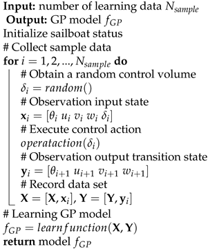
Article

Predictive Course Control and Guidance of Autonomous Unmanned Sailboat Based on Efficient Sampled Gaussian Process

College of Information Science and Technology, Donghua University, Shanghai 201620, China
*
Author to whom correspondence should be addressed.
J. Mar. Sci. Eng. 2021, 9(12), 1420; https://doi.org/10.3390/jmse9121420
Submission received: 1 November 2021 / Revised: 8 December 2021 / Accepted: 9 December 2021 / Published: 12 December 2021
(This article belongs to the Section Ocean Engineering)

Abstract

:
In view of the vulnerability of ocean unmanned sailboats to the large lateral velocities due to wind and waves during navigation, this paper proposes a Gaussian Process Model Predictive Control (GPMPC) method based on data-driven learning technique to improve the navigation tracking accuracy of unmanned sailboats. The feature model of the sailing course change subject to the wind and waves is learned from the efficient sampling data. It is then combined with the model predictive control to form the course controller. To reduce the influence of wind and waves disturbances, an adaptive weight term is designed in the object function to improve the tracking accuracy of the model predictive control. The guidance commands received by the model predictive controller take into account the path deviation caused by the current and lateral motion of the ship. The results show that GPMPC has the advantages of fast response time and less overshoot; the unmanned sailboat can better achieve waypoint tracking by learning navigation data.

1. Introduction

1.1. Background

With the exhaustion of terrestrial resources, the explored and exploitation of the ocean have gained increasing attention from researchers, governments and the military. In particular, the harsh and changeable marine environment, as well as the competitive situation, pose challenges to the continuous marine monitoring. In this context, an Unmanned Surface Vehicle (USV) as a maritime vehicle becomes in urgent need. In the complex water environment, USV can perform a variety of tasks such as, ocean reconnaissance, hydrological observation, etc. [1]. At the same time, the unmanned and energy-saving marine transportation has also gained more focus [2]. It requires USV to have the characteristics of large range, low energy consumption and long working time. Wind, as a widespread energy source in nature, is more likely to be used as a driving energy in an ocean-level environment without obstacles, which gives sailing ships a natural advantage in maritime navigation and continuous ocean observation. Compared with the conventional fuel-driven or electric drives, it can sail months of time with only a small amount of electricity [3]. Besides, the design and building of sailboats are simple and inexpensive. The study of unmanned sailboats is becoming a hot topic of extensive research worldwide [4]. However, the additional sail structure required for wind power drive make the motion characteristics and kinetics model of the sailboat complicated. Due to the uneven force of the sail exerted on the hull, the sailboat shows different response characteristics in different course angle. Compared with the traditional USV with a rear propeller, the sailboat may be disturbed by wind and waves, and thus it has a larger lateral speed and a roll angle when the sailboat operates in the ocean [5]. Additionally, the magnitude and direction of the sailing speed are directly affected by the wind speed and direction. It results in a re-design for the navigation approach of the sailboat. Considering the uniqueness of sailboats, the controller developed for the conventional USV cannot be applied to the sailboat directly, which brings new directions and challenges to the research of sailboat control.

1.2. Related Works

At present, related works of a sailboat mainly focus on the motion control and navigation. In terms of motion control, sailboats are independent of each other in the forward channel and the steering of yaw angle compared with most conventional guidance controllers, and the control of sailboats is often decomposed into the speed-related sail control and the course-related rudder control [6]. Since the wind cannot be predicted in the environment, researchers have paid more attention to the sailboat speed optimization mostly. Corno et al. [7] propose a data-based approach to design an extremum optimizer for sail control. Abrougui et al. [8] introduce a strategy to calculate the open sail angle using decoupled control. Júnior et al. [9] control the sail angle by designing fuzzy rules. However, the performance of various sail controllers is more or less the same due to wind limitation. Moreover, focus has been paid to the course controller design based on the sailing boat’s dynamic characteristics, and a large number of previous studies have been made in the course control of underdriven ships, including LQR (Linear Quadratic Regulator) and MPC (Model Predictive Control) in conventional optimal control, nonlinear controllers such as sliding mode control and backstepping control, and various intelligent control methods [10]. All these methods provide ideas for the controller design of sailboats. Among them, Zhang et al. [11] and He et al. [12] have introduced the backstepping method to control the ship’s heading angle. Furthermore, Deng et al. [13] also combine the traditional backstepping control method with the fuzzy logic system to reduce the complexity of the trajectory tracking controller. Xiao et al. [14] employ a sliding mode control with a simpler form to enhance the trajectory tracking performance of an underactuated USV. In addition, Cui et al. [15] have developed an adaptive sliding mode controller based on second-order dynamics of the underwater vehicle, which enable the controller to cope with effects due to the disturbances and the magic mismatch. Besides, a sliding mode controller based on a RBF neural network has been designed to predict the position by Zhang et al. [16], which also has a good effect on the heading control of large ships. Only that the methods mentioned above require the developer to be familiar with the ship model, such as calculation of fluid coefficient and added mass of ship, which brings more difficulty to the design of the unmanned sailboat. When the model cannot be described clearly, Zhou et al. [17] and Cruz and Alves [18] propose the self-tuning PID controllers, respectively. Furthermore, Yan et al. [19] have also designed the error-based nonlinear feedback controller to guide the saildrone. In order to improve the autonomy and the intelligence of the USV, Yunsheng et al. [20], as well as Deng et al. [21] designed fuzzy rules to improve the control the heading angle. Borkowski [22] also designed an expert system for large ships to resist ocean wind and wave interference. In addition, Astrov and Udal [23], Mu et al. [24], and Deng et al. [25] propose a neural network-based course control approach to guide the vehicle.
When developing the guidance law for the course control, the control method based on mathematical model can be adopted on the premise that the model of the sailboat is established in advance. Wind tunnel test or CFD simulation software is often used to obtain the fluid coefficient of the sail [26]. For hull dynamics, various physical coefficients need to be collected through experiments or calculated mathematically. Although researchers have done a lot of work on sailboat modeling, but the calculation cost and expenditure of most methods are relatively high [27,28]. The combination of a data-driven technique and the control approaches can benefit the modeling of saildrone, and can effectively enhance the control effect by utilizing information resources. In this regard, Weng et al. [29] employ a data-driven approach to re-design a sliding mode controller for the ship. Zhang et al. [30] use a data-driven approach to obtain a BP neural network to describe marine diesel engines. Among them, system identification like a Gaussian Process model (GP) is widely used and effective. Rong et al. [31] and Xue et al. [32] model the ship using a Gaussian model and predict the motion state of the ship successfully. Jin et al. [33] and Cheng et al. [34] also apply Gaussian model to the wind power generation, the mechanical motion and other aspects. Besides, researchers combine the Gaussian model with model predictive control to resolve the problem of parameter identification and the modeling difficulty when a model predictive control strategy is employed for complex system. Cao et al. [35] try to obtain a better forecast and estimation effect of an unmanned aerial vehicle model with the help of the Gaussian model. Cui et al. [36] describe the unmanned ship system characteristics with Gaussian model and implement the MPC method in the dynamic positioning. Torrente et al. [37] forecast the deviation of physical model based on a Gaussian model to improve the control performance of MPC. Jin et al. [38] and Kim et al. [39] conduct a deeper investigation on a Gaussian model for online-learning online. Liu et al. [40] prove the stability of predictive control based on a mechanism model by using the Lyapunov method. And the stability of the Gaussian model-based predictive control is analyzed by Maiworm et al. [41]. However, the combination of the Gaussian model and predictive control has not been used to the course control of sailboats, and conventional model predictive control for sailboats is also uncommon. Moreover, taking into account the uncertainty of the Gaussian model, the overall control performance of the predictive control should have more attention paid to it.
In terms of the navigation strategy, sailboats have a no-go zone due to the wind and need to “Z” forward when going up-wind. Petres et al. [42] combine the wind field with an artificial potential field to give a navigation control strategy when the wind varies. Stelzer and Pröll [43] propose the optimal sailing trajectory by analyzing the sailing model according to the direction of the wind. Deng et al. [25] and Plumet et al. [44] design Line-of-Sight (LOS) guidance methods for sailboats, only that most guidance approaches ignore the control effect of the ocean current. Wang et al. [45] investigate the navigation and obstacle avoidance of sailboats under the influence of current via using a nonlinear optimization method, but there exists the difficulty of unsatisfactory calculation speed in a complex situation.

1.3. Article Structure

Based on the above sections, this paper investigates the course control and the navigation method for unmanned sailboats. The main works are:
(1)
Aimed at the difficulty of modeling sailboats, a Gaussian modeling method based on efficient sampling data is proposed for predicting the state of sailboats at the course transition.
(2)
A course controller for sailboats is developed based on Gaussian model predictive control. A weighted adaptive term is added into the object function to improve the control effect.
(3)
Considering the effect of the ocean current, a course compensation control method based on deviation distance is designed on the basis of the line-of-sight guidance.
(4)
A navigation strategy adapted to the line-of-sight guidance rate is given via studying the sailing performance under different wind directions of sailboats.
Remaining sections are organized as follows. In Section 2, the sailboat kinetics model used in the simulation is presented. Section 3 describes the design of the heading controller and the navigation controller. Section 4 tests the proposed control approach in the simulation and compares it with the conventional method, and analyzes the results. Section 5 concludes the whole paper.

2. Sailboat System Models

This section mainly introduces the kinetics model of a sailboat, which is used to generate simulated navigation data and serve as a control object. The model of a sailboat is from the work of [46,47], and the formula is simplified. Meanwhile, actuators like the sail and the rudder are both added. The status variable of the sailboat is given and described in Figure 1 and Table 1, respectively.

2.1. Kinetic and Kinematic Equations

The model includes two coordinate systems. One is the world coordinate system with the X-axis pointing from south to north, the Y-axis pointing from west to east, and the Z-axis conforming to the right-handed spiral rule. The other is the sailboat hull coordinate system with the x b -axis pointing to the front, the  y b -axis in the hull plane pointing to the right, and z b -axis pointing to the downward. The model has four degrees of freedom including surge, sway, roll, and yaw. Pitch and heave channel are not depicted in the model due to the small extreme speed of the sailboat and the assumption that the disturbance in the ocean is dominated by plane currents.
Define the state quantities η = x y φ θ T in the world coordinate system including X position, Y position, roll angle, yaw angle; the velocity quantities ν = u v r w T in the sailboat hull coordinate system mean the surge velocity, sway velocity, the roll angular velocity, and the yaw angular velocity.
Based on the Newton’s law, kinetics equations on the four degrees of freedom can be obtained as follows:
η ˙ = T ( η ) ν ,
M R B ν ˙ + C R B ( ν ) ν + M A ν r ˙ + C A ( ν r ) ν r = τ D ( ν r ) g ( η ) ,
where M R B , M A , C R B , and C A are the mass matrices and Coriolis mass matrices, T ( η ) is the rotation matrix between the world coordinate system and the sailboat coordinate system, and ν r = [ u r , v r , r , w ] T is the velocity of the hull relative to the current.

2.2. Forces and Moments

The forces on the sailboat in the model are mainly divided into the current damping force D, the hull restoring force g, and the forces or moments τ = τ s + τ c + τ r on the hull, when the sail, centerboard, and rudder are moving in the fluid (air or water).
The damping force D consists of a linear and a nonlinear component, expressed as:
D ( ν r ) = D l ν r + D n ( ν r ) .
The restored force can reduce the roll angle due to the combined effect of buoyancy and gravity when the saildrone roll around the z axis. The effect is only produced in the roll channel. It can be expressed as:
g ( η ) = 0 0 ρ w g M Δ sin φ cos φ 0 ,
where ρ w is the water density, g is the acceleration of gravity, M is the sailboat mass, and Δ is the transverse metacentric height.
The forces generated by the sail, centerboard, and rudder are in accordance with fluid dynamics. While the fluid flows through the foil, a drag force is generated in the same direction as the fluid velocity and a lift force is generated in a direction perpendicular to both the direction of the fluid and the centerline of the foil. The resulted forces of lift and drag can act on the sailboat together. The drag and lift forces have the equations:
F L / D = 1 2 ρ A C L / D ( α ) V 2 ,
where ρ is the fluid density, A is the foil area, C L / D is the lift or drag coefficient, and V is the velocity of the fluid around the foil. The magnitude of C L / D depends on the angle of attack α and the foil shape. The values of C L , C D about sail, centerboard, and rudder are taken from the literature by [46].
The velocity V of the fluid passing through the foil consists of the absolute velocity of the fluid and the relative velocity between the foil and fluid, where the relative velocity includes the linear velocity and rotating velocity. The decomposed terms in the world coordinate can be expressed as:    
V v w / v c = V x w / x c V y w / y c = T 2 cos θ w / c sin θ w / c V w / c u v w y w x r z ,
where x , y , z are positions of the force points in the coordinate system of the sailboat body, T 2 is the first second-order matrix of T ( η ) , V v w / v c is the velocity of the wind or current passing through the foil which include X direction and Y direction, and V w / c is the velocity of the real wind or current.
For the sail, the fluid through the foil is the wind. The lift F s L and drag F s D generated by the sail can be obtained by Equations (5) and (6). The forces and moments acting in the four degrees of freedom can be derived from the positions of the forces:
τ s = F s L sin θ s w + F s D cos θ s w F s L cos θ s w + F s D sin θ s w z 1 ( F s L cos θ s w + F s D sin θ s w ) τ s ( 1 ) d 4 sin λ τ s ( 2 ) ( d 1 + d 4 cos λ ) ,
where z 1 3 and d 1 4 are hull size parameters. And the force on the centerboard and rudder is similar to that on the sail, and main differences are the location of the force point and the coefficients of the lift and drag. Forces and moments of the centerboard and rudder can be obtained as follows:
τ c = F c L sin θ c c + F c D cos θ c c F c L cos θ c c + F c D sin θ c c z 3 ( F c L cos θ c c F c D sin θ c c ) d 3 ( F c L cos θ c c F c D sin θ c c ) ,
τ r = F r L sin θ r c + F r D cos θ r c F r L cos θ r c + F r D sin θ r c z 2 ( F r L cos θ r c F r D sin θ r c ) d 2 ( F r L cos θ r c F r D sin θ r c ) .
For Equation (9), when the force exerted on the center of rudder RC coincides with the rudder rotation axis, the rudder rotation effect is little. If the position of the RC does not coincide with the rotation axis of the rudder, the displacement caused by rudder rotation is far less than the distance from RC to the center of ship gravity, so the influence of displacement in the calculation can be neglected.

2.3. Actuators

Sailboat actuators include the sail angle actuator and the rudder angle actuator, it is assumed that the motor model can be simplified to a first order inertial process with an increment function, as is listed in Equations (10) and (11):
Δ δ = t 0.2 ( δ r e f δ ) ,
Δ λ = t 0.6 ( λ r e f λ ) ,
where t is the differential time.

3. Controller Design

In order to track the desired path, the velocity controller and course controller are the significant mode of the unmanned sailboats. The velocity controller can adjust the forward speed by manipulating the sail angle. In this article, the sail is controlled to get a suitable windward angle to generate the maximum forward thrust on the boat by an open-loop controller. The course controller includes the guidance system and rudder controller. The guidance system consists of a line-of-sight guidance and the guidance strategy for the saildrone, and considers the course compensation because of the current disturbance and the sailboat transverse offset. The rudder controller regulates and maintains the sailboat course angle via changing the rudder angle. A Gaussian process model predictive controller based on efficient sampling data is also developed, and a weight adaptive term is designed to improve the control accuracy.
The controller operates on the assumption that the speed and course of the sailboat are not coupled, and the main concern is paid to the control strategy of the sailboat’s course. The system block diagram is demonstrated in Figure 2, where the sailboat system is mainly composed of a rudder actuator, sail actuator, and hull structure. The speed control is an open-loop controller by adjusting the sail angle. The overall course control system includes guidance controller and motion controller. When the desired navigation trajectory and the course angle is obtained from the line-of-sight guidance law with compensation, the final reference course angle θ r e f can be input to the GPMPC controller to actuate sailboats. In addition, the adaptive weight term is calculated at the same time. Thus, the controller can output the rudder angle required for actuators.

3.1. Sail Controller

The sail control is performed using open-loop control. Taking the advantage of the model established in Section 2 and the lift/drag coefficient function of the sail, the sail angle of the maximum forward force in different wind directions is determined in advance. And the query form for the optimal windward angle of sail is established in an open-loop controller. The query form built follows the formula:
λ o p t ( θ s w ) = arg max λ ( F s L sin θ s w + F s D cos θ s w ) .

3.2. Rudder Controller

3.2.1. Gaussian Process Model

A Gaussian process model is obtained from a set of known data, and it can be used to predict the corresponding output when inputting new observed data. For the multiple-input, multiple-output dynamic systems:
x t + 1 = f ( x t , u t ) + n ,
where x is an N-dimensional state, u is a D-dimensional input, and  n N ( 0 , σ n 2 ) defines the noise of the system obeying a variance of σ n 2 . The multi-input multi-output system is usually decomposed into N multi-input single-output Gaussian process models before it is processed, and each Gaussian process model is independent of the other. The Gaussian process input x is defined as an N+D dimensional vector [ x t , u t ] , and the model output y n is defined as f n ( x t , u t ) , where f n ( · ) , n 1 , 2 , , N is the Gaussian process model of the each output state. A Gaussian process is uniquely determined by a mean function and a covariance function. In this paper, the mean function is defined as the zero function m ( · ) = 0 and the covariance function is defined as the SE kernel function under multidimensional inputs:
k n ( x i , x j ) = α n 2 exp ( 1 2 ( x i x j ) T Λ n 1 ( x i x j ) ) ,
where subscript n 1 , 2 , , N represents the n-th dimension, α n 2 and Λ n = d i a g ( [ l n 1 , , l n ( N + D ) ] ) are the hyperparameters in the Gaussian process. When a certain number of measured input data set X and the corresponding output data set Y n are given, the hyperparameters α n 2 and Λ n can be obtained utilizing the maximum likelihood estimation method [48]. Moreover, this set of data should be obtained through random input. When describing the global state characteristics of a system, this randomized control input is necessary. As a part of machine learning, the learning data set should cover the changes of state quantity as much as possible to ensure that the data is effective. When the learning data is a smooth input on a given trajectory, the effectiveness of the data on other trajectories will become weak, resulting in the decline of the accuracy of the prediction model.
A set of known input-output data X , Y n can be chosen as the prior knowledge. Nevertheless, it should be noted that the chosen data set may be not identical to the data from the previous learning of hyperparameters.
And this randomized control input is necessary, because as a part of machine learning, the learning data set should cover the changes of state quantity as much as possible to ensure that the data is effective. When the learning data is a smooth input on a given trajectory, the effectiveness of the data will become weak, resulting in the decline of the accuracy of the prediction model.
When a new pair of observations x * , y n * is provided, the model can be fitted based on the set of Gaussian processes and the prior data as Equation (15):
Y y n * GP ( m ( X ) m ( x * ) , K X X K X * K X * T K * * ) ,
where K X X = k n ( X , X ) , K X * = k n ( X , x * ) , and K * * = k n ( x * , x * ) . The mean and variance of the Gaussian distribution for the data y n * are obtained by using the maximum posterior probability method [36]:
m ( x ˜ * ) = K X * T ( K X X + σ n 2 I ) 1 Y ,
σ 2 ( x ˜ * ) = K * * K X * T ( K X X + σ n 2 I ) 1 K X * .
The mean of the distribution is treated as the prediction result of the Gaussian process, and the variance is viewed as the uncertainty of the prediction result. The observation noise is classified as system noise n in Equation (13) and expressed as the sum with the kernel function k n ( x i , x j ) + σ n 2 δ i j in the covariance modeling, where δ i j is a Kronecker delta. In the result of Equations (16) and (17), the noise term is reflected in K X X + σ n 2 I . In the later work, the collected data has been filtered, and  σ n 2 is set to a very small amount. Thus, the variance of the prediction result has a negligible effect on the control performance

3.2.2. Model Predictive Control and Weight Adaptation

In this section, the Gaussian process model is used to construct a model which can forecast the state of sailboats in a given situation. In the four-degree-of-freedom model of the sailboat, roll angle, and roll velocity are ignored to simplify the equation of the model and increase the speed of operation. Set the sailboat state x = [ θ u v w ] T and the control variable u = [ δ ] . Random samples are acquired during the navigation, and Gaussian process models are constructed as follows:
x t + 1 = f G P ( [ x t , u t ] ) ,
where f G P defines the four multi-input single-output Gaussian process models. It can be used to predict the heading angle, forward speed, sway speed, and course speed of the sailboat in each sampling period, respectively.
The design of objective function should meet the basic control goal in the traditional model predictive control. Thus, the guidance controller can generate good commands to enable the sailboat to reach the desired target point:
G t 1 = θ t θ r e f 2 .
Note that the change rate of course angle is required maintaining at a low level so that the sailing is smoothly:
G t 2 = w t 2 .
In addition, the control quantity should be restricted within a certain extent. An objective function term is proposed to smooth the rudder angle, and make sure that the output is as consistent as possible between each step:
G t 3 = δ t δ t 1 2 ,
where at the prediction step t = 1 , the rudder angle δ 0 is the actual output of the controller.
Equations (19)–(21) are combined to obtain the objective function and the constraint of the MPC controller:
min t = 1 H Q 1 G t 1 + Q 2 G t 2 + Q 3 G t 3 s . t . δ δ m a x θ t u t v t w t = f G P ( [ θ t 1 u t 1 v t 1 w t 1 δ t 1 ] ) .
By expanding the formula, we can have:
min t = 1 H Q 1 θ t θ r e f 2 + Q 2 w t 2 + Q 3 δ t δ t 1 2 s . t . δ δ m a x θ t u t v t w t = f G P ( [ θ t 1 u t 1 v t 1 w t 1 δ t 1 ] )
where, H is the predicted step, Q 1 , 2 , 3 is the weight of each term.
The control accuracy of model predictive control mainly depends on the model quality. In general, taking into account the limitation of Gaussian process model learning data and the environmental interference, the model error will inevitably occur, resulting in the degradation of the predictive control effect based on the Gaussian model. In order to enhance the control performance, a weight adaptation term is added into the objective function. The weight adaptive term is able to adjust the weight adaptively according to the control deviation. It can also be able to respond to the variation of deviations and reduce the control errors. After introducing the adaptive term, Equation (23) is modified to:
min t = 1 N Q 1 θ t θ r e f 2 + Q 2 w t 2 + Q 3 δ t δ t 1 2 Q 4 W A θ t s . t . δ δ m a x 0 α 1 W A C W A = α Δ θ dt + ( 1 α ) Δ θ θ t u t v t w t = f G P ( [ θ t 1 u t 1 v t 1 w t 1 δ t 1 ] ) ,
where Δ θ = θ r e f θ is the course deviation at the current sampling moment, Q 4 denotes the weight of the adaptive term in the objective function, W A defines the adaptive weight, α gives the growth coefficient, and C signify the constraint value of the adaptive weight.
Because of the predictive properties of the data-based Gaussian model, when there is a deviation in the control process, the result is often an over or under error. When the Gaussian process prediction is large, the adaptive weight will generate a negative variation. By multiplying with the dynamic weight, the predicted value is forced to have a decreasing tendency under the optimization effect, which causes the control error decrease. The converse is also true. The total process is exhibited in Figure 3. It should note that the added adaptive term plays a great impact on the control stability compared with the original objective function. During the control process, the original objective function term always takes the main role, so the value of the adaptive weight should be limited to ensure the stability of the system. The course control follows Algorithms 1 and 2.
Algorithm 1: Model learning for GPMPC
Jmse 09 01420 i001
Algorithm 2: Course control process for GPMPC
Jmse 09 01420 i002

3.3. Guidance System

This section describes the sailing strategy and the navigation method applied to unmanned sailboats. A compensation method is proposed to resolve the large transverse velocity of the sailboat and current disturbance.

3.3.1. Guidance Strategy

The sailing power of a sailboat comes mainly from the wind, and the sailing direction and speed of the vessel depend on the wind direction and speed. Usually, the maximum speed of a sailboat for each wind direction with a certain wind speed can be obtained based on the force analysis of the sailboat or the practical experiment. The wind direction-velocity diagram is named as the speed polar graph of a sailboat, as shown in Figure 4. Most sailboats have a Cardioid-like speed polar graph, and details and values of the graph are related with parameters of the sailboat itself. Normally, when the boat is sailing up-wind within 45 45 as is shown in the red area of Figure 4, the forward speed is small or zero. It is difficult to navigate in the no-go zone. When the boat is sailing in the area outside the no-go zone (as in the green area shown in the Figure 4), the sailboat can travel normally. When a sailboat needs to go to the direction of the no-go zone, it is necessary to go in the direction of the “zigzag” with a slightly larger critical angle of the no-go zone.
When designing the sailing rules, the sight guidance for sailing boats can be divided to the sailing up-wind and the sailing down-wind circumstances. The down-wind sailing is depicted in Figure 5, the sailing boat can track the designed path like electrical driven USV with the help of LOS guidance law. The up-wind sailing is shown in Figure 5, the desired navigation trajectory of the sailing drone is the Zigzag type. The boat is set to operate in the ocean with a fixed upwind angle, and the vertical distance between the sailboat and the desired path is calculated. Once the course angle obtained via using the current position and the end position fulfills the down-wind sail condition, the vehicle can change to the LOS guidance sailing mode. The overall navigation process is demonstrated in Figure 6.

3.3.2. Line-of-Sight Guidance Strategy

Waypoints are followed based on the line-of-sight guidance strategy. Once discrete waypoints are generated, the required course angle during navigation can be computed by means of the lookahead distance and the cross-track error. The guidance control method is schematically shown in Figure 7. The guidance distance Δ l during navigation is set to equal to the turning radius of the unmanned sailboat. The cross-track error is calculated by the formula:
Δ d = ( x x k ) sin θ p ( y y k ) cos θ p ,
where ( x k , y k ) , ( x k + 1 , y k + 1 ) represents the starting and ending points of the current tracking path, respectively. θ p = arctan ( y k + 1 y k x k + 1 x k ) is the directional angle of the path. The lookahead distance is:
Δ e = ( Δ l ) 2 ( Δ d ) 2 .
The guidance law is given by the following equation:
θ l o s = θ p + arctan ( Δ d Δ e ) .

3.3.3. Course Angle Compensation

A transverse velocity is inevitably generated when the resulted force of the sail and centerboard together produce the forward propulsion on the vessel. Besides, considering the current disturbance, the ocean current can be decomposed in the longitudinal and lateral directions of the vessel. The additional velocity on the hull can result so that the bow pointing of the sailboat is not the same as the actual direction of motion. And hence, an additional course should be thought over to compensate the initial commanded heading, as shown in Figure 8.
Regardless of the presence or speed of the current, there is always a deviation between the bow point and true heading. When the effect of the flow overlaps with the traditional line-of-sight navigation, it can result in a position offset between the actual trajectory and reference trajectory. Once the position offset goes too large, the automatic guidance strategy based on line-of-sight navigation may not reach the determination range of target waypoints properly, which will lead to the failure of the overall control system.
In the case of the unpredictable ocean current and unknown sailboat model, it is impossible to estimate the required heading compensation value by adopting the model calculation. A compensation method is proposed on the basis of the cross-track error between the sailboat and planned path. The course angle is compensated by adding an integral term, and a first-order gain term is added to increase its convergence rate, as in Equation (28). The overall illustration of the transverse speed with the course compensation is given in Figure 9:
θ = Q ( α Δ d dt + ( 1 α ) Δ d ) θ ref = θ los + θ θ C θ ,
where Q is the compensation angular gain, α is the growth coefficient, and C θ is the constraint.

4. Simulation Experiment

4.1. Simulation Experiment Setup

Simulation experiments are performed to verify the proposed control approach. The parameters of sailboat model are mainly from [46]. The parameters are listed in Table 2.
The time interval of the MPC controller is 1 s. The predict window of MPC is set to H = 3 . Objective function weights are confined Q 1 = 10 , Q 2 = 15 , Q 3 = 20 , Q 4 = 20 , the adaptive weight growth coefficient is listed α = 0.5 . The Sequential Quadratic Programming (SQP) algorithm is selected to solve the optimization problem [49]. The simulation program is implemented in Matlab 2015.

4.2. Sparse Gaussian Model Test

At first, the effect of sparse data on the Gaussian model in GPMPC is investigated. According to the previously set conditions in Section 4.1, an open-loop motion controller is performed on the sailboat model to collect the learning data. Set control time 100 s, calm water, wind direction θ w = 0 degree, and wind speed v w = 5 m/s. Optimal sail angle control is adopted on the boat to obtain maximum forward propulsion during sailing. The random rudder angle for the sailboat is generated and input in case that the corresponding sailboat data can be record correctly. When the random rudder angle is input, the data set can effectively express the state change of the sailboat. The sailing state [ θ t u t v t w t ] , the input rudder angle [ δ t ] , and the transfer state [ θ t + 1 u t + 1 v t + 1 w t + 1 ] can be acquired in each step, 100 sample points can be used as preprocess data for the sake of determining the Gaussian model hyperparameters. Under the same condition, another sailing trajectory is obtained as the test data for the Gaussian model, as shown in Figure 10.
According to Section 3.2.1 and Equation (16), different numbers of samples dataset are taken as a priori data X , Y n . The number can be set to 10, 20, 50, 75, and 100, respectively. The Gaussian model used in MPC can be applied to different initial sample sizes, and the average prediction deviation of the course angle and average optimization time of a single step can be obtained and shown in Figure 11. As a compromise, 50 initial samples is selected in all other experiments, since it can balance the prediction accuracy and optimization time. The prediction result for each state variable is depicted in Figure 12.
The data set is collected in a certain environment, and the prediction function constructed based on the data set is accurate androbust when the external environment does not change much.

4.3. Adaptive Weight Term in GPMPC Test

In order to investigate the effect of adaptive weight term in GPMPC on the sailboat control system, the course tracking experiment is performed. In Section 4.2, the data set is used to obtain the Gaussian model. The initial velocity is 2 m/s, and the sway speed is 0 m/s. The initial rudder angle equals to zero degree. The sailboat is actuated to forward at the direction of 90 + 1.5 degrees where the compensation of course has been considered. The simulation duration is set to 100 s. Equations (23) and (24) are utilized as the model prediction controller, respectively. The sailing trajectory graph is shown in Figure 13, and the effect of course control is exhibited in Figure 14. It can be found that the Gaussian model prediction error fail to guide the sailboat to reach the target waypoint when the adaptive weight term is not considered in the MPC. There is a steady-state angle error of about 3 degrees between the heading angle and desired angle. It should be noted that the value of the steady error cannot be estimated during the learning process, if the data and tracking heading angle varies.
In the same conditions, MPC with adaptive weight term can decrease the steady angle error, and improve the tracking accuracy. As is shown in Figure 14, it can be concluded that the adaptive weight term coefficient of the objective function is an asymptotically stable value.

4.4. Course Step Control Test

The third test is to evaluate the comparative control performance of the GPMPC, Back Propagation neural network Model Predictive Control (BPMPC), and the conventional PID in course control. BPMPC is also a data-driven control method as GPMPC. The BP neural network is used to characterize the characteristics of the sailboat. A BP neural network with two hidden layers and 32 neurons in each layer is established. The learning data set is the same as GPMPC, and the adaptive term is also effective in MPC. Conventional PID control is an error feedback control approach, where the deviation of the sailboat heading and the target heading is used to calculate the rudder angle. Set the PID parameters K p = 0.2 , K i = 0.015 , K d = 0.05 . In order to compare the performance of the mentioned control approach above, several different heading command are tested. Different step signals are chosen as the input in order to drive the saildrone tracking waypoints.
In the sailing process, the course control cases can be divided into the down-wind, side-wind, and up-wind sailing. Due to the influence of wind, the course angle should pay more attention to the different dynamic characteristics of sailboat in diverse directions. Set the initial speed 2 m/s and initial heading 90 degrees, and the sailing direction is kept at 0 degree down-wind, 45 degree down-wind, 90 + 1.5 degrees side-wind, and 45 degrees up-wind, respectively. The sailing trajectory and heading tracking results for PID BPMPC and GPMPC are drawn in Figure 15.
The result represent that the PID controller with fixed parameters and BPMPC may bring larger overshoot, heading oscillation, and longer stabilization time than GPMPC when sailing in a different manner, for example the down-wind and side-wind. Although BPMPC is better than PID control in some cases, it is still not as good as GPMPC. The main reason is that the BP neural network needs more data sets to train, and the control effect of GPMPC is better in the case of a small number of data sets. Therefore, compared with PID and BPMPC, the GPMPC method itself can cope with different interference conditions brought by different heading control targets, and the control method has better flexibility, which is convenient for modifying the control objective function to enhance the tracking performance.

4.5. Environmental Navigation Test

In this part, waypoints tracking tests of three methods (PID, BPMPC, and GPMPC) are carried out. The effect of course compensation LOS in a water flow interference environment and the tracking effect of different controllers in different environments are verified, respectively. Reference waypoints tracked in all tests are shown in Table 3. Wind direction θ w = 0 and wind speed v w = 5 m/s is reflected in the environment. Set the boat initial heading angle 90 degrees, the initial speed to 2 m/s, and the swing speed to 0 m/s. Water flow is added as interference in the experiment. Set the current direction with 45 degrees for the mean value and 5 degrees for the variance value. Random wave spectrum’s mean current velocity is 0.5 m/s. In the corresponding environment, collect random motion data and learn the corresponding Gaussian model for heading guidance control.
In addition, statistics of heading error Δ θ and vertical path deviation Δ d during each voyage are shown in Table 4 including the Root Mean Square (RMS) and 95% Circular Error Probable (CEP95). The dynamic response index of course tracking control is exhibited in Table 5 including maximum overshoot and the maximum adjustment time. In two tables, case A is PID control in calm surface, case B is BPMPC control in calm surface, case C is GPMPC control in calm surface, case D is PID control in current disturbance, case E is BPMPC control in current disturbance, case F is GPMPC control in current disturbance, and case G is GPMPC control in current disturbance but without heading compensation.

4.5.1. Course Compensation Test

In this part, the LOS course compensation effect in the current environment is compared. The navigation trajectory is exhibited in Figure 16, and the course state is illustrated in Figure 17.
It can be seen from Table 4 that the RMS of heading error in the two cases is 0.1847 and 0.1903 respectively, and the CEP95 of heading error is 0.1791 and 0.1960, respectively, which indicates that the tracking result of the course guidance control are basically the same under the same Gaussian model. The tracking error is mainly caused by the vertical distance deviation between the actual trajectory and reference trajectory due to the ocean current. Meanwhile, Figure 18 shows the mean and standard deviation of distance deviation in two cases. Mean values of the distance deviation with and without heading compensation are 2 m and 6 m, and standard deviations are 2 m and 3 m, respectively. Moreover, compared with the CEP95 of Δ d = 5.1812 with compensation, the CEP95 of Δ d without compensation has reached 9.7369, which indicates that without compensation there will be more time in large deviation during navigation. And the compensation angle of heading is drawn in Figure 19, it can be found that it is asymptotically stable in two adjacent waypoints during the navigation. Thus, the proposed approach can improve the tracking performance via decreasing the steady angle error.
The result show that the LOS guidance method with course angle compensation can effectively reduce the absolute deviation between the sailing trajectory and reference trajectory. In addition, in order to ensure the stability of the system, the compensation value of the course should be limited to a certain range, which is determined by the size of the disturbance. In addition, the applied ambient water velocity should not exceed the ship’s speed.

4.5.2. Clam Water Tracking Test

In this part, trajectory tracking simulations using PID, BPMPC, and GPMPC are tested in the calm water, respectively. The sailing trajectory is spread in Figure 20, the corresponding state is shown in Figure 21, and adaptive weight value W A is drawn in Figure 22.
The result expresses that the PID takes longer to reach the stable course sailing in the beginning side-wind phase, as the local area shown in Figure 20a, and there are more fluctuations around the target trajectory. In the down-wind and side-wind, as shown in Figure 20b,c, due to the time lag of the boat sail system, PID and BPMPC control can generate a larger amount of overshoot and oscillation, which is embodied as a transition bend in the sailing trajectory. However, the GPMPC drives the sailboat to transition gently with a small overshoot. In the up-wind zigzag navigation without the correction of LOS navigation, the overshoot is further increased in PID, making the failure of the actual route. BPMPC will also have large track distortion at this time. In addition, the GPMPC control brings smaller overshoot and less stabilization time, which can make better sailing trajectory and global performance in the up-wind zigzag heading simulation.
For the global process, according to Table 4, the heading errors in RMS of PID, BPMPC, and GPMPC are 0.2413, 0 2572, and 0.2047, respectively, and the CEP95 of Δ θ are 0.4383, 0.2981, 0.1178 respectively. It shows that GPMPC has a higher overall accuracy in the heading angle tracking. At the same time, Table 5 also shows that GPMPC has advantages in overshoot and regulation time compared with PID, and has less overshoot compared with BPMPC in system dynamic performance.

4.5.3. Current Disturbance Tracking Test

The simulation demonstrates the control effect of PID, BPMPC, and GPMPC in the condition of current interference. The sailing result is depicted in Figure 23 and Figure 24.
Compared with the course guidance tracking in calm water, there is not too much significant degradation in the tracking performance of the sailboat compared with the reference path. Due to the presence of heading compensation in the LOS guidance, the PID, as well as GPMPC, can effectively overcome the heading angle drift caused by the surface current. The course tracking performance of the sailboat is slightly degraded compared with the clam surface. It is mainly affected by the unsteady steering torque because of the action of the current. However, GPMPC shows better dynamic performance and steady-state characteristic than BPMPC and PID. In particular, in the up-wind heading phase, in the absence of path navigation, the control of course alone like the PID control can not cope with the position drift during sailing. BPMPC also has a large overshoot in upwind. Furthermore, the steering of the sail gets worse and harder during the large angle upwind sailing, which can expand the position drift of the saildrone.
From Table 4, the heading errors in RMS of PID, BPMPC, and GPMPC are 0.3021, 0.2022, and 0.1847 respectively, and the CEP95 of Δ θ are 0.7103, 0.2546, and 0.1791 respectively. It shows that GPMPC has a higher overall accuracy in heading angle tracking. Compared with the calm water environment, the control accuracy of BPMPC and GPMPC is even better, which is mainly caused by the data distribution on the learning data set of the model. Generally, the wider the data set can cover, the better the control effect will be. In terms of dynamic performance, the overshoot of GPMPC is also significantly better than the other two methods.

4.5.4. Optimization Time

This part records and analyzes the time-consuming of MPC single-step optimization in the test process. The statistics of each step optimization time of BPMPC and GPMPC in the previous chapter are shown in Figure 25. In addition, because the principle of the PID method is different from MPC, although its calculation time is much faster than MPC, there is no concept of optimization time. In terms of calculation speed, the single calculation time of GPMPC is about 0.3 s, while that of BPMPC is about 0.7 s. The main reasons are the different structure and computational complexity of the model and the applicability of the SQP algorithm to the prediction model. Compared with the PID control and BPMPC, GPMPC not only improves the control accuracy, but also has faster calculation speed. Moreover, compared with BPMPC, the optimization time distribution of GPMPC is more centralized, which also benefits the subsequent processing of computing cost. If the control is equipped with a hard system in the future, the impact of calculation speed will be reduced. In addition, BPMPC also needs to design additional neuron parameters of the neural network, which increases the workload.

5. Conclusions

In this paper, the trajectory tracking problem of an unmanned sailboat is studied in terms of both the course control and navigation control. A four-degree-of-freedom kinetics model of the sailboat is introduced. By proposing a Gaussian modeling method based on the sampled data to describe the kinetics of a sailboat during steering, it is applied to the design of a model predictive controller for an unmanned sailboat. Furthermore, an error-based adaptive weighting term is designed to improve the accuracy of the model predictive control. To validate the performance of the proposed controller, the effects of currents and wind direction need to be attended to when designing the navigation controller. A wind-powered navigation strategy is designed based on the driving navigation principle of the sailboat. A course compensation applicable to the line-of-sight guidance method is proposed to offset the effects of currents. Finally, simulation experiments are conducted using the proposed method. The results demonstrate that the designed method could effectively improve the control accuracy and cope with the disturbance like the ocean current as well as the lateral dynamics. Compared with other data-driven modeling control methods, GPMPC has the advantages of fast calculation speed and less data demand. In the follow-up work, the hardware real-time system simulation and physical experiment will be carried out, and the online learning controller will be studied during the practical navigation experiments.

Author Contributions

Conceptualization, Y.D. and N.W.; Methodology, Y.D. and N.W.; Original draft paper, Y.D. and N.W.; Writing—review and editing, Y.D. and N.W.; Formal analysis, J.Q.; Supervision, J.Q.; Software, X.C. and C.H.; Visualization, X.C. and C.H. All authors have read and agreed to the published version of the manuscript.

Funding

The research carried out in this paper was supported by the National Natural Science Foundation of China (52101346, 61773112), the Fundamental Research Funds for the Central Universities (2232019D3-61), as well as the initial research fund for the young teachers of Donghua University.

Institutional Review Board Statement

Not applicable.

Informed Consent Statement

Not applicable.

Data Availability Statement

The data presented in this study are available on request from the corresponding author.

Conflicts of Interest

The authors declare no conflict of interest.

References

  1. Wang, Y.; Cui, J.; Zhao, B.; Zhao, W.; Liu, K. Observation and Communication Platform Design of USV for Marine Environmental Parameters. In Proceedings of the Global Oceans 2020: Singapore–US Gulf Coast, Biloxi, MS, USA, 5–30 October 2020; IEEE: Piscataway, NJ, USA, 2020; pp. 1–5. [Google Scholar]
  2. Raimondi, F.; Trapanese, M.; Franzitta, V.; Viola, A.; Colucci, A. A innovative semi-immergible USV (SI-USV) drone for marine and lakes operations with instrumental telemetry and acoustic data acquisition capability. In Proceedings of the OCEANS 2015-Genova, Genova, Italy, 18–21 May 2015; IEEE: Piscataway, NJ, USA, 2015; pp. 1–10. [Google Scholar]
  3. Traut, M.; Gilbert, P.; Walsh, C.; Bows, A.; Filippone, A.; Stansby, P.; Wood, R. Propulsive power contribution of a kite and a Flettner rotor on selected shipping routes. Appl. Energy 2014, 113, 362–372. [Google Scholar] [CrossRef]
  4. Silva, M.F.; Friebe, A.; Malheiro, B.; Guedes, P.; Ferreira, P.; Waller, M. Rigid wing sailboats: A state of the art survey. Ocean Eng. 2019, 187, 106150. [Google Scholar] [CrossRef]
  5. Wille, K.L.; Hassani, V.; Sprenger, F. Roll stabilization control of sailboats. IFAC-PapersOnLine 2016, 49, 552–556. [Google Scholar] [CrossRef]
  6. Stelzer, R.; Proll, T.; John, R.I. Fuzzy logic control system for autonomous sailboats. In Proceedings of the 2007 IEEE International Fuzzy Systems Conference, London, UK, 23–26 July 2007; IEEE: Piscataway, NJ, USA, 2007; pp. 1–6. [Google Scholar]
  7. Corno, M.; Formentin, S.; Savaresi, S.M. Data-driven online speed optimization in autonomous sailboats. IEEE Trans. Intell. Transp. Syst. 2015, 17, 762–771. [Google Scholar] [CrossRef]
  8. Abrougui, H.; Nejim, S.; Dallagi, H. Modeling and Autopilot Design for an Autonomous Catamaran Sailboat Based on Feedback Linearization. In Proceedings of the 2019 International Conference on Advanced Systems and Emergent Technologies (IC_ASET), Hammamet, Tunisia, 19–22 March 2019; IEEE: Piscataway, NJ, USA, 2019; pp. 130–135. [Google Scholar]
  9. Júnior, A.G.; Araújo, A.P.; Silva, M.V.; Aroca, R.V.; Gonçalves, L.M. N-BOAT: An autonomous robotic sailboat. In Proceedings of the 2013 Latin American Robotics Symposium and Competition, Arequipa, Peru, 21–27 October 2013; IEEE: Piscataway, NJ, USA, 2013; pp. 24–29. [Google Scholar]
  10. Li, D.; Du, L. AUV Trajectory Tracking Models and Control Strategies: A Review. J. Mar. Sci. Eng. 2021, 9, 1020. [Google Scholar] [CrossRef]
  11. Zhang, X.K.; Zhang, Q.; Ren, H.X.; Yang, G.P. Linear reduction of backstepping algorithm based on nonlinear decoration for ship course-keeping control system. Ocean Eng. 2018, 147, 1–8. [Google Scholar] [CrossRef]
  12. He, J.; Xiao, L.; Jouffroy, J. Towards heading control of an autonomous sailing platform through weight balancing. IFAC Proc. Vol. 2012, 45, 392–397. [Google Scholar] [CrossRef]
  13. Deng, Y.; Zhang, X.; Zhang, G.; Huang, C. Parallel guidance and event-triggered robust fuzzy control for path following of autonomous wing-sailed catamaran. Ocean Eng. 2019, 190, 106442. [Google Scholar] [CrossRef]
  14. Xiao, Y.; Feng, Y.; Liu, T.; Yu, X.; Wang, X. Integral Sliding Mode Based Finite-Time Tracking Control for Underactuated Surface Vessels with External Disturbances. J. Mar. Sci. Eng. 2021, 9, 1204. [Google Scholar] [CrossRef]
  15. Cui, R.; Zhang, X.; Cui, D. Adaptive sliding-mode attitude control for autonomous underwater vehicles with input nonlinearities. Ocean Eng. 2016, 123, 45–54. [Google Scholar] [CrossRef]
  16. Zhang, H.; Zhang, X.; Bu, R. Radial Basis Function Neural Network Sliding Mode Control for Ship Path Following Based on Position Prediction. J. Mar. Sci. Eng. 2021, 9, 1055. [Google Scholar] [CrossRef]
  17. Zhou, L.; Chen, K.; Chen, Z.; Dong, H.; Song, D. Course Control of Unmanned Sailboat Based on BAS-PID Algorithm. In Proceedings of the 2020 International Conference on System Science and Engineering (ICSSE), Kagawa, Japan, 31 August–3 September 2020; IEEE: Piscataway, NJ, USA, 2020; pp. 1–5. [Google Scholar]
  18. Cruz, N.A.; Alves, J.C. Auto-heading controller for an autonomous sailboat. In Proceedings of the OCEANS’10 IEEE SYDNEY, Sydney, NSW, Australia, 24–27 May 2010; IEEE: Piscataway, NJ, USA, 2010; pp. 1–6. [Google Scholar]
  19. Yan, Z.; Zhang, X.; Zhu, H.; Li, Z. Course-keeping control for ships with nonlinear feedback and zero-order holder component. Ocean Eng. 2020, 209, 107461. [Google Scholar] [CrossRef]
  20. Yunsheng, F.; Xiaojie, S.; Guofeng, W.; Chen, G. On fuzzy self-adaptive PID control for USV course. In Proceedings of the 2015 34th Chinese Control Conference (CCC), Hangzhou, China, 28–30 July 2015; IEEE: Piscataway, NJ, USA, 2015; pp. 8472–8478. [Google Scholar]
  21. Deng, Y.; Zhang, X.; Zhang, Q.; Hu, Y. Event-triggered composite adaptive fuzzy control of sailboat with heeling constraint. Ocean Eng. 2020, 211, 107627. [Google Scholar] [CrossRef]
  22. Borkowski, P. Inference engine in an intelligent ship course-keeping system. Comput. Intell. Neurosci. 2017, 2017, 2561383. [Google Scholar] [CrossRef] [Green Version]
  23. Astrov, I.; Udal, A. Neural Predictive Tracking Control of Catamaran Model Sailboat for Situation Awareness Applications. In Proceedings of the 2020 IEEE 24th International Conference on Intelligent Engineering Systems (INES), Reykjavík, Iceland, 8–10 July 2020; IEEE: Piscataway, NJ, USA, 2020; pp. 153–158. [Google Scholar]
  24. Mu, D.; Wang, G.; Fan, Y.; Qiu, B.; Sun, X. Adaptive course control based on trajectory linearization control for unmanned surface vehicle with unmodeled dynamics and input saturation. Neurocomputing 2019, 330, 1–10. [Google Scholar] [CrossRef]
  25. Deng, Y.; Zhang, X.; Zhang, G. Line-of-sight-based guidance and adaptive neural path-following control for sailboats. IEEE J. Ocean. Eng. 2019, 45, 1177–1189. [Google Scholar] [CrossRef]
  26. Campbell, I.M.C. A comparison of downwind sail coefficients from tests in different wind tunnels. Ocean Eng. 2014, 90, 62–71. [Google Scholar] [CrossRef]
  27. Xue, Y.; Liu, Y.; Ji, C.; Xue, G. Hydrodynamic parameter identification for ship manoeuvring mathematical models using a Bayesian approach. Ocean Eng. 2020, 195, 106612. [Google Scholar] [CrossRef]
  28. Chen, C.; Ruiz, M.T.; Delefortrie, G.; Mei, T.; Vantorre, M.; Lataire, E. Parameter estimation for a ship’s roll response model in shallow water using an intelligent machine learning method. Ocean Eng. 2019, 191, 106479. [Google Scholar] [CrossRef] [Green Version]
  29. Weng, Y.; Wang, N.; Soares, C.G. Data-driven sideslip observer-based adaptive sliding-mode path-following control of underactuated marine vessels. Ocean Eng. 2020, 197, 106910. [Google Scholar] [CrossRef]
  30. Zhang, Z.; Shi, M.; Yin, Z.; Wu, D.; Dai, L. Prediction modelling of exhaust characteristics of a marine engine for SCR urea dosing calibration. Int. J. Comput. Appl. Technol. 2020, 62, 116–128. [Google Scholar] [CrossRef]
  31. Rong, H.; Teixeira, A.; Soares, C.G. Ship trajectory uncertainty prediction based on a Gaussian Process model. Ocean Eng. 2019, 182, 499–511. [Google Scholar] [CrossRef]
  32. Xue, Y.; Liu, Y.; Ji, C.; Xue, G.; Huang, S. System identification of ship dynamic model based on Gaussian process regression with input noise. Ocean Eng. 2020, 216, 107862. [Google Scholar] [CrossRef]
  33. Jin, H.; Shi, L.; Chen, X.; Qian, B.; Yang, B.; Jin, H. Probabilistic wind power forecasting using selective ensemble of finite mixture Gaussian process regression models. Renew. Energy 2021, 174, 1–18. [Google Scholar] [CrossRef]
  34. Cheng, M.; Jiao, L.; Yan, P.; Feng, L.; Qiu, T.; Wang, X.; Zhang, B. Prediction of surface residual stress in end milling with Gaussian process regression. Measurement 2021, 178, 109333. [Google Scholar] [CrossRef]
  35. Cao, G.; Lai, E.M.K.; Alam, F. Gaussian process model predictive control of an unmanned quadrotor. J. Intell. Robot. Syst. 2017, 88, 147–162. [Google Scholar] [CrossRef] [Green Version]
  36. Cui, Y.; Osaki, S.; Matsubara, T. Autonomous boat driving system using sample-efficient model predictive control-based reinforcement learning approach. J. Field Robot. 2021, 38, 331–354. [Google Scholar] [CrossRef]
  37. Torrente, G.; Kaufmann, E.; Föhn, P.; Scaramuzza, D. Data-Driven MPC for Quadrotors. IEEE Robot. Autom. Lett. 2021, 6, 3769–3776. [Google Scholar] [CrossRef]
  38. Jin, Z.; Wu, J.; Liu, A.; Zhang, W.A.; Yu, L. Gaussian process-based nonlinear predictive control for visual servoing of constrained mobile robots with unknown dynamics. Robot. Auton. Syst. 2021, 136, 103712. [Google Scholar] [CrossRef]
  39. Kim, T.; Kim, W.; Choi, S.; Kim, H.J. Path tracking for a skid-steer vehicle using model predictive control with on-line sparse gaussian process. IFAC-PapersOnLine 2017, 50, 5755–5760. [Google Scholar] [CrossRef]
  40. Liu, C.; Gao, J.; Xu, D. Lyapunov-based model predictive control for tracking of nonholonomic mobile robots under input constraints. Int. J. Control Autom. Syst. 2017, 15, 2313–2319. [Google Scholar] [CrossRef]
  41. Maiworm, M.; Limon, D.; Manzano, J.M.; Findeisen, R. Stability of gaussian process learning based output feedback model predictive control. IFAC-PapersOnLine 2018, 51, 455–461. [Google Scholar] [CrossRef]
  42. Pêtrès, C.; Romero-Ramirez, M.A.; Plumet, F. A potential field approach for reactive navigation of autonomous sailboats. Robot. Auton. Syst. 2012, 60, 1520–1527. [Google Scholar] [CrossRef]
  43. Stelzer, R.; Pröll, T. Autonomous sailboat navigation for short course racing. Robot. Auton. Syst. 2008, 56, 604–614. [Google Scholar] [CrossRef]
  44. Plumet, F.; Saoud, H.; Hua, M.D. Line following for an autonomous sailboat using potential fields method. In Proceedings of the 2013 MTS/IEEE OCEANS-Bergen, Bergen, Norway, 10–14 June 2013; IEEE: Piscataway, NJ, USA, 2013; pp. 1–6. [Google Scholar]
  45. Wang, Y.; Yao, P.; Dou, Y. Monitoring trajectory optimization for unmanned surface vessel in sailboat race. Optik 2019, 176, 394–400. [Google Scholar] [CrossRef]
  46. Wille, K.L. Autonomous Sailboats-Modeling, Simulation, Control. Master’s Thesis, NTNU, Trondheim, Norway, 2016. [Google Scholar]
  47. Xiao, L.; Jouffroy, J. Modeling and nonlinear heading control of sailing yachts. IEEE J. Ocean. Eng. 2013, 39, 256–268. [Google Scholar] [CrossRef]
  48. Williams, C.K.; Rasmussen, C.E. Gaussian Processes for Machine Learning; MIT Press: Cambridge, MA, USA, 2006; Volume 2. [Google Scholar]
  49. Mikosch, T.V.; Resnick, S.I.; Robinson, S.M. Springer Series in Operations Research and Financial Engineering; Springer Nature: Basel, Switzerland, 2006. [Google Scholar]
Figure 1. Variables and schematics of sailboat model.
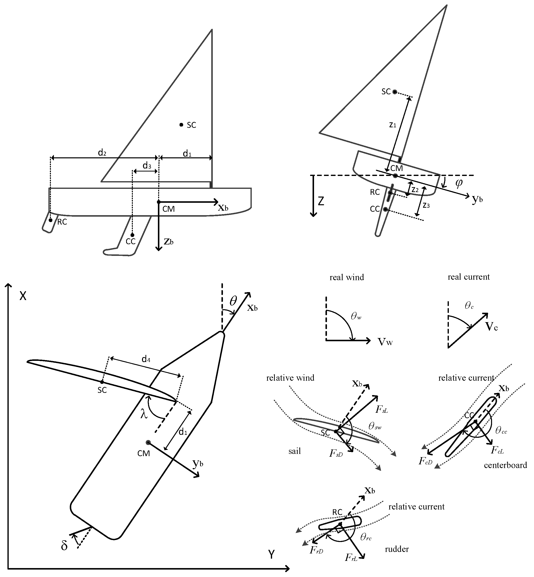
Jmse 09 01420 g001
Figure 2. The control architecture of the sailboat. It includes the sailboat system on the right side, the course control system on the upper side, and the speed controller on the lower side.
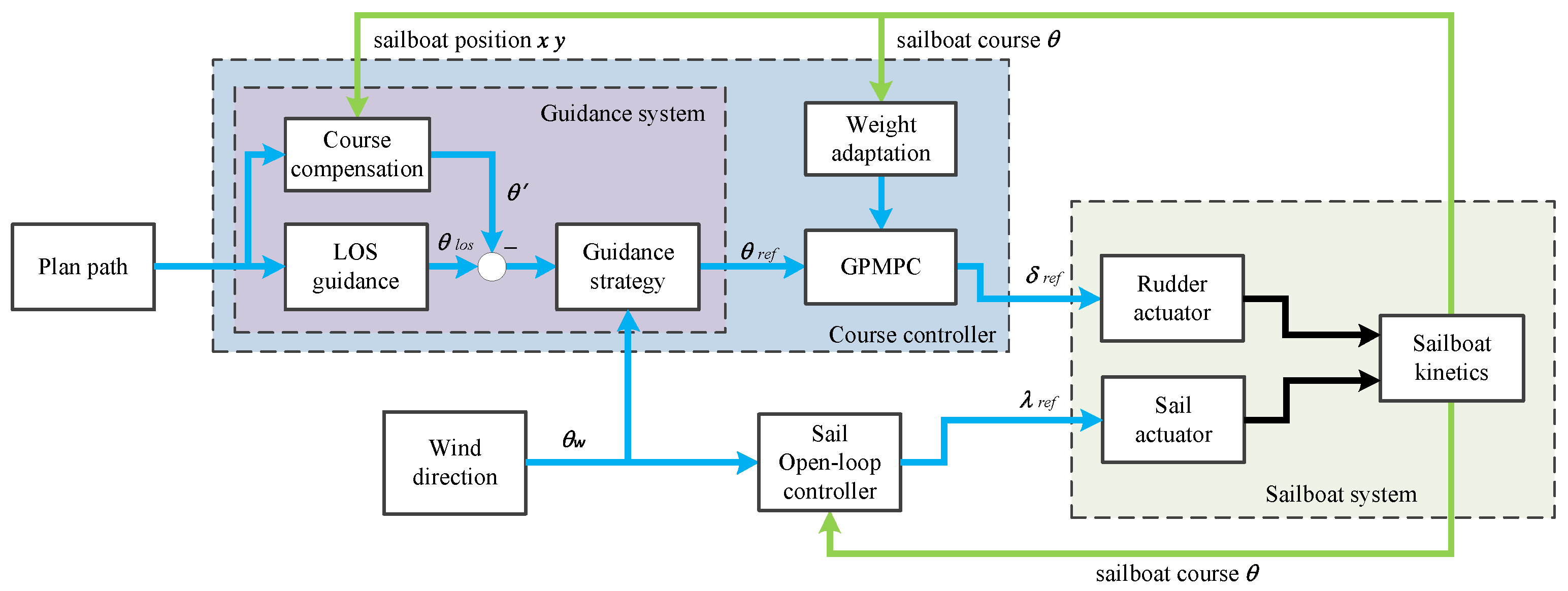
Jmse 09 01420 g002
Figure 3. The effect of weight adaptation term in the control process.
Jmse 09 01420 g003
Figure 4. The relationship between the windward angle and maximum forward speed of a sailboat.
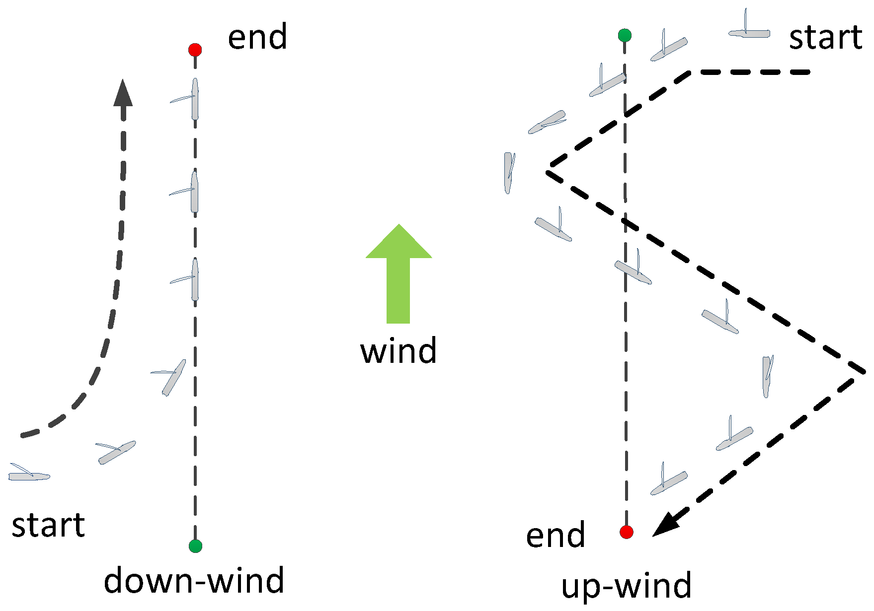
Jmse 09 01420 g004
Figure 5. Sailing in up-wind and down-wind.
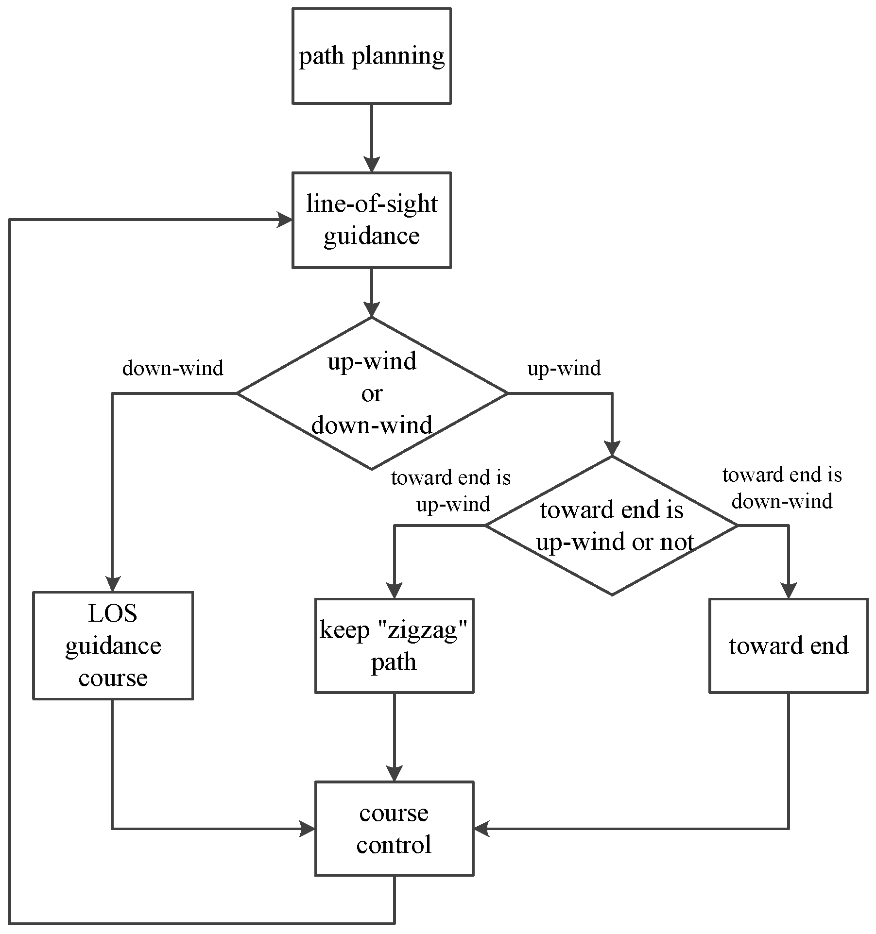
Jmse 09 01420 g005
Figure 6. Guidance strategy flow chart.
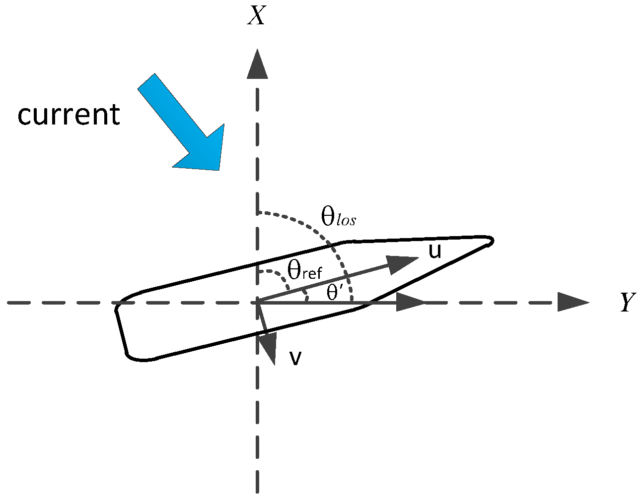
Jmse 09 01420 g006
Figure 7. Line-of-sight guidance.
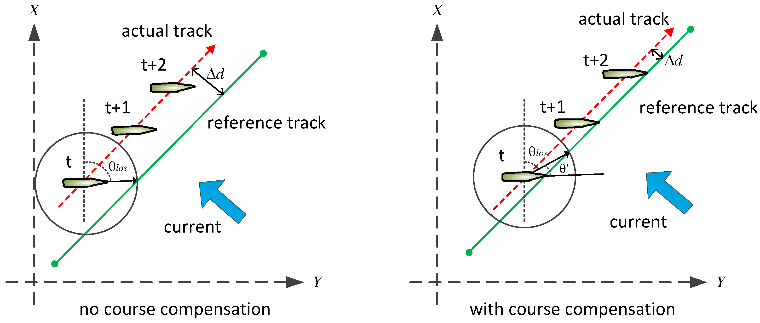
Jmse 09 01420 g007
Figure 8. Schematic diagram of heading deviation and the compensation.
Jmse 09 01420 g008
Figure 9. Effect of course compensation.
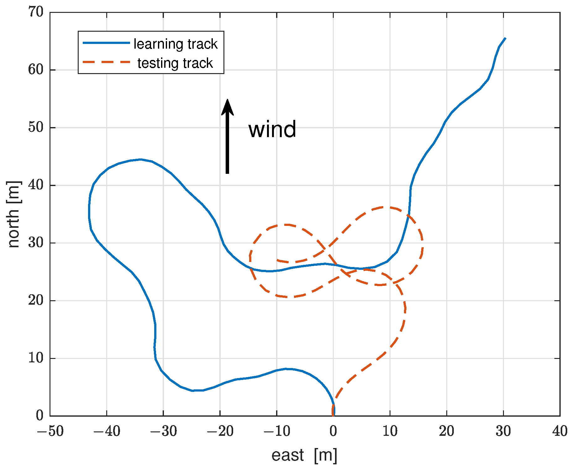
Jmse 09 01420 g009
Figure 10. The navigation data used for learning the Gaussian model. The navigation sampling data of the solid blue trajectory in the figure is used as the learning data of the Gaussian model. The navigation sampling data of the orange dashed line is used as test data to verify the accuracy of the Gaussian model.
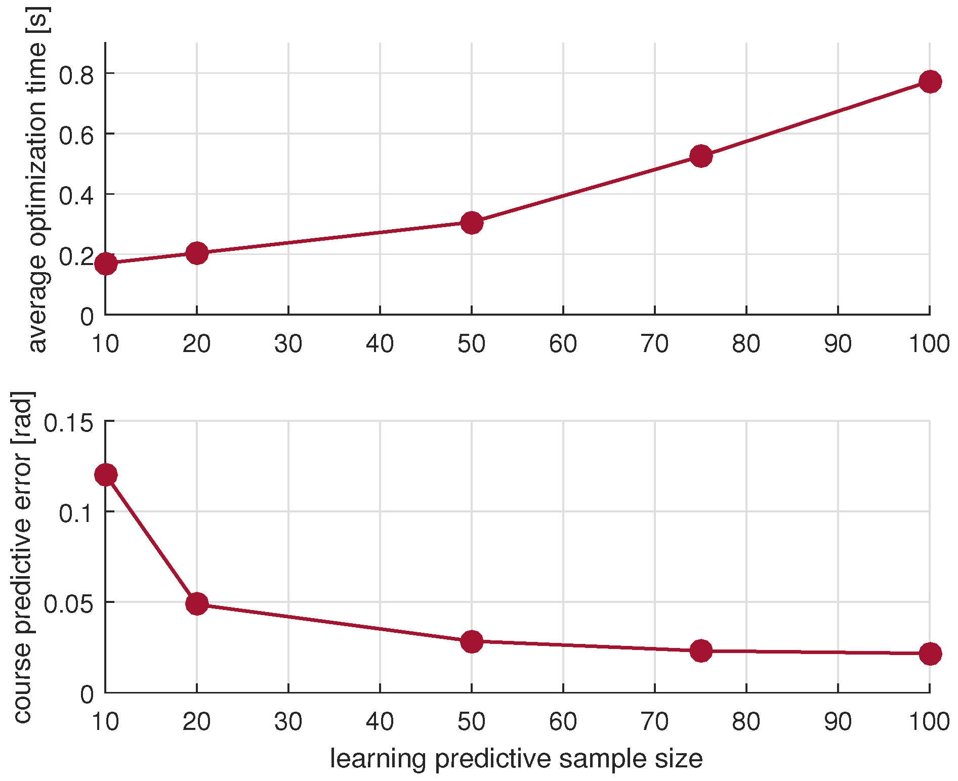
Jmse 09 01420 g010
Figure 11. The effect of learning sample size in Gaussian model on prediction accuracy and optimization time.
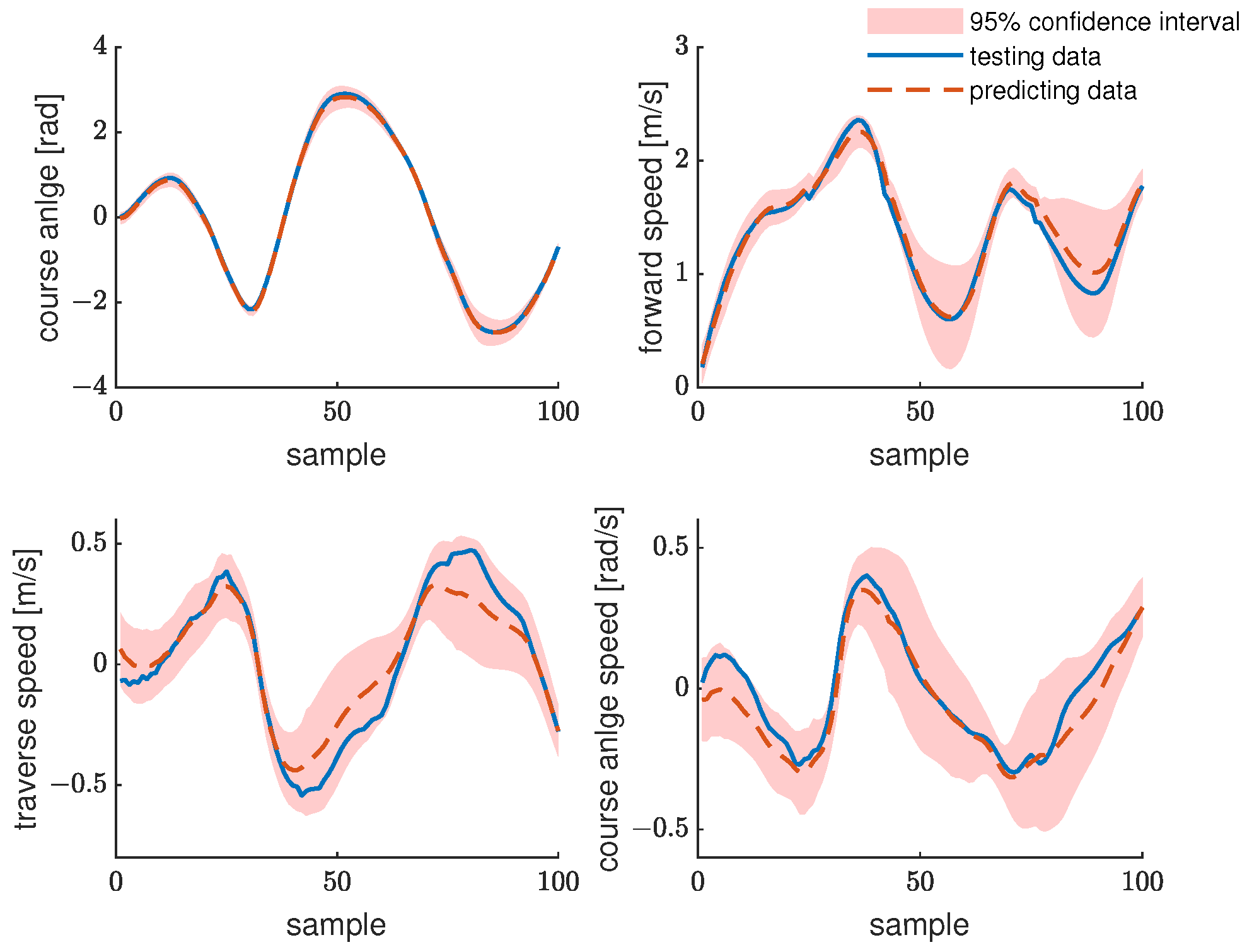
Jmse 09 01420 g011
Figure 12. Results of Gaussian model predictions. Prediction results for heading, forward speed, lateral speed, and yaw angle speed for the test data in the case of 50 learning samples. The solid blue line in the figure shows the actual data, the dashed orange line shows prediction results, and the red area shows the 95% confidence interval.
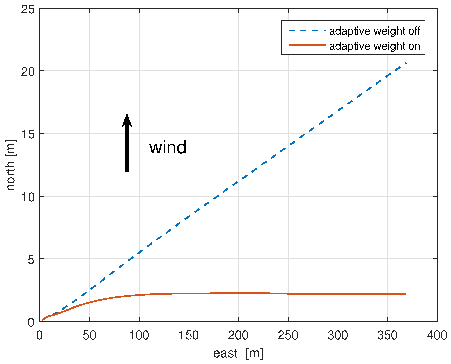
Jmse 09 01420 g012
Figure 13. Sailing trajectory with and without adaptive weight term. The blue dashed line in the figure is the trajectory without adaptive weight term, and the solid orange line is the trajectory with adaptive weight term, when keeping a 90 + 1.5 degrees course in calm water.
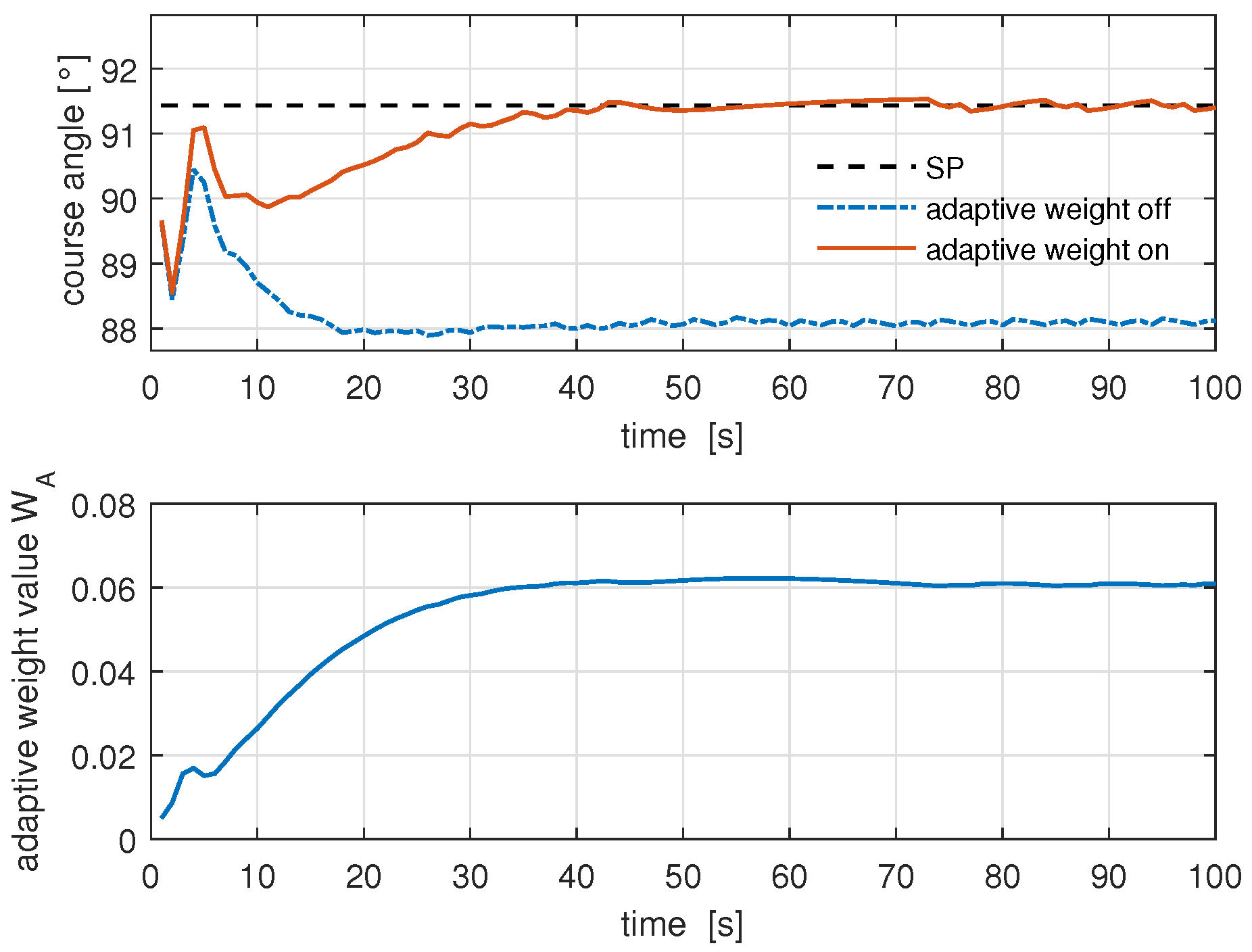
Jmse 09 01420 g013
Figure 14. Course tracking data with and without adaptive weight term. The top graph shows the change of heading during the course of navigation. The SP (Set Point) is heading control input. The solid orange line shows the change of heading with adaptive weight, and the dashed blue line shows the change of heading without adaptive weight. The lower graph shows the trend of the adaptive weight value W A during the course of the navigation.
Jmse 09 01420 g014
Figure 15. 
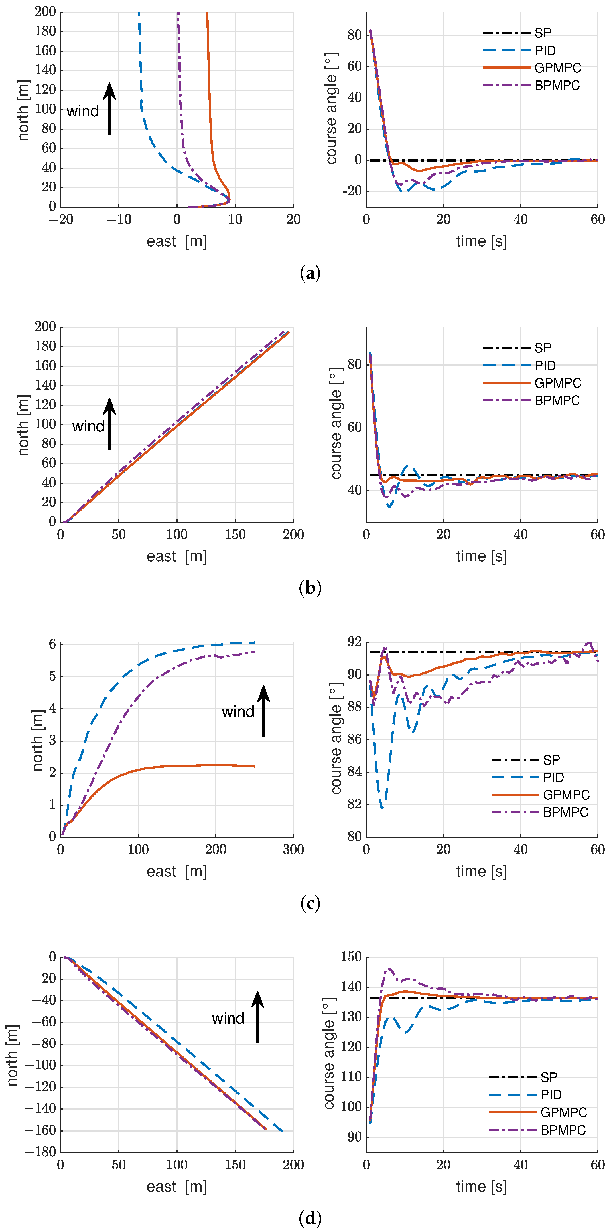
The sailing trajectory (left) and course angle curve (right) in different heading changes. The black dotted line is Set Point (SP), the blue dashed line is the PID control effect, the purple dotted line is the BPMPC control effect, and the orange solid line is the GPMPC control effect. (a) The course angle from 90 degrees to 0 degrees; (b) the course angle from 90 degrees to 45 degrees; (c) the course angle from 90 degrees to 90 + 1.5 degrees; and (d) the course angle from 90 degrees to 135 degrees.
Jmse 09 01420 g015
Figure 16. 
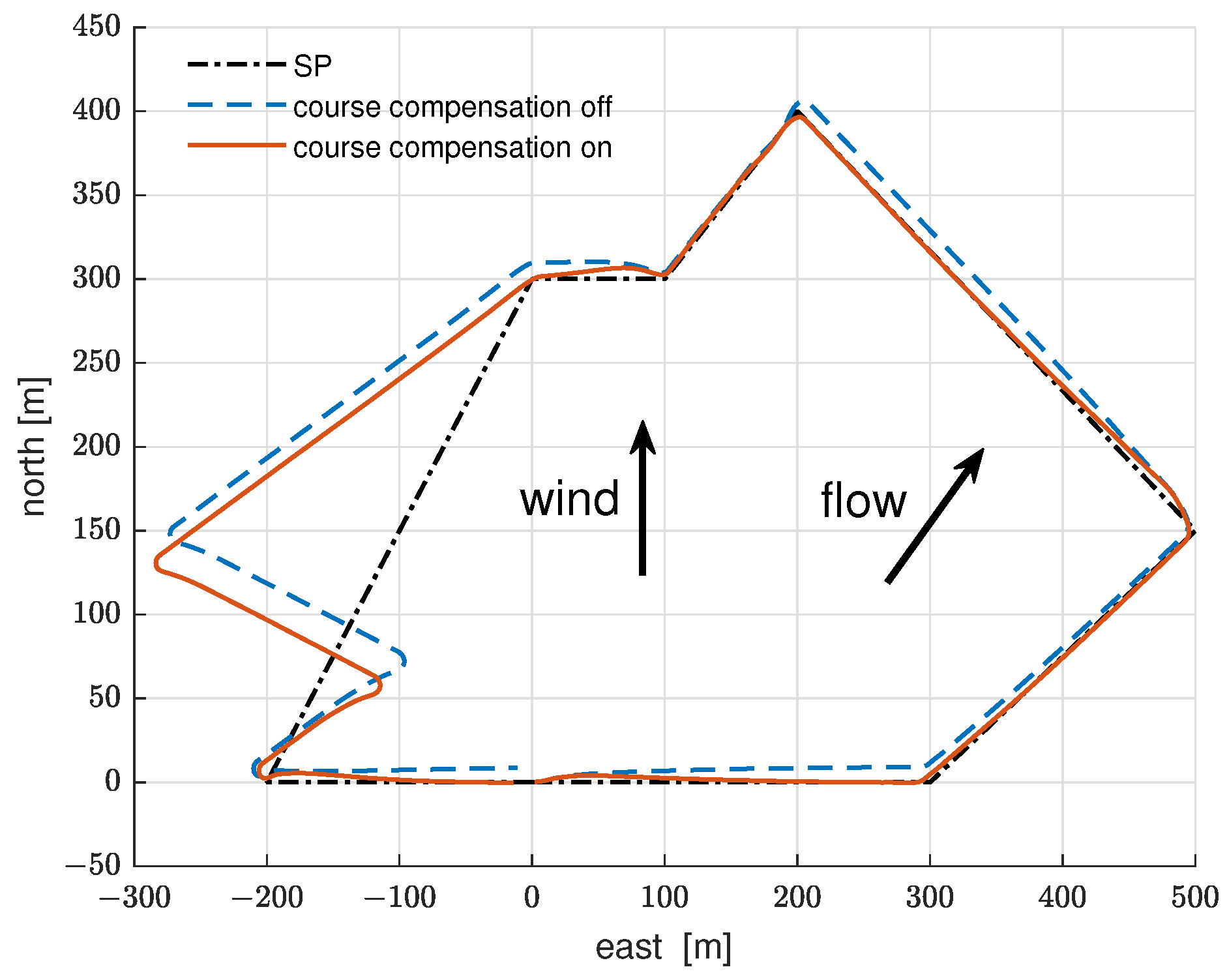
The sailing trajectory of LOS with and without heading compensation when there is current interference. The trajectory of waypoints in Table 3 with wind direction at 0 degree, wind speed at 5 m/s. The black dotted line SP is the reference trajectory, the blue dashed line is the case without heading compensation, and the orange solid line is the case with heading compensation.
Jmse 09 01420 g016
Figure 17. 
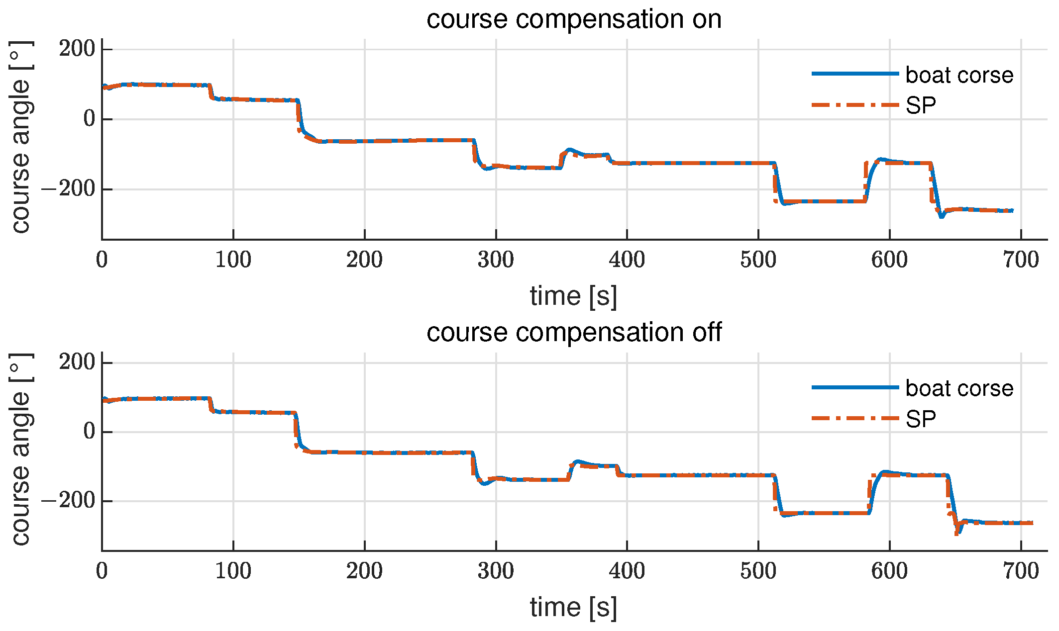
Course change response curve of LOS with and without heading compensation in the current environment. The solid blue line is the actual heading and the dotted orange line SP is the control input.
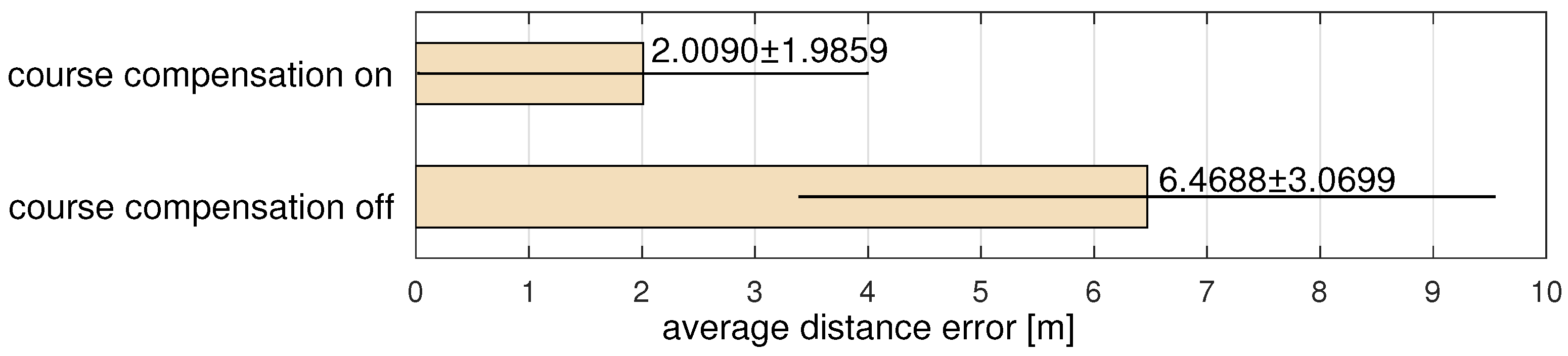
Jmse 09 01420 g017
Figure 18. The distance deviation from the reference trajectory. The mean and standard deviation of the distance deviation with and without heading compensation, for both control modes.
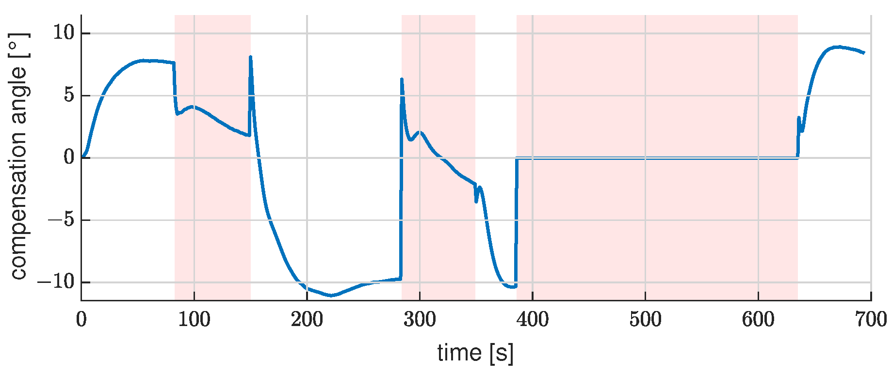
Jmse 09 01420 g018
Figure 19. Heading compensation amount. The amount of heading compensation for each course track during navigation, which is zero when sailing up-wind because there is no reference track.
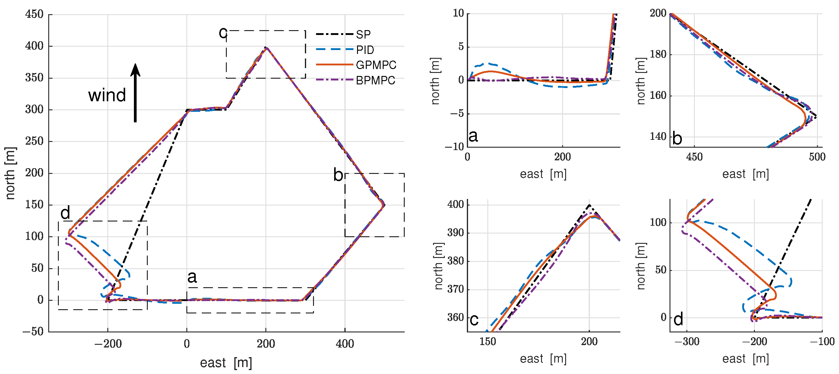
Jmse 09 01420 g019
Figure 20. The sailing trajectory under the calm water surface. The black dotted line in the figure is the reference trajectory, the blue dashed line is the PID control effect, the purple dotted line is the BPMPC control effect, and the orange solid line is the GPMPC control effect. The right side shows the zoomed-in view of the local trajectories in the four areas of (ad).
Jmse 09 01420 g020
Figure 21. Heading change under calm water. The top graph shows the response curve of heading change under PID control, the middle graph shows the response curve of heading change under BPMPC control, and the bottom graph shows the response curve of heading change under GPMPC control, the solid blue line is the actual heading and the dashed orange line is the target heading.
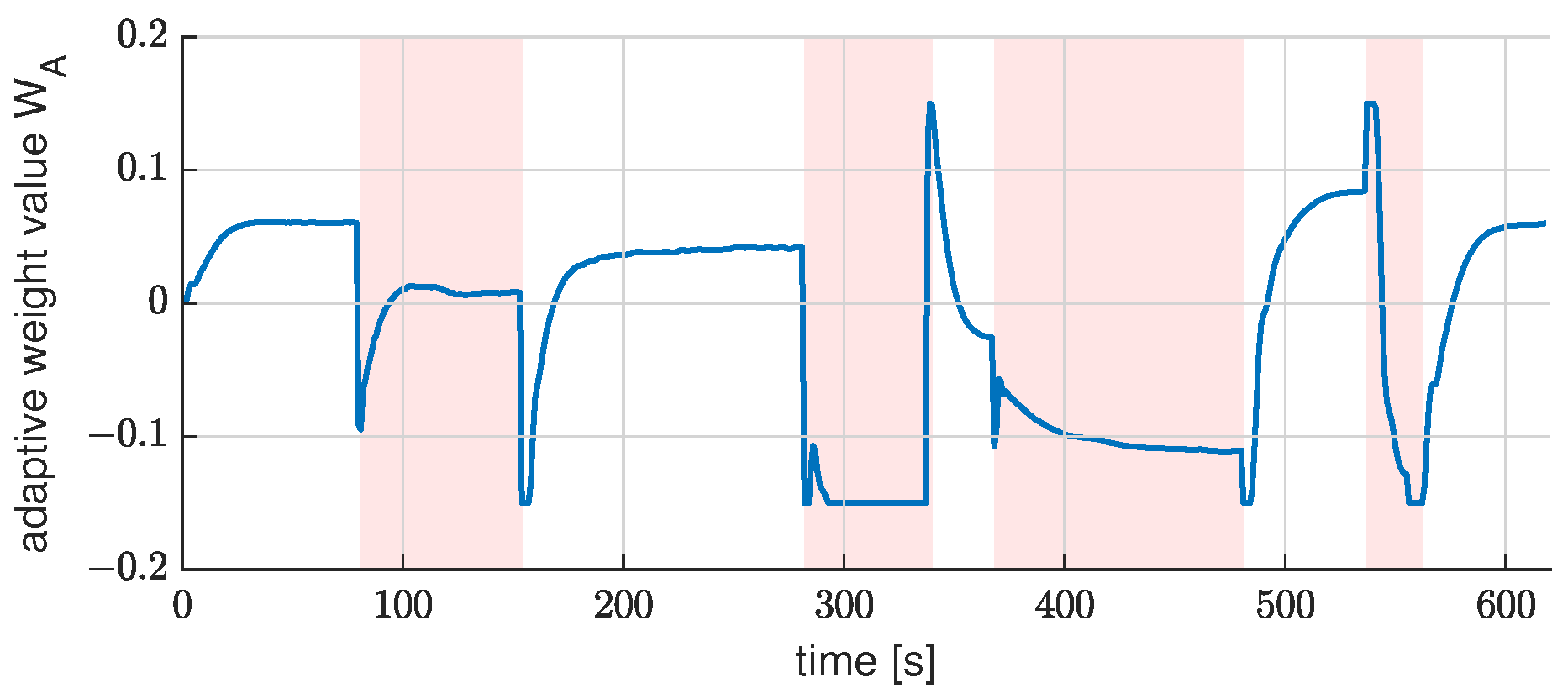
Jmse 09 01420 g021
Figure 22. The change in the adaptive weight value for each leg of the course during navigation.
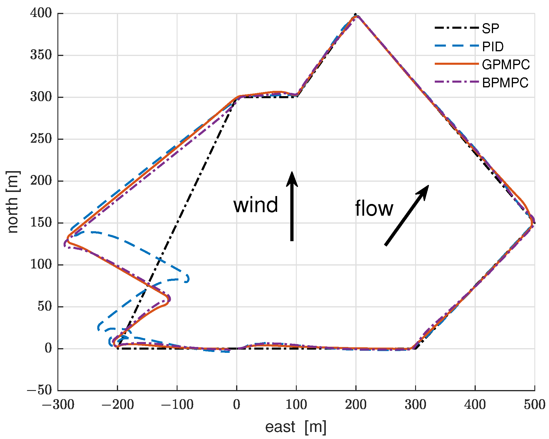
Jmse 09 01420 g022
Figure 23. Sailing trajectory with current disturbance. The black dotted line is the reference trajectory, the blue dashed line is the PID control, the purple dotted line is the BPMPC control effect, and the orange solid line is the GPMPC control.
Jmse 09 01420 g023
Figure 24. The response curve of heading change with and without course compensation for LOS with current disturbance. The top graph shows the PID control case, the middle graph shows the BPMPC control case, and the bottom graph shows the GPMPC control case. The solid blue line is the actual heading and the dashed orange line is the target heading.
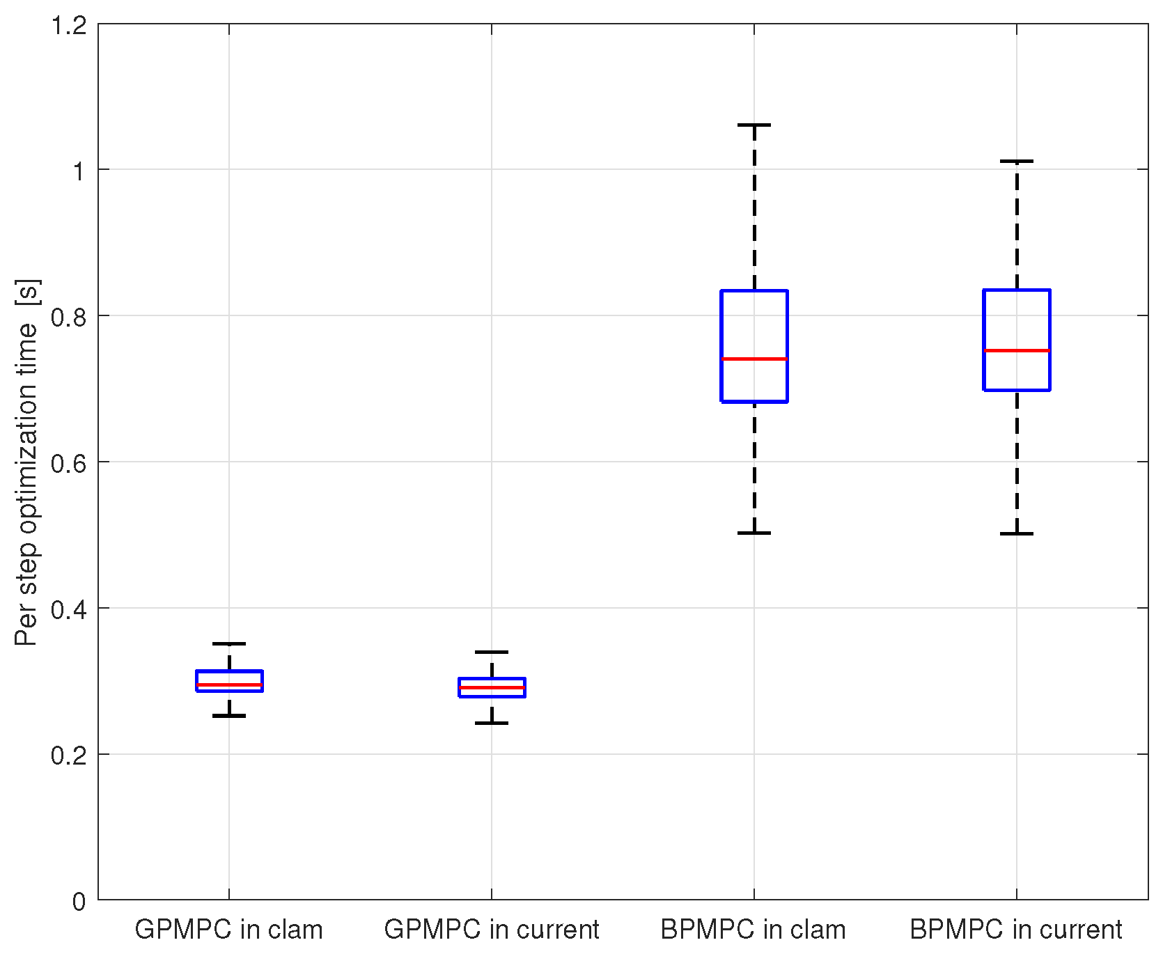
Jmse 09 01420 g024
Figure 25. Single step optimization time statistics of GPMPC and BPMPC under different conditions (box diagram).
Jmse 09 01420 g025
Table 1. Variable definitions.
VariableDescription
x Sailboat X-axis position
y Sailboat Y-axis position
φ Sailboat roll angle
θ Sailboat yaw angle
u Sailboat forward velocity
v Sailboat transverse velocity
r Sailboat roll velocity
w Sailboat yaw velocity
λ Sail angle
δ Rudder angle
X , Y , Z Geodetic coordinate
x b , y b , z b Sailboat hull coordinate
CMSailboat center of mass
SC, CC, RCForce center of sail/centerboard/rudder
F s L , F s D Lift force and drag force of sail
F c L , F c D Lift force and drag force of centerboard
F r L , F r D Lift force and drag force of rudder
θ w , θ c Absolute wind/current angle
V w , V c Absolute wind/current velocity
θ sw , θ cc , θ rc Relative angle between fluid and foil
δ r e f , λ r e f , θ r e f Reference input of rudder/sail/course
θ l o s Line of sight guidance heading
Table 2. Sailing physical parameters.
ParameterValue
Rigid body mass matrix M R B = M 0 0 0 0 M 0 0 0 0 I x x 0 0 0 0 I z z
Added mass matrix M A = 160 0 0 0 0 1267 0 399 0 0 1092 0 0 399 0 2447
Rigid body coriolis matrix C R B = 0 M w 0 0 M w 0 0 0 0 0 0 0 0 0 0 0
Added coriolis matrix C A = 0 0 0 1267 v r + 399 r 0 0 0 160 u r 0 0 0 0 1267 v r 399 r 160 u r 0 0
Mass M = 1600
x b -axis moment of inertia I x x = 3300
z b -axis moment of inertia I z z = 4600
Table 3. Planned waypoints.
Number12345678
x[m]0015040030030000
y[m]03005002001000−2000
Table 4. The control accuracy of heading deviation and vertical distance deviation.
Case ACase BCase CCase DCase ECase FCase G
RMS of Δ θ 0.24130.25720.20470.30210.20220.18470.1903
CEP95 of Δ θ 0.43830.29810.11780.71030.25460.17910.1960
RMS of Δ d 2.67031.78212.01183.70473.01282.82327.1267
CEP95 of Δ d 6.43673.19513.68898.93546.11715.18129.7369
Table 5. The dynamic response index of course tracking control.
Case ACase BCase CCase DCase ECase F
Maximum overshoot42.4%27.2%23.8%47.3%26.1%9.89%
Maximum adjustment time36 s16 s15 s42 s18 s17 s
Publisher’s Note: MDPI stays neutral with regard to jurisdictional claims in published maps and institutional affiliations.

