A Novel Improved Coupled Dynamic Solid Boundary Treatment for 2D Fluid Sloshing Simulation

Abstract

In order to achieve stable and accurate sloshing simulations with complex geometries using Smoothed Particle Hydrodynamic (SPH) method, a novel improved coupled dynamic solid boundary treatment (SBT) is proposed in this study. Comparing with the previous SBT algorithms, the new SBT algorithm not only can reduce numerical dissipation, but also can greatly improve the ability to prevent fluid particles penetration and to expand the application to model unidirectional deformable boundary. Besides the new SBT algorithm, a number of modified algorithms for correcting density field and position shifting are applied to the new SPH scheme for improving numerical stability and minimizing numerical dissipation in sloshing simulations. Numerical results for three sloshing cases in tanks with different geometries are investigated in this study. In the analysis of the wave elevation and the pressure on the tank, the SPH simulation with the new SBT algorithm shows a good agreement with the experiment and the simulations using the commercial code STAR-CCM+. Especially, the sloshing case in the tank with deformable bottom demonstrates the robustness of the new boundary method.

1. Introduction

Liquid sloshing is an important problem for the vessels with large liquid bulk cargo tanks, such as oil tank and liquefied natural gas (LNG) carriers. The motion of fluid in liquid tanks can be very violent and produce localized high pressure, which might endanger the vessel’s stability and tank structures. Sloshing in liquid tanks contains many complex nonlinear physical phenomena involving free surface flow, multiphase flow, wave breaking, splashing and reunion of fluids, etc. It is quite a challenge to accurately simulate the movement of fluid and the hydrodynamic load on the tank, especially for violent sloshing.

Smoothed Particle Hydrodynamic (SPH) is a meshless method, which is based on a Lagrangian formulation and has been successfully applied in many fields including biomedicine [1], astronomy [2], structural mechanics [3] and computational fluid dynamics [4]. Due to the Lagrangian nature, SPH has the advantage in simulating strongly nonlinear and discontinuous phenomena compared with traditional grid-based approaches. In recent years, many researchers have applied the SPH method to the simulation of strongly nonlinear free-surface flows, such as dam-breaking, multi-phase flow and liquid sloshing [5,6,7,8,9,10,11,12,13], because the SPH method does not need to track the free surface, which is usually a quite complicated problem for grid-based methods and numerical errors can easily be introduced [14,15].

However, there are still some challenges existing in weakly compressible SPH (WCSPH), such as boundary treatment and pressure oscillation [16]. Imposing boundary conditions in SPH is more complicated than grid-based methods because the foundation of SPH is the kernel-based interpolation theory. The consistency of particle field variables near boundaries cannot be guaranteed since the support domain of these particles is truncated by the boundaries. Numerical errors could be introduced by the kernel truncation if improperly treated [17]. There are many kinds of boundary methods in SPH proposed by researchers, such as repulsive functions method [18], boundary integrals method [19], mirror particles method [20] and fixed ghost particles method [21].

For SPH sloshing simulations, the fixed ghost particles method is probably the most popular boundary method because of the high computational efficiency and numerical accuracy. Ghost boundary particles representing the wall are pre-generated at the initial state and their spatial position is fixed with boundaries throughout the entire simulation. The physical quantities of boundary particles are computed by the boundary conditions and the properties of neighboring fluid particles. Adami et al. [22] proposed the fixed ghost particles method to model solid wall boundary. A force balance correction between the wall and the fluid particles is introduced to apply the pressure boundary condition on the boundary particles to prevent particle penetration. The sloshing simulation in a partially filled rotating rippled cylinder demonstrates that the method can handle complex moving boundaries interacting with violently moving free-surfaces. Shao et al. [23] and Liu et al. [24] presented an improved SPH method with Reynolds Averaged turbulence model for modelling liquid sloshing dynamics and proposed a coupled dynamic solid boundary treatment (SBT) algorithm based on the fixed ghost particles method. In the SBT algorithm, boundary particles are divided into repulsive particles and ghost particles. The repulsive particles produce a kernel-like, soft repulsive force to the approaching fluid particles near the boundary to prevent particle penetration. A reliable numerical approximation scheme for estimating the information of the two type boundary particles is introduced. With an improved approximation scheme with corrections of the density and kernel gradient, the SPH model has better accuracy with smoother pressure field. Numerical results including flow pattern, pressure field and pressure load on solid walls agree well with experimental results, and pressure oscillations are reduced significantly. Chen et al. [16] investigated the pressure on the solid wall in 2D sloshing for forced rolling motion using SPH method with the coupled dynamic SBT algorithm. The repulsive force formulation of the repulsive particles is improved and a great improvement in the pressure field near the solid boundaries is achieved. Besides, several improved correction algorithms, such as density re-initialization and a new boundary pressure measurement, are applied to the SPH sloshing simulation. The numerical pressure value of specified points on solid walls is more accurate and has a better agreement with the experimental results. In addition, Cao et al. [25] investigated the accuracy and stability of several kernel functions and applied the fixed ghost particle method to sloshing simulations in 2D and 3D tanks with or without a baffle. In order to achieve stable and accurate simulations of long duration sloshing with low fill ratios, Green and Peiró [26] combined the fixed ghost particle boundary method with a corrected $\delta$-SPH scheme to improve the stability with minimal energy dissipation. The numerical results of these simulations show the ability and accuracy of the method for simulations of prolonged durations.

It is obvious that these fixed ghost particles methods have many advantages, such as computational simplicity, high numerical stability and accuracy, and great flexibility in application of complex geometries. However, some intrinsic drawbacks of the fixed ghost particles method still exist. For violent sloshing problems, fluid particles might penetrate and cross the wall, especially when a coarse distribution of boundary particles is used. In addition, these boundary methods cannot be applied to model deformable boundaries because, fluid particles could penetrate the wall when the distance between boundary particles increases with the deformable boundaries, which could result in numerical instability and greatly limit its application to fluid-structure interactions.

In the present study, an improved coupled dynamic SBT algorithm is proposed for numerical simulation of liquid sloshing. The new boundary method in this study can not only be used to model rigid boundaries, but also unidirectional deformable boundaries. Besides the new SBT algorithm, a number of modified algorithms for correcting the density field and position shifting are applied to the SPH scheme to guarantee the numerical stability and accuracy over prolonged durations. The effectiveness of the SPH scheme with the new SBT algorithm is validated for several cases of liquid sloshing, including sloshing cases with vertical unidirectional deformable boundaries.

2. The SPH Scheme

The governing equations following the Navier–Stokes equations can be expressed in Lagrangian form as:

$$\{\begin{array}{c}\frac{d\rho }{dt}=-\rho \overrightarrow{\nabla }\cdot \overrightarrow{v}\\ \frac{d\overrightarrow{v}}{dt}=-\frac{1}{\rho }\overrightarrow{\nabla }P+\overrightarrow{F}+\overrightarrow{\mathsf{\Theta }}\end{array}$$

(1)

where $\rho ,\overrightarrow{v},P,\overrightarrow{F}$ and $\overrightarrow{\mathsf{\Theta }}$ denote the density, the velocity, the pressure, the external body force and the diffusion terms, respectively.

Based on the assumption that the fluid is weakly compressible, the continuity and momentum equations are coupled by means of the Tait’s equation of state [27]:

$$P=\frac{{\rho }_0{c}_s^2}{\gamma }\left[{\left(\frac{\rho }{{\rho }_0}\right)}^{\gamma }-1\right]$$

(2)

where ${\rho }_0$ is the nominal density of the fluid (1000 ${\mathrm{kg}/\mathrm{m}}^3$ for water), $c_s$ is the numerical sound speed which is set to a value more than 10 times the maximum speed of the fluid field; $\gamma$ is a parameter set to 7 for water to ensure small changes in density lead to large changes in pressure ensuring weak compressibility. The fluid pressure $P$ is set to non-negative for the numerical stability of SPH scheme.

In this study, the improved Gaussian kernel is adopted here. Compared with other kernels, the improved Gaussian kernel not only has a better numerical accuracy and stability, but also has the merits of computational simplicity and efficiency, and the kernel function is not sensitive to the disordered particle distribution [25]:

$$W\left(\overrightarrow{r},h\right)=\{\begin{array}{cc}{a}_d\left(e^{-q^2}-C\right)& q\le 3\\ 0& q>3\end{array}$$

(3)

where $W$ is the kernel function defined over the support domain for 2D simulations, $\overrightarrow{r}\left(x,z\right)$ the position vector, and $h$ the smoothing length, $q=\frac{\left|\overrightarrow{r}-{\overrightarrow{r}}^{\prime }\right|}{h}$, $a_d=\frac{1}{\pi h^2\left(1-10e^{-9}\right)}$,$C=e^{-9}$.

According to the kernel approximation and particle approximation of the SPH methodology, the continuity and momentum equations (Equation (1)) can be expressed in a discrete form:

$$\{\begin{array}{c}\frac{d{\rho }_i}{dt}={\displaystyle \sum _j{m}_j\left({\overrightarrow{v}}_i-{\overrightarrow{v}}_j\right)}\cdot \overrightarrow{\nabla }{W}_{ij}\\ \frac{d{\overrightarrow{v}}_i}{dt}=-{\displaystyle \sum _j{m}_j\left(\frac{P_i}{{\rho }_i^2}+\frac{P_j}{{\rho }_j^2}+{\mathsf{\Pi }}_{ij}\right)}\cdot \overrightarrow{\nabla }{W}_{ij}+\overrightarrow{F}\end{array}$$

(4)

where the subscript $i$ and $j$ denote the particle of concern and the neighboring particle in the support domain of the concerned particle $i$ respectively; $m_j$ and ${\rho }_j$ represent the mass and the density of the particle $j$ respectively; and ${\mathsf{\Pi }}_{ij}$ is the viscosity term. In this study, the artificial viscosity is applied to the momentum equation [28], which takes the form:

$${\mathsf{\Pi }}_{ij}=\{\begin{array}{cc}-\frac{\alpha {\overline{c}}_{ij}{\mu }_{ij}}{{\overline{\rho }}_{ij}}& {\overrightarrow{v}}_{ij}{\overrightarrow{r}}_{ij}<0\\ 0& {\overrightarrow{v}}_{ij}{\overrightarrow{r}}_{ij}>0\end{array}$$

(5)

where ${\overrightarrow{r}}_{ij}={\overrightarrow{r}}_i-{\overrightarrow{r}}_j$, ${\overrightarrow{v}}_{ij}={\overrightarrow{v}}_i-{\overrightarrow{v}}_j$, ${\mu }_{ij}=\frac{h{\overrightarrow{v}}_{ij}{\overrightarrow{r}}_{ij}}{{\left|{\overrightarrow{r}}_{ij}\right|}^2+0.01h^2}$, ${\overline{c}}_{ij}$ and ${\overline{\rho }}_{ij}$ are the average values of the numerical sound velocities and densities of particles $i$ and $j$, and $\alpha$ is a tuning parameter determined according to the characteristics of the specific problem of concern. It is obvious that the artificial viscosity term can provide a repulsive force when particles approach each other, which can prevent particles clump and improve numerical stability. Besides, density re-initialization is another effective way to smooth the density and pressure field. In this study, the first order Moving Least Squares (MLS) method is applied to re-initialize the density field of fluid particles [29]. The above SPH scheme mainly refers to the literature [16].

Numerical dissipation is much severer in sloshing simulations with deformable boundaries than those without, because deformable boundary, which the distance between boundary particles is varying, can intensify the particles clumping. A position shifting algorithm towards fluid particles is used in this study for preventing particles clump and improving particles distribution during the sloshing simulation [30,31]. The displacement correction vector $\delta {\overrightarrow{r}}_i$ of the particle shifting is calculated by the Fick’s law,

$$\delta {\overrightarrow{r}}_i=-D\nabla C_i$$

(6)

where $\nabla C_i=={\displaystyle \sum _j\frac{m_j}{{\rho }_j}\nabla w_{ij}}$ is the gradient of particle concentration, and $D$ is a diffusion coefficient. In this study, the diffusion coefficient is:

$$D=-A_{s}h\Vert {\overrightarrow{v}}_i\Vert \Delta t$$

(7)

where $A_s$ is the particle shifting coefficient which is a dimensionless parameter set by the characteristics of the specific problem, $\Vert {\overrightarrow{v}}_i\Vert$ is the velocity magnitude of Particle $i$, and $\Delta t$ is the time step. In this study, the particle shifting correction algorithm only is applied in these sloshing simulations with deformable boundaries. The particle shifting algorithm can greatly improve the numerical accuracy and stability, and reduce numerical dissipation for sloshing simulation with deformable boundaries.

The predictor-corrector scheme is adopted in this study for the time integration, and the fixed time step used in this study satisfies the Courant condition [32]. Besides, in the sloshing simulations, an initial time smoothing function $\lambda$ is applied to smooth the tank’s motion and the update of boundary particles’ physical quantities at the initial time,

$$\lambda =\{\begin{array}{cc}0.5\sin \left[\left(\frac{t}{t_{initial}}-0.5\right)\pi \right]+0.5,& t<t_{initial}\\ 1.0,& t\ge t_{initial}\end{array}$$

(8)

where $t_{initial}=1.0$ s.

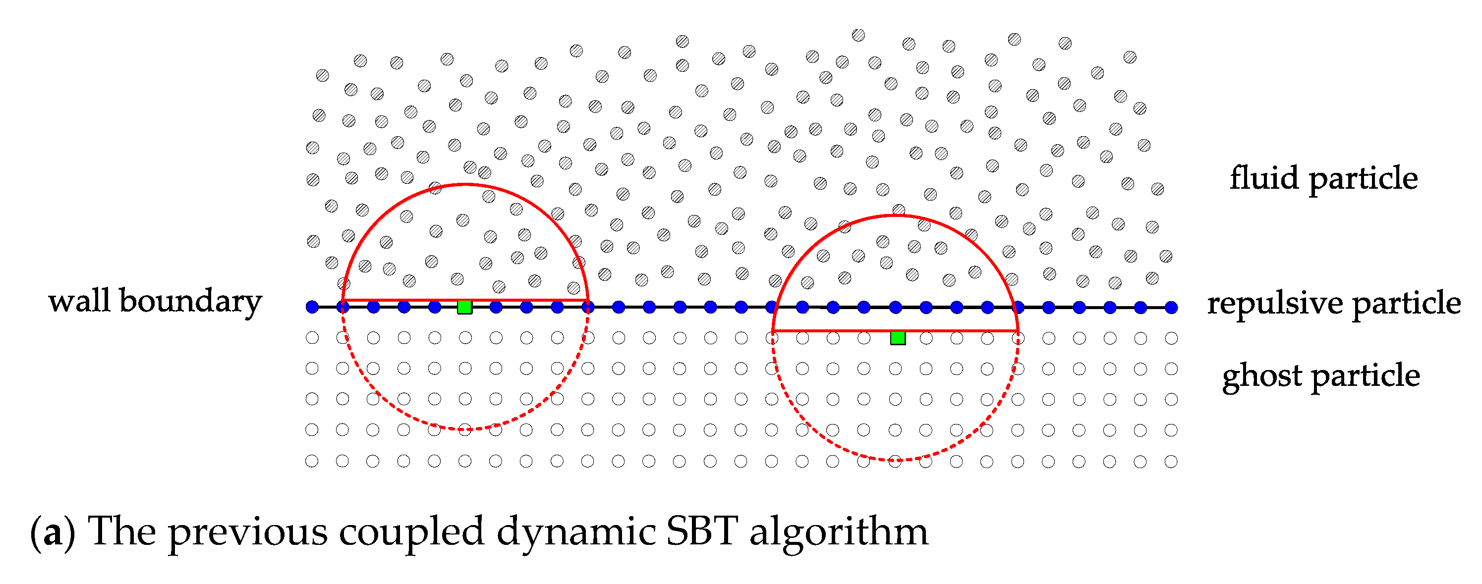
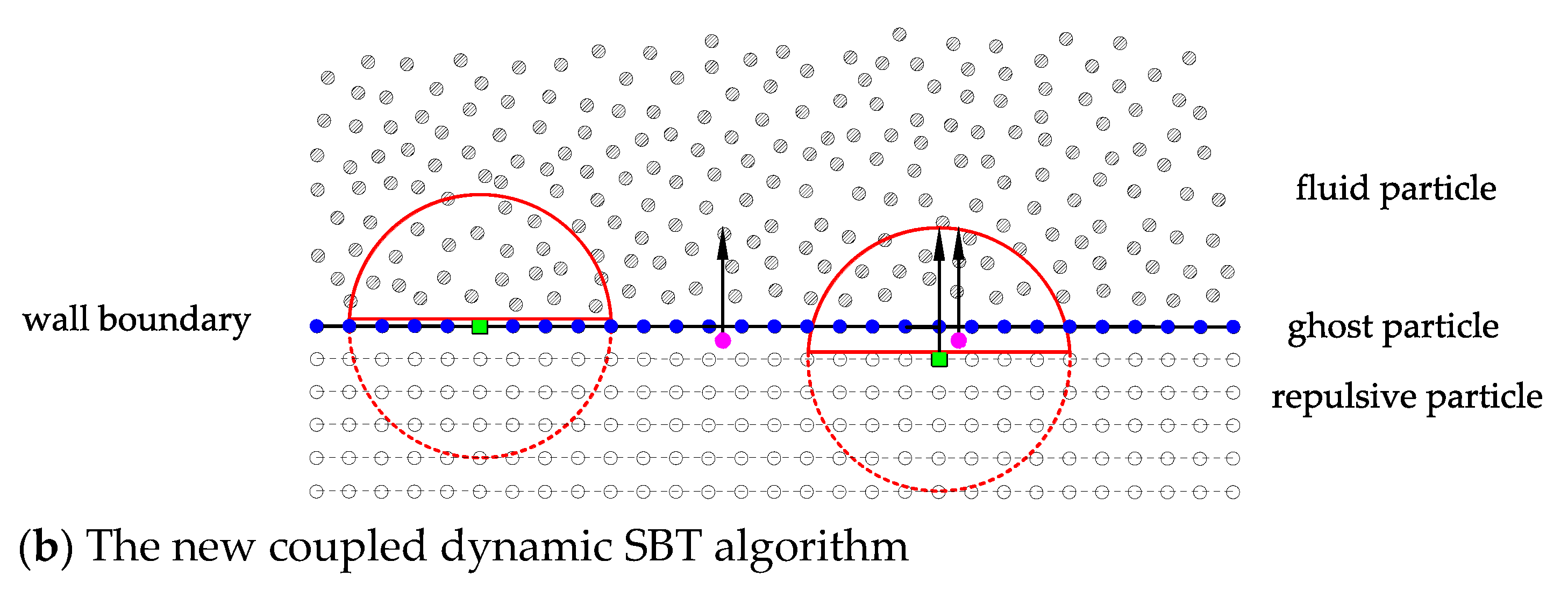
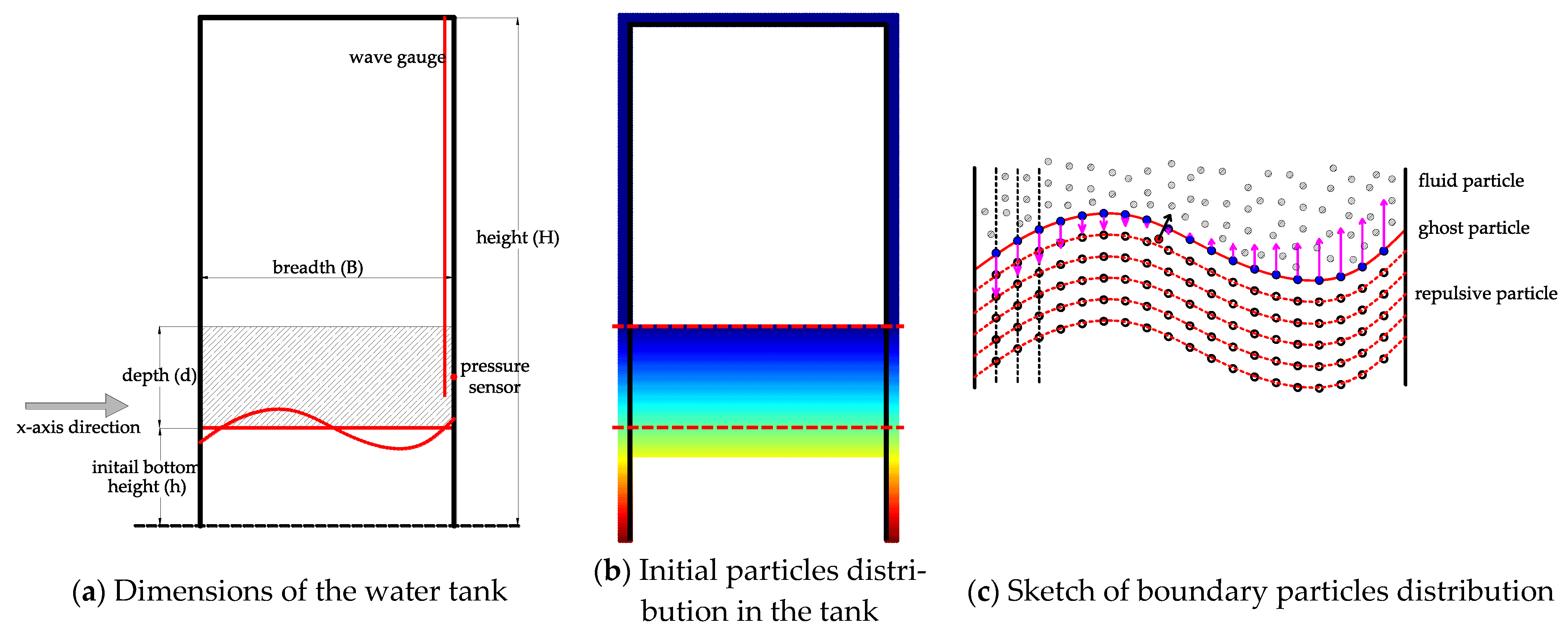
3. Wall Boundary Conditions Methodology

Because of the Lagrangian nature and the kernel-based interpolation theory of SPH, imposing the boundary condition is still a great challenge in SPH. A proper solid boundary treatment algorithm can greatly improve numerical accuracy and stability in SPH simulations.

In recent years, the coupled dynamic SBT algorithm, firstly developed by Liu et al. [24] and Shao et al. [23], is popular among SPH researchers. In the coupled dynamic SBT algorithm, boundary particles are divided into two types of particles: repulsive particles and ghost particles, as shown in Figure 1a. One inner layer of the repulsive particles is located right on the solid boundary, and several outer layers of the ghost particles are located outside the solid boundary area. Both repulsive particles and ghost particles possess physical quantities, such as mass pressure, density and velocity. Besides the same force as the ghost particles produce, repulsive particles will exert additional repulsive forces on the approaching fluid particles near the boundary. Chen et al. [16] reduced the acting distance of repulsive particles in reference [23] in order to avoid large initial errors and maintain the ability of preventing particles penetration in the meantime. The formulation of the repulsive forces in references [16,23] are given by,

$${\overrightarrow{F}}_{ij}=0.01{\overline{c}}_{ij}{}^2\cdot \chi \cdot f\left(\eta \right)\cdot \frac{{\overrightarrow{r}}_{ij}}{{\left|{\overrightarrow{r}}_{ij}\right|}^2}\cdot m_{fluid}$$

(9)

where

$$\{\begin{array}{ccc}\chi =1-\frac{\left|{\overrightarrow{r}}_{ij}\right|}{\Delta d},& 0<\left|{\overrightarrow{r}}_{ij}\right|<\Delta d& \left(\mathrm{in}\mathrm{reference}\left[23\right]\right)\\ \chi =1-\frac{\left|{\overrightarrow{r}}_{ij}\right|}{h},& 0<\left|{\overrightarrow{r}}_{ij}\right|<h& \left(\mathrm{in}\mathrm{reference}\left[16\right]\right)\end{array}$$

$$\{\begin{array}{cc}\eta =\frac{\left|{\overrightarrow{r}}_{ij}\right|}{0.75h}& \left(\mathrm{in}\mathrm{reference}\left[23\right]\right)\\ \eta =\frac{\left|{\overrightarrow{r}}_{ij}\right|}{0.5h}& \left(\mathrm{in}\mathrm{reference}\left[16\right]\right)\end{array}$$

$$f\left(\eta \right)=\{\begin{array}{cc}2/3,& \mathrm{for}0<\eta <2/3\\ \left(2\eta -1.5{\eta }^2\right),& \mathrm{for}2/3<\eta <1\\ 0.5{\left(2-\eta \right)}^2,& \mathrm{for}1<\eta <2\\ 0,& \mathrm{otherwise}\end{array}$$

where $\Delta d$ is the initial particle spacing.

However, it should be noted that both the SBT algorithms in references [16,23] cannot completely prevent the particles penetration. Fluid particle may still penetrate the solid boundary from the gap between boundary particles, especially in simulation of violent sloshing problems or with coarse boundary particles distributions. Besides, the inadequate ability of preventing particles penetration limits its application in modelling deformable boundary. In order to solve the problem, a new coupled dynamic SBT algorithm is proposed in this study. Different from the SBT algorithms in references [16,23], the position of the two type boundary particles is swapped with each other. The ghost particles, the inner layer of boundary particles, are located right on the solid boundary, and the outer layers of boundary particles located outside the solid boundary area are the repulsive particles. Besides, the formulation of the additional boundary repulsive forces can be rewritten as:

$$\begin{array}{cc}{\overrightarrow{F}}_{ij}=0.01{\overline{c}}_{ij}{}^2\cdot \chi \cdot f\left(\eta \right)\cdot \frac{\Delta d\cdot \overrightarrow{n}}{{\xi }^2+\kappa }\cdot m_{fluid}& \left({\overrightarrow{r}}_{ij}\cdot \overrightarrow{n}>0\right)\end{array}$$

(10)

where

$$\xi =\left|{\overrightarrow{r}}_{ij}\cdot \overrightarrow{n}\right|,\kappa =0.01\Delta d^2$$

$$\chi =\{\begin{array}{cc}1-\frac{\xi }{\Delta d},& \mathrm{for}0<\xi <\Delta d\\ 0,& \mathrm{otherwise}\end{array}$$

$$\eta =\frac{\left|{\overrightarrow{r}}_{ij}\right|}{0.5h}$$

$$f\left(\eta \right)=\{\begin{array}{cc}2/3,& \mathrm{for}0<\eta <2/3\\ \left(2\eta -1.5{\eta }^2\right),& \mathrm{for}2/3<\eta <1\\ 0.5{\left(2-\eta \right)}^2,& \mathrm{for}1<\eta <2\\ 0,& \mathrm{otherwise}\end{array}$$

where $i$ is the fluid particle, $\overrightarrow{n}$ is the unit normal vector at the position of repulsive particles $j$, pointing to the fluid domain, and $\xi$ is the distance between the fluid particle and the plane to which the repulsive particle belongs. It can be seen from the formulation of the additional boundary repulsive forces that the magnitude of the repulsive forces not only depends on the distance between the fluid particle and the repulsive particle, but also the distance between the fluid particle and the plane to which the repulsive particle belongs. The direction of the repulsive forces is the same as the normal vector of the boundary at the position of repulsive particles. In theory, the repulsive forces can almost completely prevent fluid particle penetration if $\kappa$ is small enough. But in simulation of violent sloshing problems, the magnitude of the repulsive forces could be very large and deteriorate the numerical stability if $\kappa$ is too small, or $\kappa =0$.

In the previous boundary methods, fluid particles that penetrate the solid boundary will be removed from the computation domain. In the new SBT algorithm of this study, the repulsive particles will exert repulsive forces to push the fluid particles back into the fluid domain when the fluid particles (red nodes in Figure 1b) penetrate the inner layer of ghost particles. In comparison with the previous SBT algorithms, this is an important improvement to reduce fluid particle penetration, especially for periodic sloshing simulations. The physical quantities for boundary particles are calculated by the MLS approximation, where the calculation method is the same as that in the previous SBT algorithms. In this study, the free-slip boundary condition is imposed on the fluid particles near the wall boundary, and the velocity of the boundary particles is directly made to equal to the solid boundary velocity [26].

The new SBT algorithm in this study optimizes the formulation of the additional boundary repulsive forces, and introduces the idea of forcing the fluid particles, penetrating the inner layer of boundary particles, back into the fluid domain.

4. Numerical Results

To verify the new SBT algorithm proposed in this study, a still water case and three typical sloshing test cases in liquid tanks are simulated using SPH. The tank’s geometries in the three violent sloshing cases are different, including a rectangular tank with uniform boundary particle distribution, a complex geometry tank with coarse boundary particle distribution and a tank with unidirectional deformable bottom. The numerical results are compared with experimental ones and also numerical results by other methods.

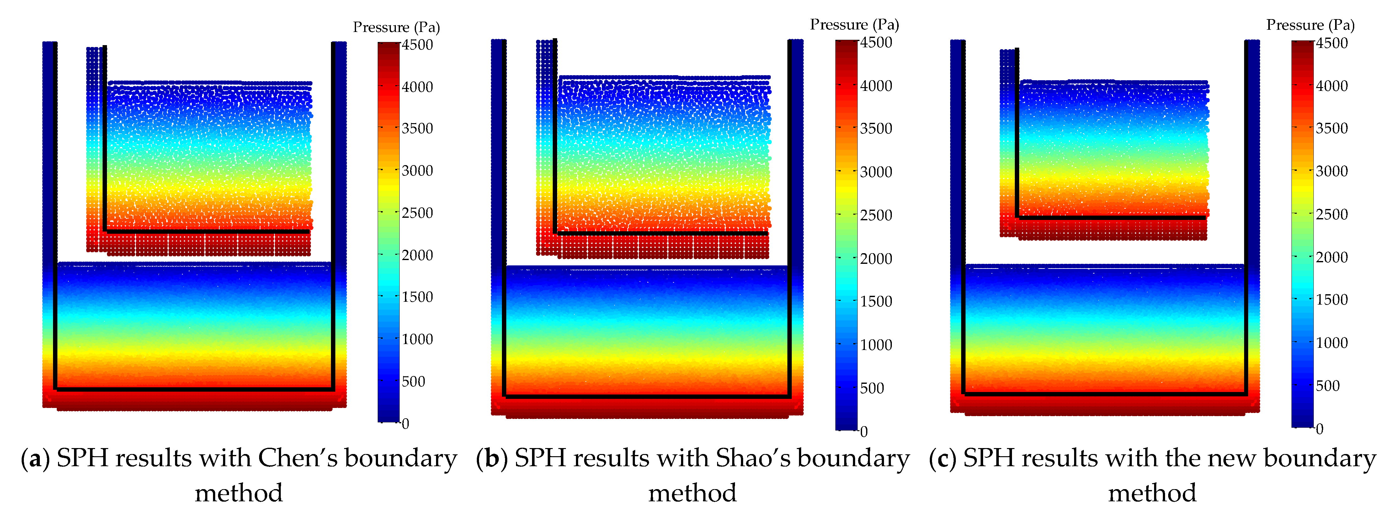
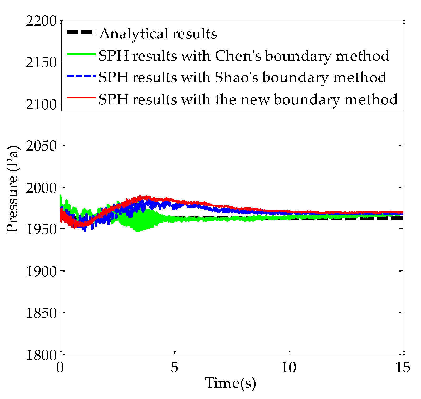
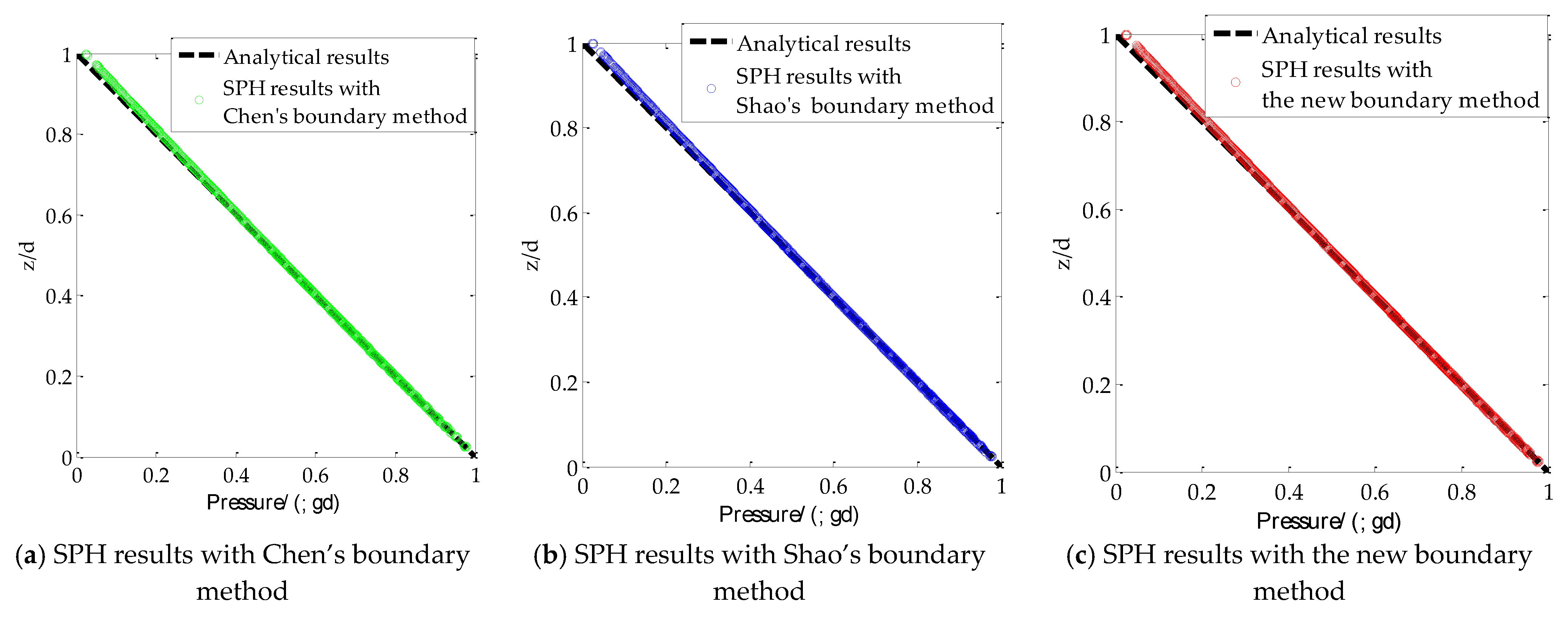
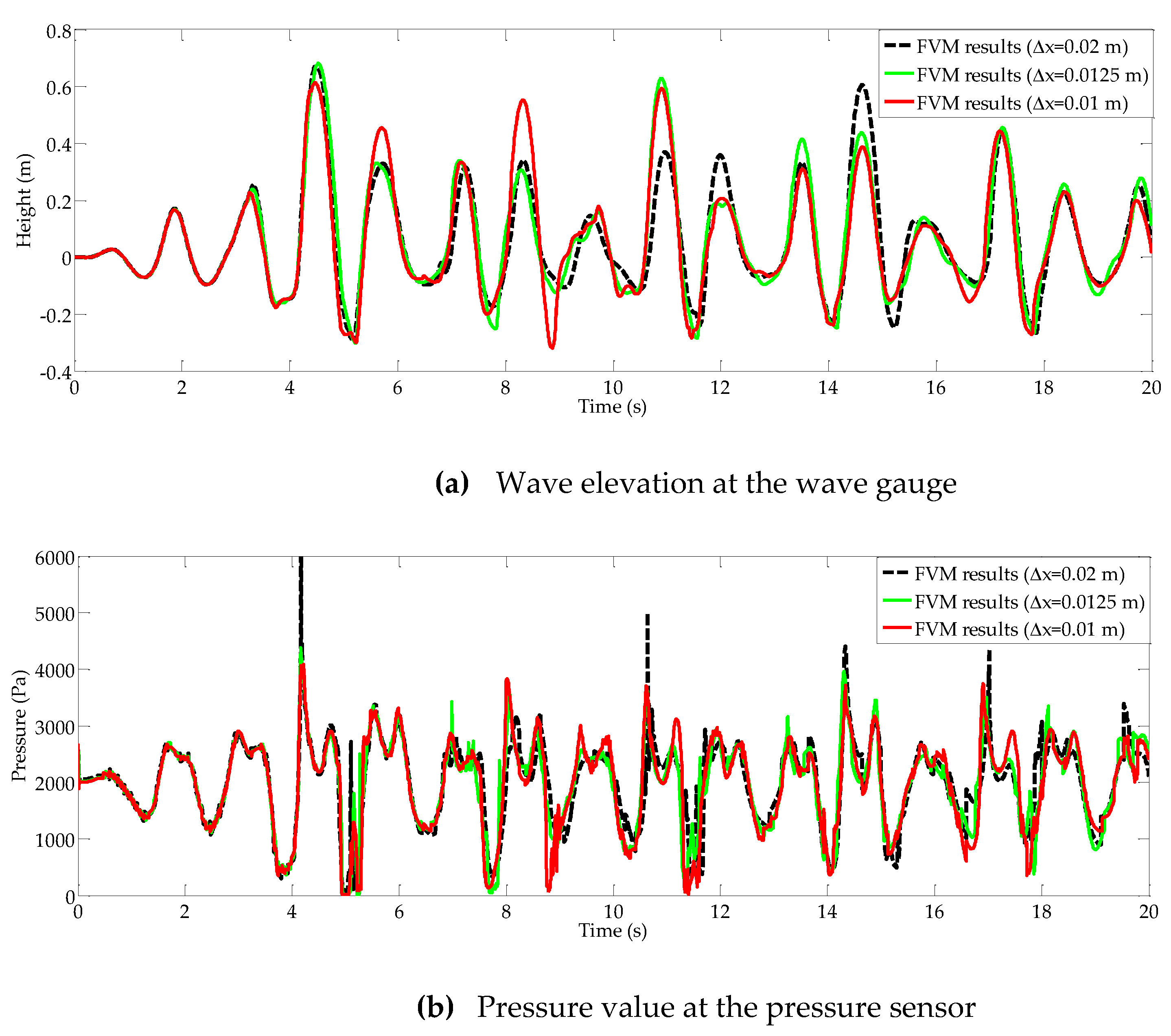
4.1. Still Water Case

In this section, a 2D still water case in a rectangular tank is simulated using SPH with different boundary methods. The breadth and height of the tank are 1.0 m and 1.0 m, and the initial water depth is $d=0.4\mathrm{m}$. A pressure probe point is placed 0.2 m below the initial free surface on the right wall. In the SPH simulations, the density of fluid particles is $\rho =1000{\mathrm{kg}/\mathrm{m}}^3$, and the numerical sound speed is $c_s=10\sqrt{gd}$. The artificial viscosity parameter $\alpha =0.02$ is used. The particle spacing is set to $\Delta x=0.01\mathrm{m}$, and the SPH time step is $5\times {10}^{-5}\mathrm{s}$. The MLS correction is applied to smooth the density field and approximate the physical quantities of boundary particles at every 5 time steps. The particle shifting algorithm is not applied to these SPH simulations of this section.

Figure 2 shows the pressure field and particle distribution at 15 s, which is a period of time after the initial disturbance and the pressure histories at the pressure sensor are very stable, as shown in Figure 3. All the pressure fields in Figure 2 are very smooth, and all the pressure values at the pressure sensor in Figure 3 are very close to the analytical results. Besides, the vertical distribution of pressure can also show the accuracy of the hydrostatic pressure distribution. Values of depth ($z/d$) against pressure $P/\left(\rho gd\right)$ for each fluid particle are shown in Figure 4. Although some slight discrepancies between the analytical values and the pressure values of the fluid particles near the free surface appear in Figure 4, all the SPH results obtained with different boundary methods are very accurate, generally.

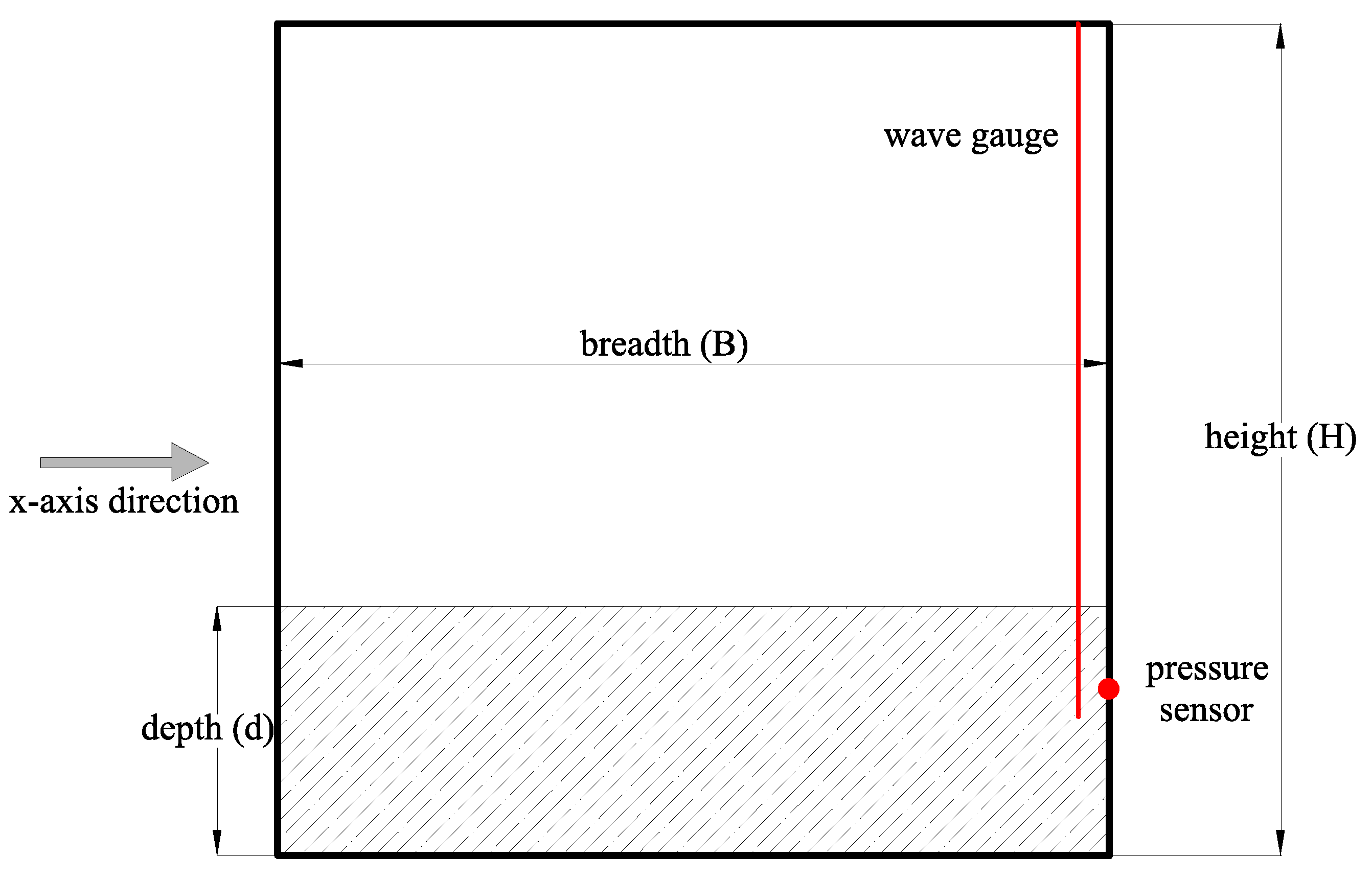
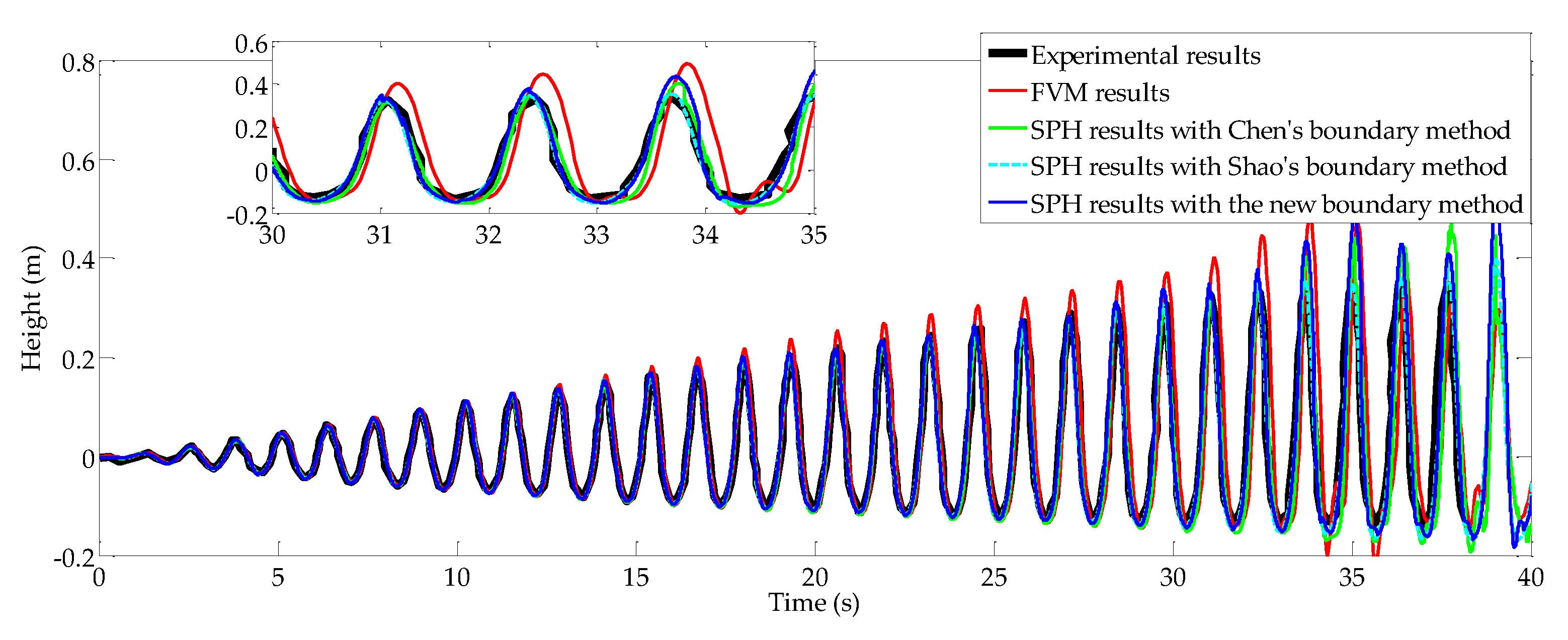
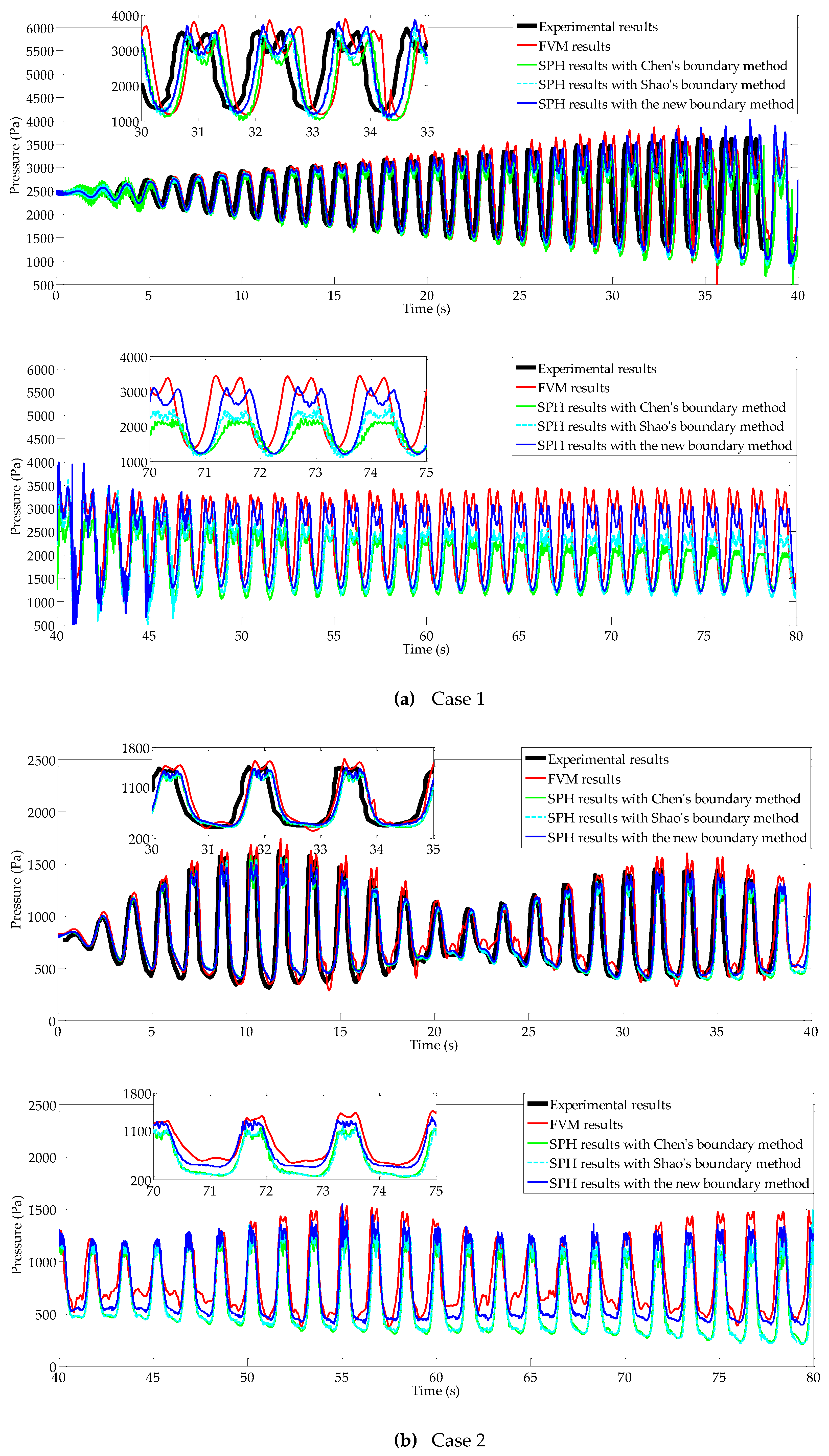
4.2. Sloshing in Rectangular Tank with Different Filling Ratios

In order to validate the accuracy and stability of the new SPH scheme, the experimental sloshing cases used by Pakozdi and Graczyk [33] are simulated using Finite Volume Method (FVM) and the SPH scheme with different SBT algorithms. More details about the experiments can be found in Cao et al. [34] and Pakozdi & Graczyk [33]. The dimensions of the 2D rectangular water tank are: breadth $B=1.0 \mathrm{m}$, height $H=1.0 \mathrm{m}$, and the water depth is $d$, as shown in Figure 5. A pressure probe point is placed 0.09 m above the bottom on the right wall. In addition, to visualize numerically the sloshing wave profile, a wave probe is placed 0.01 m from the right wall. The tank is subject to a sinusoidal translational excitation in the x-axis direction. In the SPH simulation, the excitation motion can be imposed in a moving frame of reference through a forcing term in continuum equation,

$$\overrightarrow{F}=\left(a\left(t\right),-g\right)$$

(11)

where $a\left(t\right)=\lambda A{\omega }^2\sin \left(\omega t\right)$ is the lateral acceleration, $\lambda$ is the initial time smoothing function, $A$ is the amplitude of displacement, and $\omega$ is the excitation frequency. The natural frequency of the sloshing system of a rectangular tank partially filled with water is ${\omega }_n^2=g\left(n\pi /B\right)\tanh \left(n\pi \left(d/B\right)\right)$. Hence, the first linear natural frequency is ${\omega }_1=\sqrt{g\left(\pi /B\right)\tanh \left(\pi \left(d/B\right)\right)}$. Two sloshing cases in the tank with different water depths are investigated by Pakozdi and Graczyk in the experiment. The frequencies and the amplitudes of the excitation motion of the tank corresponding to the sloshing cases are listed in

Table 1. Experimental parameters.

Cases	$\mathit{d}/\mathit{B}$	$\mathit{\omega }/{\mathit{\omega }}_1$	${\mathit{T}}_1,\mathbf{s}$	$\mathit{A}/\mathit{B}$
Case 1	0.337	0.985	1.2971	0.0040
Case 2	0.173	0.970	1.6576	0.0100

.

In the SPH simulation, the density of fluid particles is $\rho =1000{\mathrm{kg}/\mathrm{m}}^3$, and the numerical sound speed is $c_s=12\sqrt{gd}$. The artificial viscosity parameter $\alpha =0.02$ is used in this case. The particle spacing is set to $\Delta x=0.01\mathrm{m}$. Hence, the numbers of fluid particles these cases are 3332 and 1666 respectively, as listed in

Table 2. Numerical parameters in SPH simulation.

Cases	$\mathit{d}/\mathit{B}$	${\mathit{N}}_{\mathit{x}}\times {\mathit{N}}_{\mathit{z}}$
Case 1	0.340	$98\times 34$
Case 2	0.170	$98\times 17$

. There are some discrepancies in the water depths between the experiment and numerical simulations, but they are very small and negligible. The SPH time step is $5\times {10}^{-5}\mathrm{s}$. The MLS correction is applied to smooth the density field and approximate the physical quantities of boundary particles at every 5 time steps. The particle shifting algorithm is not applied to these SPH simulations of this section.

For the FVM simulations, which are based on the Euler two-phase separated flow model and computed using the commercial code STAR-CCM+, the computation domain is discretized into uniform grids with $\Delta x=0.01\mathrm{m}$, too. Due to the restrictions of the grid size, the numerical parameters are the same as those in the SPH simulation, as shown in Table 2. For all FVM simulations in this section, the time step is set to 0.001 s, which satisfies the Courant condition. The interface between water and air is captured with a volume of fluid (VOF) technique [14]. STAR-CCM+ is a reliable numerical tool, which has been widely used by many researchers for sloshing simulations [35,36,37]. The results of the FVM simulation are chosen as the benchmark value.

Figure 6 and Figure 7 show the comparison of the pressure and the wave elevation on the measuring probes from the numerical results and the experimental results for the two sloshing cases, which the experimental results only present in 38 s [34]. As seen in Figure 6 and Figure 7, all the numerical results of 0–40 s are in good agreement with the experiment in both the wave elevation and the pressure on the tank, and the SPH results with different boundary methods are very close to each other. However, for the numerical results of 40–80 s, the SPH results with the previous boundary methods show some obvious discrepancies with the FVM results and the SPH results with the new boundary method. It should be noted that the obvious numerical errors of the SPH results in Figure 6a at 38–42 s are caused by the splashing fluid particles, because the wave probe is easily disturbed by these splashing fluid particles.

As shown in the pressure histories of Figure 7, the numerical dissipation in the SPH simulations with the previous boundary methods is becoming severer as the simulation goes. In the previous coupled dynamic SBT algorithm of Shao et al. and Chen et al., one inner layer of the repulsive particles is arranged right on the solid boundary, and the repulsive force produced by the repulsive particles can improve the ability of preventing fluid particles penetration compared with the traditional fixed ghost particles method. On the other hand, however, the repulsive force can also produce severe numerical dissipation for long duration simulation. In the new coupled dynamic SBT algorithm of this study, the outer layers of boundary particles located outside the solid boundary area are the repulsive particles, and the repulsive particles only exert repulsive forces on the fluid particles which have crossed the inner layer of ghost particles. Thus, in the SPH simulations with the new boundary method, the pressure history is more stable throughout the entire simulation, and the downtrend of the pattern of the SPH results with the new SBT algorithm is smaller, as shown in Figure 7. The numerical dissipation of the SPH simulations with the new boundary method is very small, and the numerical error is approximately within 10% of the FVM results, as shown in Figure 7. However, the numerical error of the SPH results obtained with the previous boundary method can be more than 25% of FVM results, approximately.

For further investigating the numerical dissipation, three different values of the numerical sound speed $c_s$, namely $c_s=10\sqrt{gd}$, $c_s=12\sqrt{gd}$ and $c_s=13\sqrt{gd}$, are used in the SPH simulation with different SBT algorithms for the Sloshing Case 1. Figure 8 shows the comparison of the pressure histories obtained from the FVM simulation and the SPH simulations with different SBT algorithms. As shown in Figure 8, although there are some measurements proposed by Chen et al. [16] to avoid the large initial errors, there is still a drawback of the previous SBT algorithms, especially for these SPH simulations with a large value of $c_s$. However, due to the innovative arrangement of the repulsive particles, the SPH simulations with the new SBT algorithm not only have small numerical dissipation, but also have small initial errors. As shown in Figure 8c, the SPH results with $c_s=13\sqrt{gd}$ are very close to the FVM results, and the numerical dissipation is extremely small.

The numerical accuracy and stability of the new coupled dynamic SBT algorithm have been validated by these sloshing simulations in the rectangular tank. However, due to the simple geometry of the water tank and the uniform distribution of boundary particles, very few fluid particles can penetrate the solid wall and activate the repulsive forces of the repulsive particles. Thus, more violent sloshing cases with complex geometry need to be investigated.

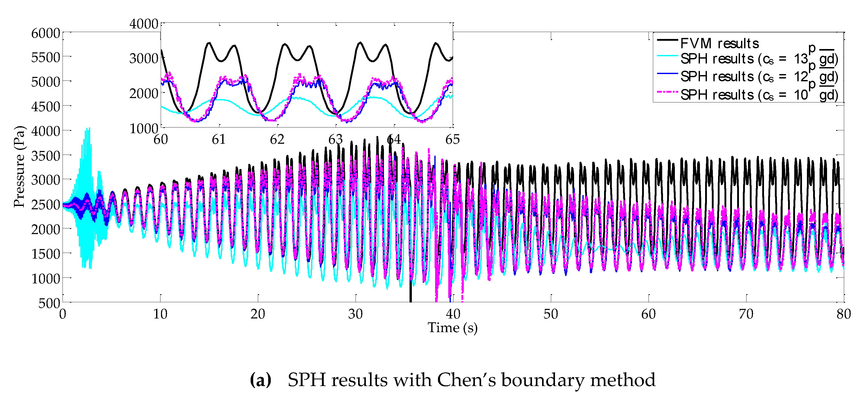
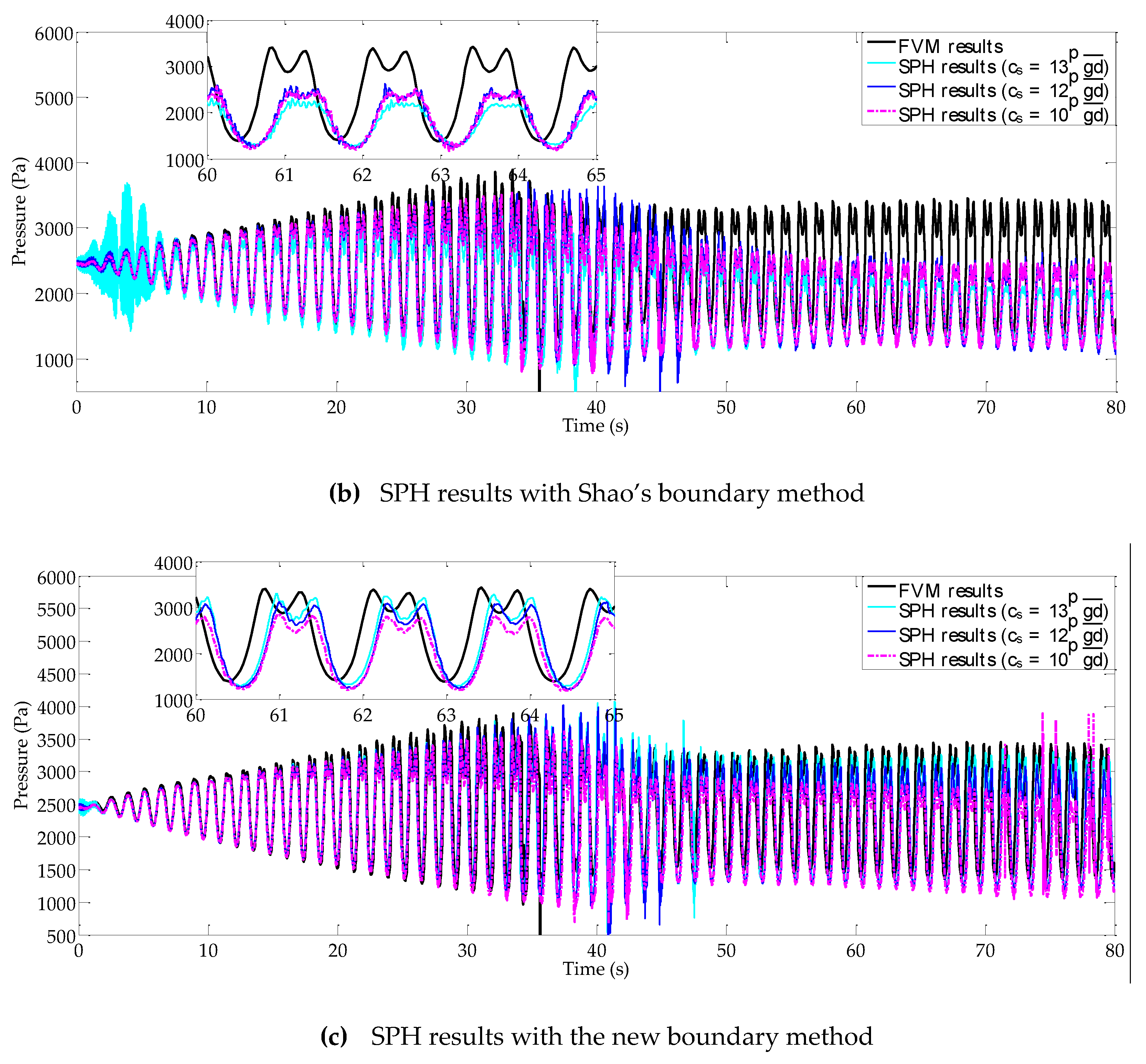
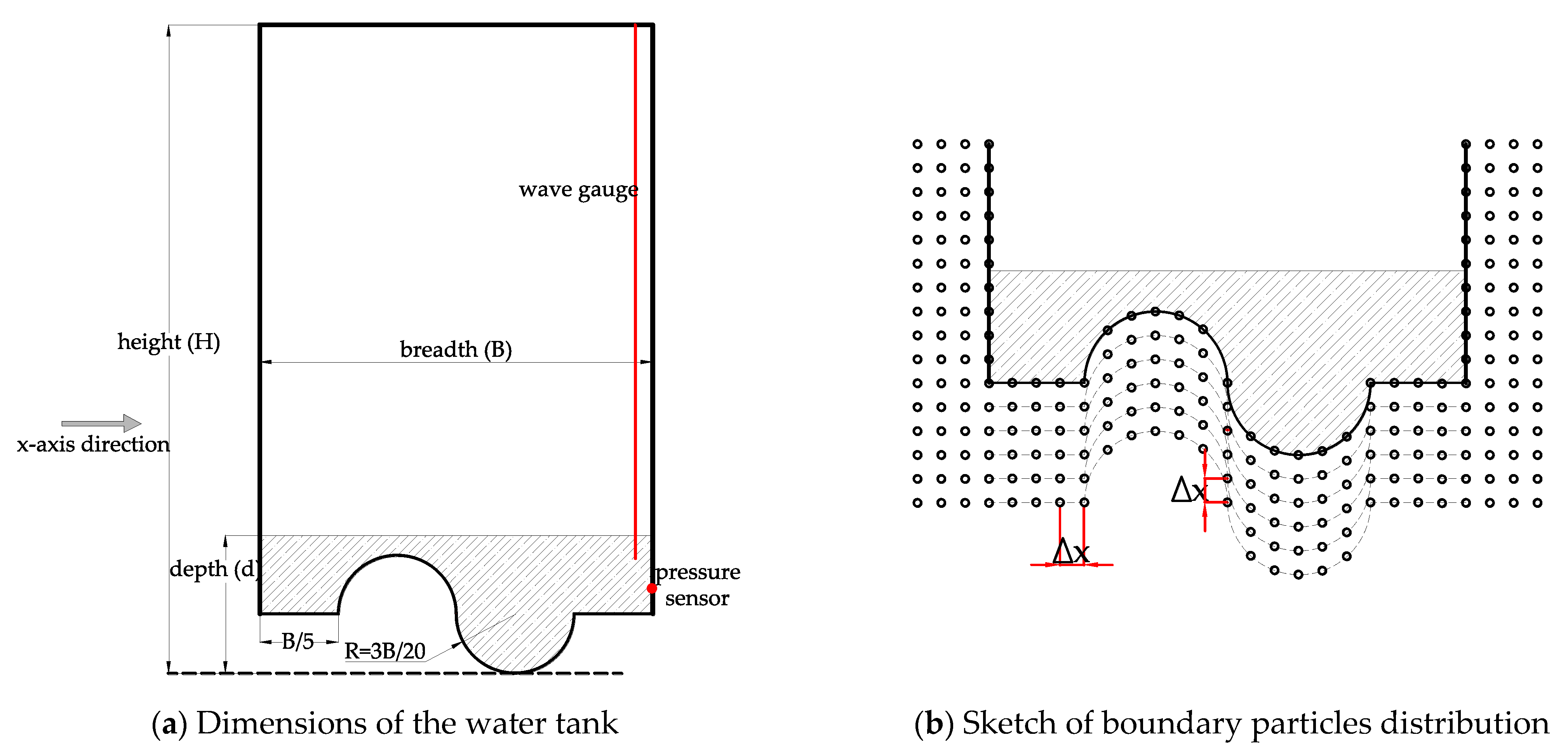
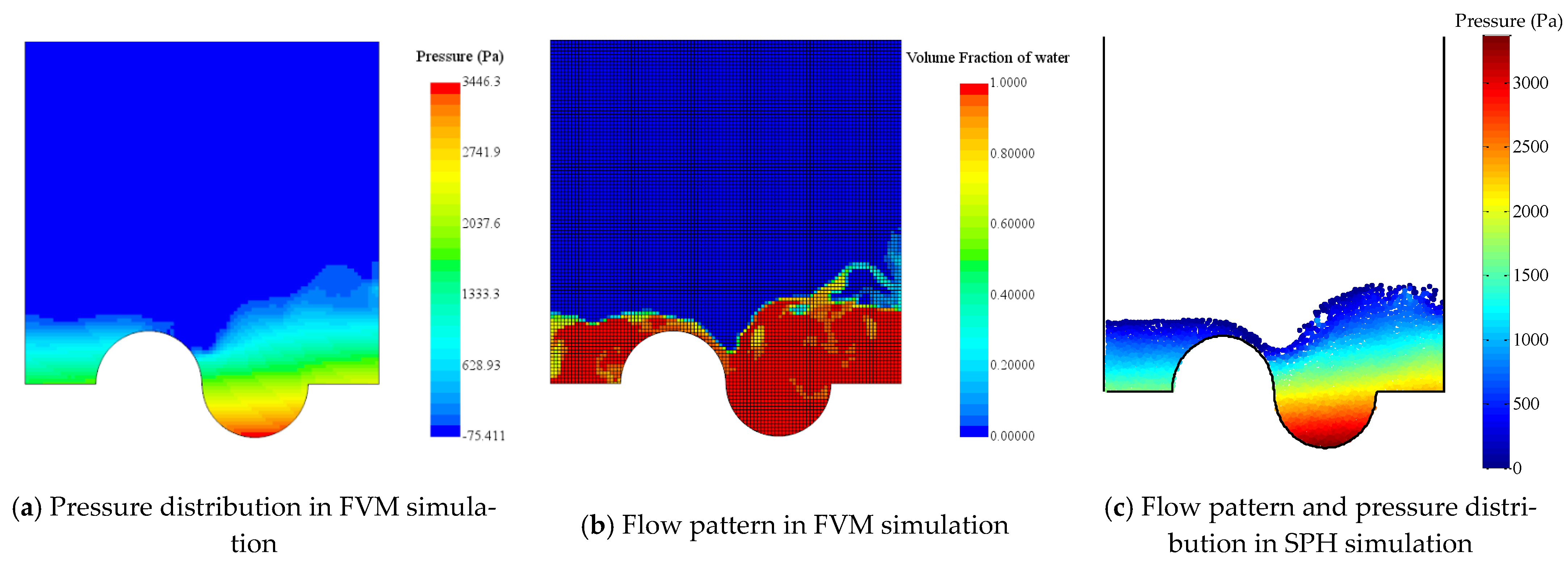
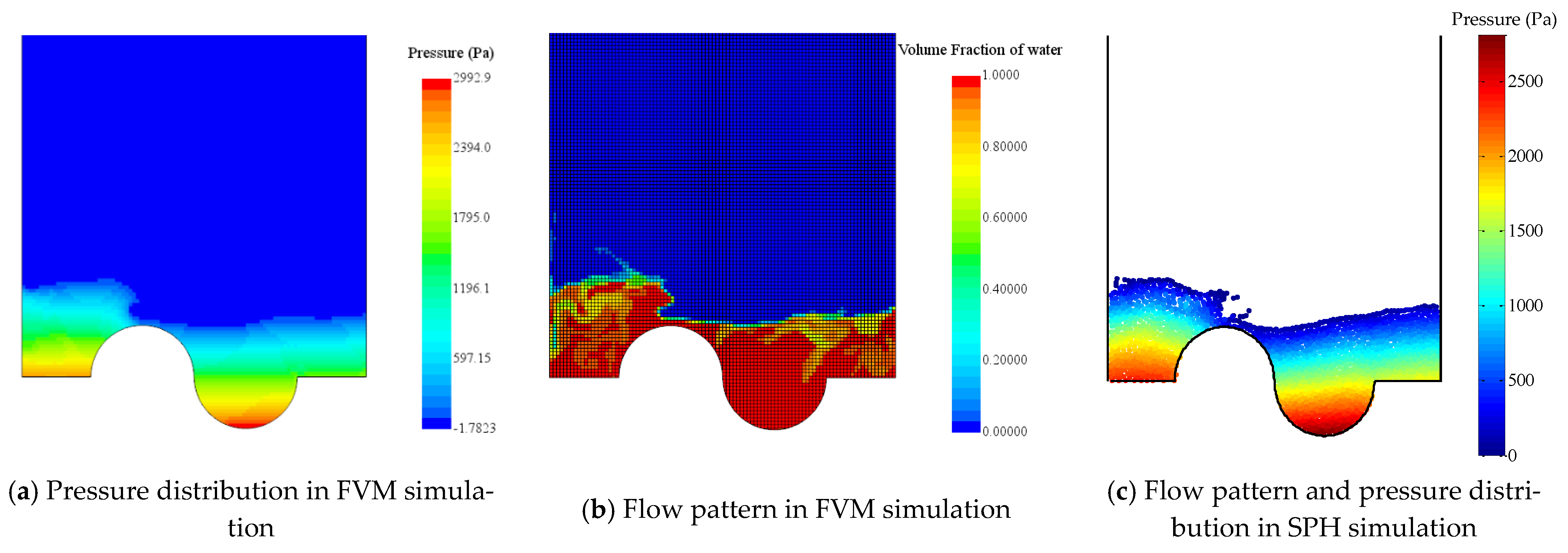
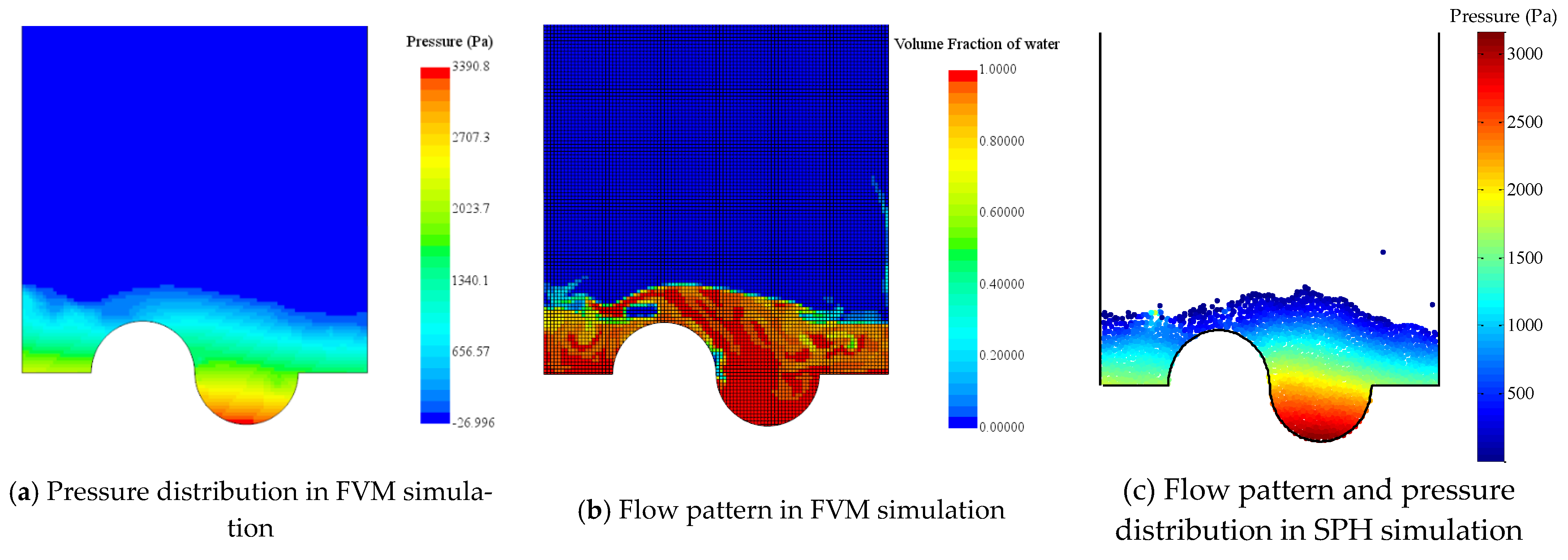
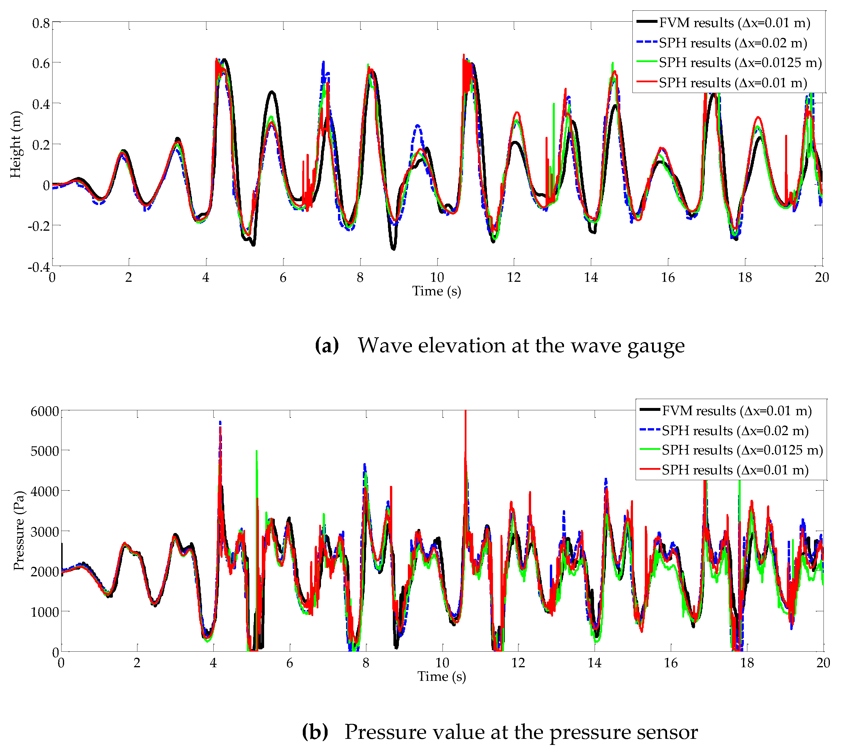
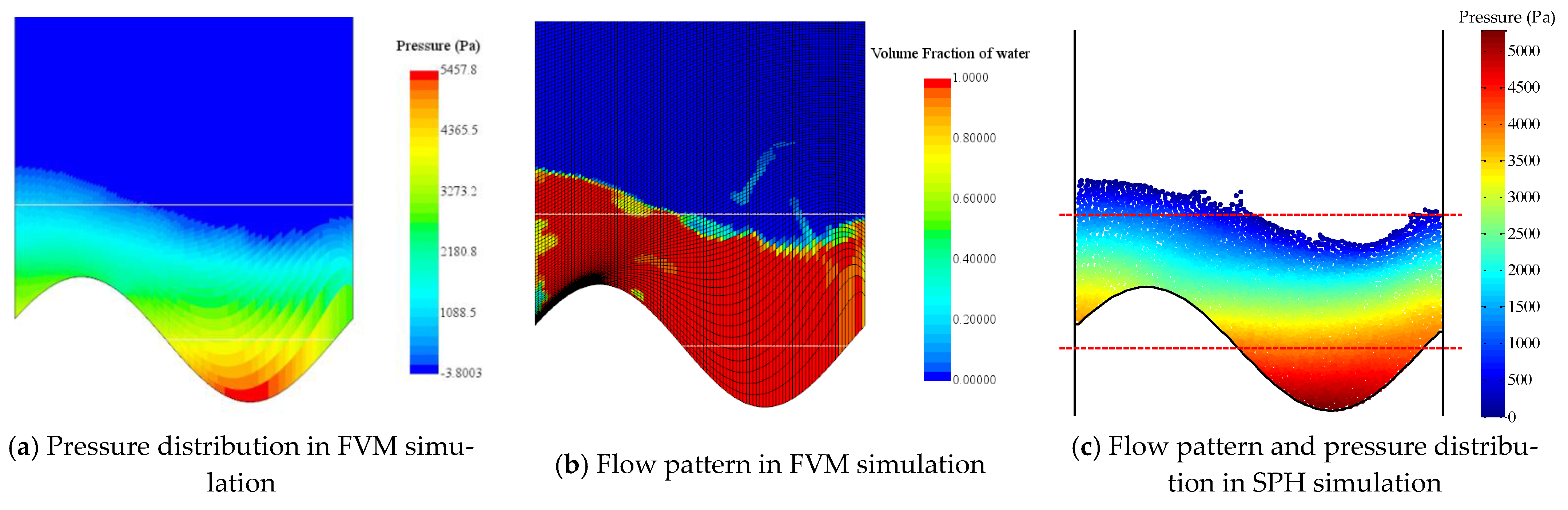
4.3. Sloshing in Tanks with Complex Geometry

Violent sloshing simulations in tank with complex geometry are conducted with FVM and SPH with different boundary methods. The geometry of the sloshing tank is shown in Figure 9a. The tank breadth, height and initial water depth are 1.0 m, 1.65 m and 0.45 m, respectively. The radius of the semicircles is 0.15 m. A pressure sensor is placed 0.1 m below the initial free surface on the right wall, and a wave gauge is placed 0.01 m from the right wall, as shown in Figure 9a. For the lateral acceleration $a\left(t\right)=\lambda A{\omega }^2\sin \left(\omega t\right)$, the amplitude of displacement is 0.01 m and the excitation frequency is 4.0 rad/s. In the SPH simulations, the numerical sound speed is $c_s=17\mathrm{m}/\mathrm{s}$, and the other SPH parameters are as the same with those in previous sloshing cases in Section 4.2. The particle spacing is set to $\Delta x=0.01\mathrm{m}$, resulting in about 2009 fluid particles generated in the computation domain. In the FVM simulation, the grid spacing is set the same as the particle spacing used in SPH simulation, and other parameters are the same as these in the FVM simulation of Section 4.2. It should be noted that although FVM is well validated in Section 4.2, FVM still has some problems for violent sloshing simulations with dynamically evolving free surface, and the free surface is difficult to be accurately captured.

The sketch of boundary particles distribution around the tank’s bottom is shown in Figure 9b. It is obvious that the boundary particles distribution is a little coarse due to the restrictions of the tank’s geometry. If the boundary methods used do not have a strong ability of preventing fluid particles penetration, fluid particles can easily cross the solid wall under violent sloshing excitation.

In the SPH simulations with the previous SBT algorithms used by Shao et al. and Chen et al., at least more than 450 (22%) fluid particles penetrate the solid wall from the gap between boundary particles during the 60 s simulation. As shown in Figure 10, the SPH results of the simulation with the previous SBT algorithms are less accurate and reliable. However, in the SPH simulation with the new SBT algorithm, no fluid particle penetration occurs throughout the entire simulation, and the SPH results obtained with the new boundary method agree well with the FVM results. The reason is that the magnitude of the repulsive forces in the previous SBT algorithm only depends on the distance between the fluid particle and the repulsive particle. In the new SBT algorithm, the magnitude of the repulsive forces, produced by the repulsive particle, not only depends on the distance between the fluid particle and the repulsive particle, but also the distance between the fluid particle and the plane to which the repulsive particle belongs. Obviously, the repulsive force in the new SBT algorithm, partially based on the plane, has better ability of preventing particle penetration than that in the previous SBT algorithm.

Besides, it should be noted here that, the criterion for determining fluid particle penetration in the SPH simulation with the new SBT algorithm is different from that in the SPH simulations with the previous SBT algorithms. For the new SPH scheme in this study, fluid particles that completely leave the outermost layer of the computation domain will be marked as penetration particles and removed from the computation domain. In the simulations with the previous SBT algorithms, fluid particles that penetrate the inner layer of boundary particles at the solid wall will be removed from the computation domain. If the same criterion as used in the new SPH scheme, the SPH simulations with the previous SBT algorithms will break, and the 60 s simulation cannot be accomplished because of too many fluid particles penetration occurrences.

Figure 11, Figure 12 and Figure 13 show the comparisons of the flow pattern and pressure distribution from the FVM simulation and SPH simulations at some typical instants. The flow field in SPH simulations is in general consistent with that in FVM simulation. As shown in Figure 11b, Figure 12b and Figure 13b of the FVM simulation, the interface between water and air is not clear under so violent sloshing excitation. But the flow fields in SPH simulations are still stable and smooth, and the SPH results obtained using the new SBT algorithm are close to the FVM results for the pressure histories and wave elevation at the probes, as shown in Figure 10. The advantage and robustness of the new SBT algorithm can be validated by the violent sloshing simulation with coarse boundary particles distribution.

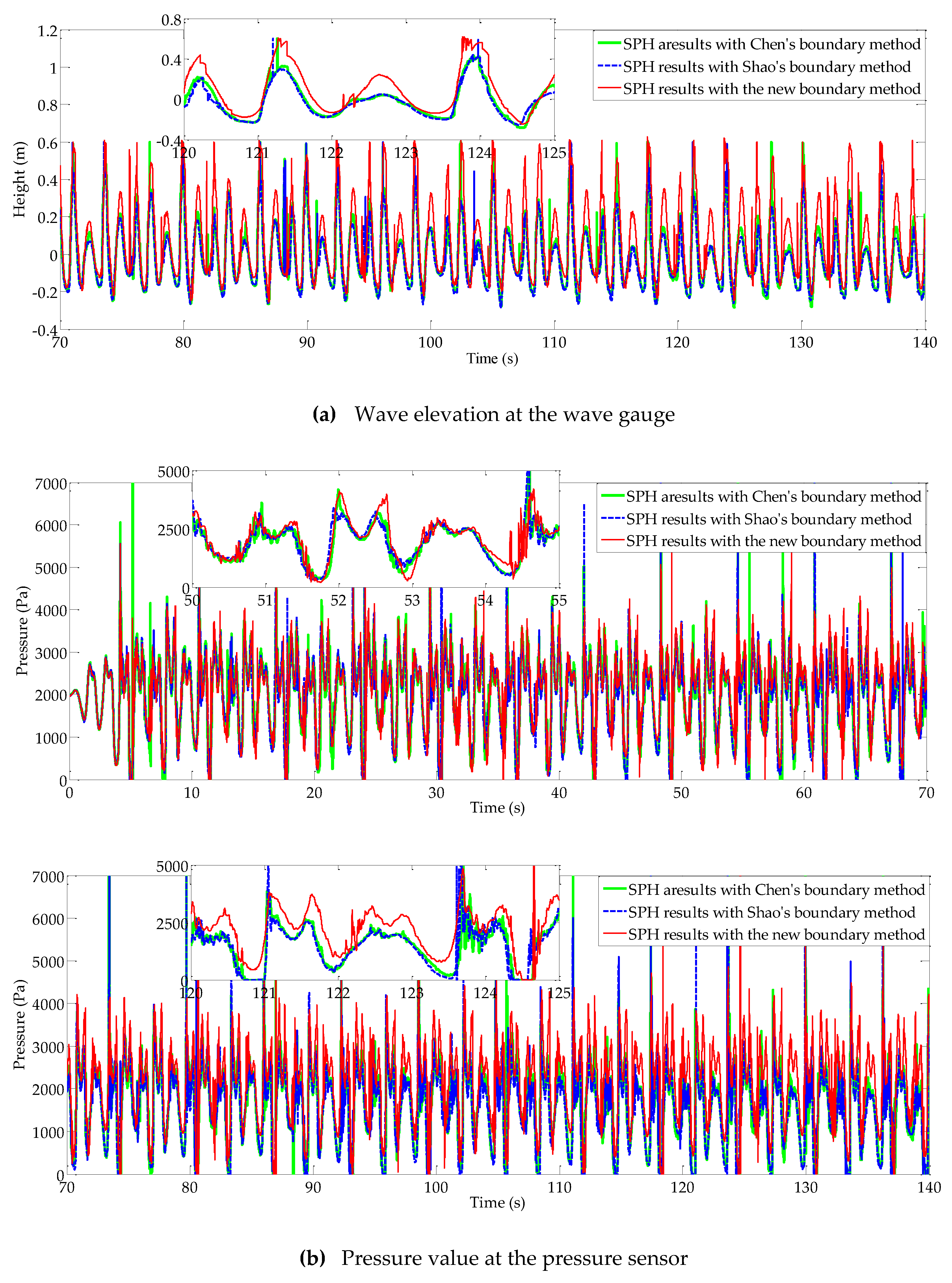
4.4. Sloshing in Tank with Unidirectional Deformable Boundaries

Modelling deformable boundaries is quite a problem for these fixed ghost particle boundary methods. To investigate the performance of the new SBT algorithm in simulating deformable boundaries, a case of sloshing in water tank with unidirectional deformable bottom is simulated by both SPH and FVM. The dimensions of the tank are shown in Figure 14a. The tank is 1.0 m wide and 2.0 m high, which is large enough to make sure that no water particle can reach the ends. The initial water depth is 0.4 m, and the initial position of the deformable bottom is 0.5 m above the ground. A pressure probe point is placed 0.2 m below the initial free surface on the right wall, and a wave probe is placed 0.01 m from the right wall, as shown in Figure 14a. The tank’s motion is driven by a horizontal excitation and a vertical excitation of the deformable bottom. In the horizontal direction, the excitation pattern of the tank is as the same as the tank’s motion of the sloshing case in Section 4.2. The amplitude of displacement $A$ is set to 0.03 m and the excitation frequency $\omega$ is 5.0 rad/s. In the vertical direction, the deformation of the tank’s bottom is controlled by the deformation velocity:

$$v\left(x,t_v\right)=\lambda A_v\cos \left(k_{v}x-{\omega }_v{t}_v\right)$$

(12)

where ${\omega }_v$ is the frequency, $A_v$ the amplitude and $k_v$ the wave number. In this study, the deformable motion parameters of the tank’s bottom are ${\omega }_v=2.0\mathrm{rad}/\mathrm{s}$, $A_v=0.2\mathrm{m}$ and $k_v=2\pi$. It should be noted that the time step of boundary deformation $d{t}_v$ in SPH simulation is set 100 times of the time step $dt$ of the Predictor-Corrector scheme. During the time step $d{t}_v$, the deformation velocity of the bottom is approximately regarded as constant for the calculation of the physical quantities of fluid particles, as which can greatly improve the numerical stability of the SPH simulation. Figure 14b shows the initial distribution of particles in the tank. The bottom boundary particles move with the deformable bottom, as shown in Figure 14c.

In the SPH simulations, to examine the convergence of the SPH scheme, three different particle spacings are explored in these SPH simulations, $\Delta x=0.02\mathrm{m}$, $\Delta x=0.0125\mathrm{m}$ and $\Delta x=0.01\mathrm{m}$, resulting in about 980, 2528 and 3960 fluid particles in the computation domain. The time step $dt$ is set to $5\times {10}^{-5}\mathrm{s}$ for all SPH simulations. The deformation time step $d{t}_v$ is set to 0.005 s, which is an acceptable approximation of deformation velocity. The density of water is $\rho =1000{\mathrm{kg}/\mathrm{m}}^3$, the numerical sound speed is $c_s=12\sqrt{gd}$, the artificial viscosity coefficient is $\alpha =0.02$. The MLS correction of density field is applied at every time step for both fluid particles and boundary particles, which is more frequent than these sloshing simulations in Section 4.2 and Section 4.3. Since the deformable boundary can intensify particles clumping and numerical dissipation, the particle shifting correction is applied to improve the fluid particles distribution. The particle shifting coefficient $A_s$ is a little different for different particle spacings. In the SPH simulation with $\Delta x=0.02\mathrm{m}$, the particle shifting coefficient $A_s$ is set to 0.8. While in the other SPH simulations, the particle shifting coefficient $A_s$ is 0.3.

As for the FVM simulations, the sloshing simulations are conducted with the commercial code STAR-CCM+ using the Euler two-phase separated flow model. The STAR-CCM+ contains a morphing motion model that can be used to define the deformable motion of the tank’s bottom [37]. Three different grid spacings are explored, which are the same as the particle spacings used in the SPH simulation. For the purpose of convenience, the time step of all the three FVM simulations is set to 0.001 s, which satisfies the Courant condition. As shown in Figure 15, the results of the three FVM simulations in 20 s converge reasonably well, although some discrepancies which are caused by jet flow near the wall boundary appear in Figure 15a. Thus, the results of the FVM simulation with grid spacing $\Delta x=0.01\mathrm{m}$ are chosen as the benchmark value.

In order to examine the convergence of the new SPH scheme in this study, three SPH simulations with different particle spacings are conducted. Figure 16 shows the comparisons of SPH results and the FVM results for the wave elevation and pressure on the measuring probes in 20 s. The SPH results obtained with $\Delta x=0.01\mathrm{m}$ agree most with the FVM results, as shown in Figure 16. Figure 17 and Figure 18 show the comparisons of the typical flow pattern and pressure distribution for the FVM simulation and SPH simulation at two typical instants. The SPH results are highly consistent with the results of FVM. Some slight discrepancies are present in Figure 17, because the air cavity only can be captured in the FVM simulation based on the Euler two-phase flow model. The pressure fields of the SPH simulation with the new SBT algorithm are smooth, and almost no particle penetration occurs. It can be concluded that, with the new SBT algorithm, the SPH scheme in this study has the ability of simulating sloshing cases with unidirectional deformable boundary.

To compare the new SBT algorithm with previous ones, the SPH simulations with different coupled dynamic SBT algorithms are conducted for 140 s. Although fluid particles penetration also appears in the SPH simulation using the new SBT algorithm, the number of fluid particles penetrating the wall boundary is much smaller than those using the previous SBT algorithms, as shown in

Table 3. Numbers of penetration particles in the SPH simulations.

	Time	20 s	60 s	100 s	140 s
Cases
New boundary method		2	3	5	5
Boundary method by Chen		122	352	641	863
Boundary method by Shao		155	469	744	953

. A great improvement in the ability of preventing fluid particles penetration is observed. It should be noted that, at the initial state of the SPH simulation with $\Delta x=0.01\mathrm{m}$, there are 3960 fluid particles in the fluid domain. Figure 19 shows the results of the liquid sloshing SPH simulations. Since the grid distortion in FVM simulation after 20 s is gradually becoming severe as the simulation goes, the FVM results are less accurate and not present in Figure 19. As the SPH simulation goes, more and more fluid particles penetrate the wall boundary and are removed from the computation domain in the SPH simulation using the previous SBT algorithms. The discrepancy between the SPH results with the new SBT algorithm and the previous SBT algorithms is becoming more and more obvious along with the increase of the number of penetration fluid particles, as shown in Figure 19.

In this section, the sloshing simulations in the tank with both horizontal translational excitation and deforming bottom excitation are conducted using the new SPH scheme. The numerical stability and accuracy of the new SBT algorithm are demonstrated, even for complicated and violent sloshing cases. Success in obtaining stable and accurate numerical results is attributed to the repulsive force of repulsive particles and the relatively uniform fluid particle distribution near the boundaries.

5. Conclusions

In the present study, a novel improved coupled dynamic SBT is proposed to model the boundaries for 2D SPH sloshing simulation. Several sloshing simulations are conducted for investigating the numerical stability and accuracy of the new SBT algorithm, including sloshing in tank with unidirectional deformable boundaries. Based on the simulations and analysis, the following conclusions can be drawn.

(1)

The improvement in the ability to prevent fluid particles penetration is achieved in the new SBT algorithm by improving the formulation of the repulsive forces, which enables the boundary method to simulate violent sloshing cases with complex geometries. Besides, comparing with the previous SBT algorithm, the numerical dissipation in these simulations with the new SBT algorithm is obviously reduced.

(2)

With the new SBT algorithm, the SPH scheme in this study can be used to simulate sloshing cases with unidirectional deformable boundary. The new SBT algorithm produces results with better numerical stability than the previous SBT algorithms.

(3)

The numerical stability and accuracy of the new SBT algorithm is validated for liquid sloshing cases. The numerical results obtained by the SPH scheme are in satisfactory agreement with the experimental results or FVM results calculated by STAR-CCM+. Besides, the new SBT algorithm shows great potential in the application of fluid-structure interaction problems.

References

1. Nasar, A.M. Eulerian and Lagrangian Smoothed Particle Hydrodynamics as Models for the Interaction of Fluids and Flexible Structures in Biomedical Flows; The University of Manchester: Manchester, UK, 2016. [Google Scholar]
2. Gingold, R.A.; Monaghan, J.J. Smoothed particle hydrodynamics: Theory and application to non-spherical stars. Mon. Not. R. Astron. Soc. 1977, 181, 375–389. [Google Scholar] [CrossRef]
3. Lin, J.; Naceur, H.; Coutellier, D.; Laksimi, A. Efficient meshless SPH method for the numerical modeling of thick shell structures undergoing large deformations. Int. J. Non-Linear Mech. 2014, 65, 1–13. [Google Scholar] [CrossRef]
4. Liu, M.; Liu, G. Smoothed particle hydrodynamics (SPH): An overview and recent developments. Arch. Comput. Methods Eng. 2010, 17, 25–76. [Google Scholar] [CrossRef] [Green Version]
5. Iglesias, A.S.; Rojas, L.P.; Rodríguez, R.Z. Simulation of anti-roll tanks and sloshing type problems with smoothed particle hydrodynamics. Ocean Eng. 2004, 31, 1169–1192. [Google Scholar] [CrossRef]
6. Souto-Iglesias, A.; Delorme, L.; Pérez-Rojas, L.; Abril-Pérez, S. Liquid moment amplitude assessment in sloshing type problems with smooth particle hydrodynamics. Ocean Eng. 2006, 33, 1462–1484. [Google Scholar] [CrossRef]
7. Chen, Z.; Zong, Z.; Liu, M.; Li, H. A comparative study of truly incompressible and weakly compressible SPH methods for free surface incompressible flows. Int. J. Numer. Methods Fluids 2013, 73, 813–829. [Google Scholar] [CrossRef] [Green Version]
8. Monaghan, J.J.; Rafiee, A. A simple SPH algorithm for multi-fluid flow with high density ratios. Int. J. Numer. Methods Fluids 2013, 71, 537–561. [Google Scholar] [CrossRef]
9. Dincer, A.E. Investigation of the sloshing behavior due to seismic excitations considering two-way coupling of the fluid and the structure. Water 2019, 11, 2664. [Google Scholar] [CrossRef] [Green Version]
10. Trimulyono, A.; Hashimoto, H.; Matsuda, A. Experimental validation of single-and two-phase smoothed particle hydrodynamics on sloshing in a prismatic tank. J. Mar. Sci. Eng. 2019, 7, 247. [Google Scholar] [CrossRef] [Green Version]
11. Gabl, R.; Davey, T.; Ingram, D.M. Roll Motion of a Water Filled Floating Cylinder—Additional Experimental Verification. Water 2020, 12, 2219. [Google Scholar] [CrossRef]
12. Kocaman, S.; Dal, K. A New Experimental Study and SPH Comparison for the Sequential Dam-Break Problem. J. Mar. Sci. Eng. 2020, 8, 905. [Google Scholar] [CrossRef]
13. Tran-Duc, T.; Meylan, M.H.; Thamwattana, N.; Lamichhane, B.P. Wave Interaction and Overwash with a Flexible Plate by Smoothed Particle Hydrodynamics. Water 2020, 12, 3354. [Google Scholar] [CrossRef]
14. Qian, L.; Causon, D.M.; Mingham, C.G.; Ingram, D.M. A free-surface capturing method for two fluid flows with moving bodies. Proc. R. Soc. A Math. Phys. Eng. Sci. 2006, 462, 21–42. [Google Scholar] [CrossRef]
15. Lee, D.; Kim, M.; Kwon, S.; Kim, J.; Lee, Y. A parametric sensitivity study on LNG tank sloshing loads by numerical simulations. Ocean Eng. 2007, 34, 3–9. [Google Scholar] [CrossRef]
16. Chen, Z.; Zong, Z.; Li, H.; Li, J. An investigation into the pressure on solid walls in 2D sloshing using SPH method. Ocean Eng. 2013, 59, 129–141. [Google Scholar] [CrossRef]
17. Fourtakas, G.; Dominguez, J.M.; Vacondio, R.; Rogers, B.D. Local uniform stencil (LUST) boundary condition for arbitrary 3-D boundaries in parallel smoothed particle hydrodynamics (SPH) models. Comput. Fluids 2019, 190, 346–361. [Google Scholar] [CrossRef]
18. Monaghan, J.J. Simulating free surface flows with SPH. J. Comput. Phys. 1994, 110, 399–406. [Google Scholar] [CrossRef]
19. Kulasegaram, S.; Bonet, J.; Lewis, R.; Profit, M. A variational formulation based contact algorithm for rigid boundaries in two-dimensional SPH applications. Comput. Mech. 2004, 33, 316–325. [Google Scholar] [CrossRef]
20. Randles, P.; Libersky, L.D. Smoothed particle hydrodynamics: Some recent improvements and applications. Comput. Methods Appl. Mech. Eng. 1996, 139, 375–408. [Google Scholar] [CrossRef]
21. Crespo, A.J.; Gómez-Gesteira, M.; Dalrymple, R.A. Boundary conditions generated by dynamic particles in SPH methods. Comput. Mater. Contin. 2007, 5, 173–184. [Google Scholar]
22. Adami, S.; Hu, X.Y.; Adams, N.A. A generalized wall boundary condition for smoothed particle hydrodynamics. J. Comput. Phys. 2012, 231, 7057–7075. [Google Scholar] [CrossRef]
23. Shao, J.; Li, H.; Liu, G.; Liu, M. An improved SPH method for modeling liquid sloshing dynamics. Comput. Struct. 2012, 100, 18–26. [Google Scholar] [CrossRef] [Green Version]
24. Liu, M.; Shao, J.; Chang, J. On the treatment of solid boundary in smoothed particle hydrodynamics. Sci. China Technol. Sci. 2012, 55, 244–254. [Google Scholar] [CrossRef]
25. Cao, X.; Ming, F.; Zhang, A. Sloshing in a rectangular tank based on SPH simulation. Appl. Ocean Res. 2014, 47, 241–254. [Google Scholar] [CrossRef]
26. Green, M.D.; Peiró, J. Long duration SPH simulations of sloshing in tanks with a low fill ratio and high stretching. Comput. Fluids 2018, 174, 179–199. [Google Scholar] [CrossRef]
27. Crespo, A.; Dominguez, J.; Gómez-Gesteira, M.; Barreiro, A.; Rogers, B. User Guide for DualSPHysics Code; University of Vigo: Vigo, Spain; The University of Manchester: Manchester, UK; Johns Hopkins University: Baltimore, MD, USA, 2011. [Google Scholar]
28. Monaghan, J.J. Smoothed particle hydrodynamics. Annu. Rev. Astron. Astrophys. 1992, 30, 543–574. [Google Scholar] [CrossRef]
29. Colagrossi, A.; Landrini, M. Numerical simulation of interfacial flows by smoothed particle hydrodynamics. J. Comput. Phys. 2003, 191, 448–475. [Google Scholar] [CrossRef]
30. Lind, S.J.; Xu, R.; Stansby, P.K.; Rogers, B.D. Incompressible smoothed particle hydrodynamics for free-surface flows: A generalised diffusion-based algorithm for stability and validations for impulsive flows and propagating waves. J. Comput. Phys. 2012, 231, 1499–1523. [Google Scholar] [CrossRef]
31. Skillen, A.; Lind, S.; Stansby, P.K.; Rogers, B.D. Incompressible smoothed particle hydrodynamics (SPH) with reduced temporal noise and generalised Fickian smoothing applied to body–water slam and efficient wave–body interaction. Comput. Methods Appl. Mech. Eng. 2013, 265, 163–173. [Google Scholar] [CrossRef]
32. Gomez-Gesteira, M.; Rogers, B.D.; Dalrymple, R.A.; Crespo, A.J. State-of-the-art of classical SPH for free-surface flows. J. Hydraul. Res. 2010, 48, 6–27. [Google Scholar] [CrossRef]
33. Pa’ kozdi, C.; Graczyk, M. Validation of an SPH sloshing simulation by experiments. In Proceedings of the 28th International Conference on Ocean, Offshore and Arctic Engineering, Honolulu, HI, USA, 31 May–5 June 2009; pp. 729–739. [Google Scholar]
34. Cao, Y.; Graczyk, M.; Pakozdi, C.; Lu, H.; Huang, F.; Yang, C. Sloshing Load Due to Liquid Motion in a Tank Comparison of Potential Flow, CFD, and Experiment Solutions. In Proceedings of the Twentieth International Offshore and Polar Engineering Conference, Beijing, China, 20–25 June 2010. [Google Scholar]
35. Benson, D.J.; Ng, W. Validation of Slosh Modeling Approach Using STAR-CCM+. 2018. Available online: https://ntrs.nasa.gov/citations/20180003007 (accessed on 17 November 2021).
36. Li, C.B.; Choung, J. Numerical and Experimental Study on Sloshing Impact Loads in IMO Type-C LNG Tanks with Different Swash Bulkheads. In Practical Design of Ships and Other Floating Structures; Springer: Singapore, 2019; pp. 1046–1055. [Google Scholar]
37. User Guide. STAR-CCM+ Version (10.02); CD-Adapco: New York, NY, USA, 2015. [Google Scholar]
Figure 1. Illustration of (a) the previous coupled dynamic SBT algorithm and (b) the new coupled dynamic SBT algorithm (the black solid line denote the wall boundary; the red node is the fluid particle; the green square represent the boundary particle of concern; the split red circle represent the support domain of the boundary particle, and the physical quantities of particles in the solid part are used to calculate the boundary particle’s physical quantities, details shown in references [16,23,24]. Figure 1a is from references [16,23,24]).
Jmse 09 01395 g001aJmse 09 01395 g001b
Figure 2. Pressure field and particle distribution at 15.0 s: (a) SPH results with Chen’s boundary method; (b) SPH results with Shao’s boundary method; (c). SPH results with the new boundary method.
Jmse 09 01395 g002
Figure 3. Pressure histories at the pressure sensor.
Jmse 09 01395 g003
Figure 4. Comparisons of particle pressure values versus depth obtained by SPH simulations with different boundary methods at 15.0: (a) SPH results with Chen’s boundary method; (b) SPH results with Shao’s boundary method; (c) SPH results with the new boundary method.
Jmse 09 01395 g004
Figure 5. Dimensions of the water tank.
Jmse 09 01395 g005
Figure 6. Wave elevation at the wave gauge obtained by the numerical simulations and experiment of (a) Case 1 and (b) Case 2.
Jmse 09 01395 g006aJmse 09 01395 g006b
Figure 7. Pressure values at the pressure sensor obtained by the numerical simulations and experiment of (a) Case 1 and (b) Case 2.
Jmse 09 01395 g007
Figure 8. Pressure values at the pressure sensor obtained by the numerical simulations for Case 1: (a) SPH results with Chen’s boundary method; (b) SPH results with Shao’s boundary method; (c) SPH results with the new boundary method.
Jmse 09 01395 g008aJmse 09 01395 g008b
Figure 9. Configuration of the water tank: (a) Dimensions of the water tank; (b) Sketch of boundary particles distribution.
Jmse 09 01395 g009
Figure 10. Numerical results obtained by FVM simulation and SPH simulations: (a) Wave elevation at the wave gauge; (b) Pressure value at the pressure sensor.
Jmse 09 01395 g010
Figure 11. Comparisons of the flow pattern and pressure distribution at 10.0 s: (a) Pressure distribution in FVM simulation; (b) Flow pattern in FVM simulation; (c) Flow pattern and pressure distribution in SPH simulation.
Jmse 09 01395 g011
Figure 12. Comparisons of the flow pattern and pressure distribution at 19.0 s: (a) Pressure distribution in FVM simulation; (b) Flow pattern in FVM simulation; (c) Flow pattern and pressure distribution in SPH simulation.
Jmse 09 01395 g012
Figure 13. Comparisons of the flow pattern and pressure distribution at 29.4 s: (a) Pressure distribution in FVM simulation; (b) Flow pattern in FVM simulation; (c) Flow pattern and pressure distribution in SPH simulation.
Jmse 09 01395 g013
Figure 14. Configuration of the water tank: (a) Dimensions of the water tank; (b) Initial particles distribution in the tank; (c) Sketch of boundary particles distribution.
Jmse 09 01395 g014
Figure 15. Numerical results obtained by FVM simulations: (a) Wave elevation at the wave gauge; (b) Pressure value at the pressure sensor.
Jmse 09 01395 g015
Figure 16. Numerical results obtained by FVM simulation and SPH simulations: (a) Wave elevation at the wave gauge; (b) Pressure value at the pressure sensor.
Jmse 09 01395 g016
Figure 17. Comparisons of the flow pattern and pressure distribution at 7.8 s: (a) Pressure distribution in FVM simulation; (b) Flow pattern in FVM simulation; (c) Flow pattern and pressure distribution in SPH simulation.
Jmse 09 01395 g017
Figure 18. Comparisons of the flow pattern and pressure distribution at 18.0 s: (a) Pressure distribution in FVM simulation; (b) Flow pattern in FVM simulation; (c) Flow pattern and pressure distribution in SPH simulation.
Jmse 09 01395 g018
Figure 19. Numerical results obtained by SPH simulations: (a) Wave elevation at the wave gauge; (b) Pressure value at the pressure sensor.
Jmse 09 01395 g019aJmse 09 01395 g019b