Satellite Observation of the Marine Light-Fishing and Its Dynamics in the South China Sea

Abstract

The South China Sea (SCS) is one of the most important fishery resource bases in the world. Marine fisheries, as a crucial component of regional food security and national revenue, raise wide concern about marine ecology, social-economic and political consequences at regional, national and local scales. The large-scale dynamic detection and analysis of fishing activity in the SCS is still unclear because of the accessibility of in-site data, finite automatic identification system (AIS) usage, complex geopolitics and poor additional data coverage. Nighttime light imagery (NTL) derived from low light imaging sensors and the popularity of light fishing in the SCS offers a unique way to unveil fishing activities and its dynamics. In this study, we proposed a set of algorithms for automatic detection of nighttime fishing activity and provided the first large-scale dynamic analysis of nighttime fishing activity in the SCS using monthly Visible Infrared Imaging Radiometer Suite (VIIRS) images between 2012 and 2019. The proposed method effectively minimized the spatio-temporal fluctuations in radiance values of background and their implications to ship detection by integrating high radiance gradient detection and local adaptive thresholding. Further, nighttime fishing activity trajectories were decomposed into trend and seasonal components by using Hilbert-Huang transformation (HHT) to accurately access general trends and the seasonality of nighttime fishing activity in the SCS. The typical subregions analysis, environmental driver analysis, correlation coefficient analysis and hot spot analysis were integrated to characterize the nighttime fishing activity. It appears that the nighttime fishing activity in the SCS exhibited spatio-temporal variability and heterogeneity and was shaped by policy and natural factors such as holidays, annual Chinese fishery moratoria in the Chinese Exclusive Economic Zone (EEZ) and seasonal tropical storm activity.

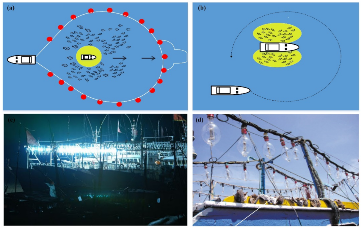
1. Introduction

The South China Sea (SCS) is one of the most important fishery resource bases in the world. It remains one of the top five most productive fishing areas in the world in terms of fisheries catch and simultaneously possesses immense marine aquaculture production quantity [1]. From the late 1980s to the early 1990s, fishery product exports from the SCS comprised an average of 11% of annual world exports, increasing to 27% by 2011. Fisheries resources in the SCS play a crucial role in marine ecology, coastal livelihoods, food security, and export trade to surrounding countries [2,3].

Over the past few decades, SCS fisheries have faced substantial challenges such as growing fishing pressures, excessive fishing capacity, and widespread overexploitation following rapid expansion of industrial fishing [4]. The unsustainable status spurred a series of socio-economic, political and ecological problems such as declining fish catches [4], the growing proportion of overfished or fully fished species [4,5], escalation in fisheries and territorial dispute [4], marine habitat and biodiversity loss [6,7], alteration of ecosystem trophic structures [7] and potential food security/livelihood issues [1,8]. Hence, the present situation reiterates the urgency for understanding and monitoring of fishing activity in the SCS.

Against this backdrop, a series of fishery studies has been made using various analysis such as fishing stock assessments, fishing-related habitat analysis and spatio-temporal analysis of fishing resources [9,10,11,12,13,14,15,16,17,18,19,20]. However, most studies in the SCS preferred an analysis of the small-scale fisheries at a single or inconsistent time [4,6,21,22,23,24,25,26,27,28,29,30,31,32,33,34,35,36,37,38,39] and few attempts have been made to investigate large-scale fishery dynamics and access their regularity. Lacking large-scale consistent time-series fishery data is a main reason for this scarcity. In the SCS, fishery statistical data are neither publicly available nor global in scope because of the complex geopolitics and accessibility of in situ data. The widely used automatic identification system (AIS) dataset suffers from several limitations that impact its effectiveness in investigating fishing dynamics. The key limitation includes limited AIS usage in the SCS and a potential misreporting issue of AIS data [40,41]. Despite its high spatial and temporal resolution, AIS coverage is biased toward industrial fisheries and wealthier countries and AIS data lacks records of small-scale fisheries [40]. In addition, radio interference in the case of a dense vessel population and closure of AIS device for security or manual operations impaired the estimation of fishing activity. Normal spectral bands are not appropriate for fishing vessel recognition because of fuzzy features or blurry detections in optical images.

Artificial nighttime lights (NTL) offer a new way to unveil human activities and dynamics [42,43,44,45,46,47,48,49,50,51,52,53,54,55,56,57,58,59,60]. It has been known since the 1970s that anthropogenic lighting present at the earth’s surface at night can be detected by low light imaging sensors onboard environmental satellites [44]. NTL images derived from low light imaging sensors, particularly the Defense Meteorological Satellite Program/Operational Linescan (DMSP/OLS) have been widely used to characterize socio-economic activity due to data availability and the superiority of wide spatial coverage, relatively long temporal span and little interference by shadows. Light fishing, placing rows (lines) of high-power lights on the surface or underwater to attract fish based on their phototaxis (Figure 1), has been one of the most widespread modern fishing methods. Light emissions generated by nighttime fishing activity, reaching up to hundreds of kilowatts, can be easily detected by low light imagers. In the SCS, light fishing can be categorized into four groups: falling-net, trawling, longline and purse seining. Light falling-net fishing has been widely used by many countries since the 1990s (in the northern SCS). Light purse seining fishing was the most widespread activity in the SCS [41] and had much more abundant catch than other fishing types. To increase the efficiency of purse seining fishing, several auxiliary vessels undertake the mission of attracting and guiding fish to the fishing net in close conjunction with the main fishing vessel (Figure 1). These provide the feasibility of monitoring and investigating large-scale fishing activity in the SCS.

Previous studies have demonstrated the feasibility and capability of DMSP/OLS imagery for fishery studies [61,62,63]. However, DMSP imagery has a set of shortcomings: a coarse spatial resolution (2.7 km), non-radiometric calibration with low radiometric resolution (6 bit), saturation and blooming effects, and lacking spectral channels suitable for discrimination of thermal sources of lighting [64]. These shortcomings impact its effectiveness and accuracy in fishery simulation and analysis. Such limitations have been alleviated with the successful launch of the Suomi National Polar-orbiting Partnership (Suomi NPP, launched on October 28, 2011) due to the superiority of a higher spatial (742 m) and radiometric resolution (14 bit), rigorous calibration system and reduced spatial blurring and pixel saturation for the new NTL data [64,65,66,67]. Visible Infrared Imaging Radiometer Suite (VIIRS), one of five sensors onboard the Suomi NPP satellite, carried a unique Day/Night Band (DNB) radiometer, collecting both visible and near-infrared light (500–900 nm) during both day and night. It is highly sensitive to faint light in its band pass, even the light emitted from an isolated street lamp on its orbital altitude [68,69]. Additionally, DNB imagery has been available monthly since April 2012, which makes it possible to investigate inter-and intra-annual fishing-induced NTL changes.

Insufficient applications of nighttime imagery in the SCS and considerable brightness difference at regional scale is another reason for limited NTL-based detection of fishery dynamics. The improvements of VIIRS data over DMSP/OLS resulted in a more accurate characterization of fishing activity. The optimized low-light detecting capability and precision of VIIRS data considerably increased the scope of possible application [68,69,70,71]. Despite previous achievements, it remains a challenging task to propose an effective automatic algorithm for reporting the location and brightness of fishing vessels in the SCS. In previous studies, fishery extent was usually identified as groups of contiguous pixels that possess NTL brightness higher than a pre-defined threshold (global or local) determined by using fishery references (e.g., Brightness Temperature at the 3.7 μm shortwave infrared band (BT3.7)) or a variety of detection algorithms such as spike detection [72], gradient reference and additional data constraint [73], adaptive constant false alarm rate (CFAR) algorithm [74], and an empirical model by integrating contrast of DNB (i.e., ${\mathrm{DNB}}_{target}$ and ${\mathrm{DNB}}_{mean}$) and detection limit using BT3.7 [75]. However, prevailing spatio-temporal fluctuations in brightness of the background and their implications to fishing boat detection have not been fully assessed. Lacking these analyses makes existing fishing vessels detection less effective in the SCS, while the detection algorithms can achieve better results in regions with even and simple backgrounds.

This study aims to propose a simple and effective fishing boat detection in the SCS accounting for spatio-temporal fluctuations in radiance values of background, and further investigate the large-scale spatio-temporal variation pattern of fishing activity in the SCS between 2012 and 2019 using monthly composite VIIRS DNB images. Nighttime fishing activity trajectories will be decomposed into trend and seasonal components by using Hilbert-Huang transformation (HHT) to accurately access general trend and the seasonality of nighttime fishing activity brightness in the SCS. The typical subregions analysis, environmental driver analysis, correlation coefficient analysis, and Getis-Ord Gi* statistical analysis will be integrated to characterize the nighttime fishing activity in the SCS.

2. Material and Methods

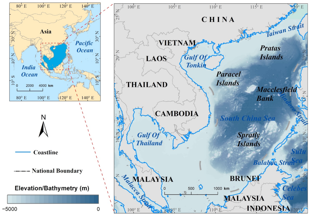
2.1. Study Area

The SCS is the second largest semi-enclosed sea in the world [8]. It is a vital sea-lane through which one-third of world trade passes, connecting with the East China Sea, the Western Pacific Ocean, the Java Sea, and the Indian Ocean through the Taiwan Strait, Bashi Strait, Karimata Strait and Malacca Strait respectively. Although the Gulf of Thailand is ecologically an isolated ecosystem, it is usually regarded as a part of the SCS. SCS has an area of 3.3 million km² excluding the Gulfs of Thailand and Tonkin, and up to 3.8 million km² of these gulfs are included [76]. Through plate tectonic evolution, diversified bottom topography with a strong contrast between margin and center has been configured in the SCS. The bottom topography ranges from the vast continental shelf (border of the continent), followed by steeped continental slopes, deep troughs and canyons, to the central basin (center of the SCS), with an average depth of 1212 m [77]. In the SCS, the shallower shelf fisheries occupy more than 80% of the total SCS catch because of the superior bio-hydrology conditions in the vast continental shelf. SCS spans across subtropical and tropical zones and is strongly influenced by ocean monsoonal climate. The prevailing climate feature in the SCS can be generally characterized by high temperature, moisture, precipitation and an apparent monsoon wind cycle throughout the year. Temperature distribution in the SCS is correlated with latitudinal zonality whereas spatio-temporal distribution of precipitation strongly depends on the regional monsoon climate. The winter monsoon season (November to March) is accompanied by a strong northeast wind and dry season. In contrast, the summer monsoon (May to August) is accompanied by a moderate southwest wind and humid season. Importantly, fishing-related mass and energy transportations such as salt, sediment, heat, and marine species, originating from the movement of surface current system (i.e., coastal currents, SCS Branch of Kuroshio Current and SCS Warm Current) [78] are also influenced by the monsoon. Furthermore, the coastline feature in the SCS is governed by monsoon and currents. In this study, the study area is defined between 3–23° N and 99–124° E, including the Gulf of Thailand and the Strait of Malacca, shown in Figure 2.

2.2. Dataset and Pre-Processing

The data used in this study include VIIRS DNB data and some relevant secondary data.

(1)

VIIRS DNB data. This study mainly relied on the version 1 monthly cloud-free VIIRS DNB composites from April 2012 to April 2019 provided by the Earth Observations Group (https://www.ngdc.noaa.gov/eog/viirs/download_dnb_composites.html (last accessed on 3 May 2021)). The VIIRS DNB data used in the study were monthly average radiance composite products excluding the data impacted by stray light, lightning, lunar illumination and cloud-cover, spanning from 75° N to 65° S. Each dataset contains average radiance images and cloud-free coverage. The monthly average radiance data has two configurations designated as ‘vcm’ and ‘vcmsl’ respectively. The ‘vcmsl’ version has reduced quality after the stray-light correction and its application is biased toward the poles. Thus, we selected the ‘vcm’ version (stray light-impacted data were excluded) for further analysis.

(2)

Administrative division data. The administrative division data used in this study, such as the national boundaries, coastlines and the range of islands and reefs were downloaded from the global administrative division website (http://www.gadm.org/version2 (last accessed on 3 May 2021)) at a scale of 1:1,000,000.

(3)

Gridded bathymetric datasets. Gridded bathymetric data used in this study were collected from the British Oceanographic Data Centre (BODC, http://www.bodc.ac.uk/data/online_delivery/gebco/ (last accessed on 3 May 2021)), which build global terrain models for ocean and land with a spatial resolution of 30 arc-second.

(4)

Tropical storm dataset. Tropical storm tracking information were collected from the digital typhoon website (http://agora.ex.nii.ac.jp/digital-typhoon/ (last accessed on 3 May 2021)). It provides a series of information for each labeled Northwest Pacific tropical cyclone at a six-hour interval from April 2012 to April 2019. A total 2363 records of tropical storms (wind speed > 17.2 m/s) in the SCS were selected for this study, which contains a list of key parameters such as name, duration(h), location (latitude and longitude), maximum wind speed(m/s) and influence radius.

(5)

Volunteer Observation Ship (VOS) data. VOS records are provided by the National Climatic Data Center (https://www.ncdc.noaa.gov/data-access/marineocean-data/vosclim/data-management-and-access (last accessed on 3 May 2021)) for reporting up-to-date information about the ship location and weather. Most ships recorded in the database were merchant ships in the world’s sea lane.

2.3. Methodology

In the SCS, the areas illuminated by human activity have notably higher radiance values in the VIIRS images than the background due to the ideal scenario of the dark ocean. Potential interference lights (e.g., lights from gas or oil platform, coastal or harbor, reef and islands, and merchant ship) will be masked out by using the false alarm mask factor. An examination of lit fishing vessel features in VIIRS images indicated that the radiance gradients between the object and its associated environment are much higher than those of the background. We have developed a set of algorithms for automatic detection of fishing activity and further investigated large-scale fishery dynamics in the SCS using monthly composite VIIRS DNB images between 2012 and 2019.

The following sections describe the analytical steps involved in this research: (1) preprocessing monthly images, (2) extracting false alarm mask factor, (3) detecting fishing vessels by integrating high gradient detection and a local adaptive thresholding, (4) investigating fishery dynamics using spatio-temporal analysis. The overall process is shown in Figure 3.

2.3.1. Pre-Processing

The VIIRS DNB images used for the nighttime fishing lights analysis were monthly average radiance composites. Prior to averaging, it had been filtered to exclude the data impacted by lightning, stray light, lunar illumination and cloud-cover. Temporal averaging can effectively reduce the potential interference by abrupt changes or noise. However, the difference between the object and background was artificially lessened by temporal averaging process, resulting in an omission of ship detection. Hence, prior to applying the VIIRS DNB images for NTL analysis, the VIIRS images were multiplied by the cloud-free observation images from the same month. Further, negative values, corresponding to non-light or typical background pixels were eliminated. Finally, the masked and fixed VIIRS images, and ancillary data were then standardized such as data normalization, project transformation, batch clip under clipping boundary of study area, and resampling.

2.3.2. False Alarm Mask Factor Extraction

In the VIIRS images, all non-zero pixels for potential non-fishing nighttime lights in monthly images were masked out by using the false alarm mask factor. In the SCS, the potential non-fishing nighttime lights were categorized into two groups: one is permanent sources whose locations remain stationary from one night to the next, including coastal or port, oil or gas platform flares, islands or reef and high-frequency nighttime activity; the other is a temporary source including merchant ships. Since existing databases were available for most non-fishing lights in this study, we compared to the existing database to control the possible contamination caused by non-fishing light sources.

(1)

Coastal light source: The light emissions from the coastal city or their port such as socio-economic activity and infrastructure construction fell within 2 km of the land set were labeled as coastal or port light source. The land-sea mask surrounded by a 2 km buffer is a basic mask for subsequent process.

(2)

Island/reef light source: The scattered islets in the SCS are either equipped with numerous illuminant facilities such as airports and lighthouses or not available for fishing. The nighttime lights set fell within 2 km of the islets dataset were labeled as island/reef light source.

(3)

Offshore oil/gas platform light source: The SCS possesses abundant oil/gas resource stock and frequent exploitation. In the VIIRS images, gas flares have notably higher brightness than the others. The offshore oil/gas set was defined by the known database of natural gas flares (1074 confirmed offshore platforms) in the SCS surrounded by a one km buffer accounting for the halo effect of gas flares.

(4)

High-frequency light source: The non-zero pixels for other potential permanent sources (e.g., lights from other platforms, storage boats or others unknown) were masked out by using NTL time series. The high-frequency source extent is recognized as pixels in an accumulated binary image during 2012–2019 that possess an occurrence frequency higher than a user-defined threshold (30) due to the spatio-temporal variability of fishing activity. The binary images were determined by using an empirical threshold 0.5 nW cm⁻² sr⁻¹ to remove the non-light pixels or noise.

(5)

Non-stationary ship light source (Merchant ship): The presence of numerous merchant ships in the SCS, as a vital sea-lane through which one-third of world trade passes, has significant consequence in the process of fishing vessels detection. All pixels for merchant ship lights were masked out by using the VOS-based mask. The VOS-based trajectory clustering analysis [79], including centerline of channel and trajectory extraction, was adopted to extract the merchant ship source mask.

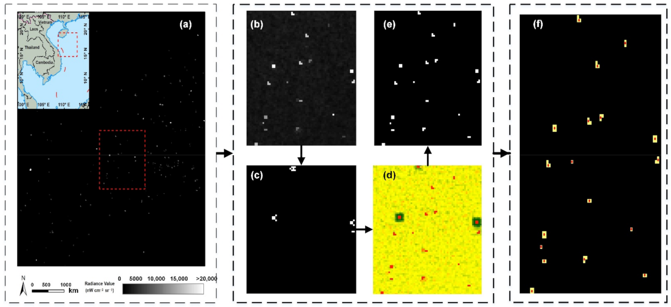
2.3.3. Detection Algorithms

Prior to ship detection, all non-zero pixels for potential interference light sources in monthly images were removed. False alarm mask factor extraction prepares the image for fishing vessel identification. Identifying areas illuminated by fishing lights in the VIIRS images is challenging because there is no direct relationship between fishing lights and NTL brightness. In the VIIRS images, the areas illuminated by the fishing vessels have notably higher radiance values than the background. However, a small portion of light-impacted background pixels can reach up to values around individual objects. In addition, intensified human activities are accompanied by fluctuations of surrounding environment and cross-impact among natural and anthropogenic nighttime light source, resulting in spatio-temporal fluctuations in brightness of background. The thresholding method, including histogram shape-based, clustering-based, entropy-based, object attribute-based, spatial and local methods, is a simplified method developed for differentiating object from the background and has been applied intensively in image segmentation analysis [80]. However, the application of direct thresholding in the SCS resulted in either omission or overestimation of the actual number of fishing lights because of the discreteness distribution present in the histogram. The previous study demonstrated that the intensity and luminance decrease away from the source with a Gaussian-like distribution [81]. The brightness or radiance gradients between object and its associated environment were confirmed to be much higher than those of the background. Accordingly, a new method was developed to integrate high gradient detection and adaptive local thresholding to better capture the location and brightness of fishing vessels in the SCS. The process of automatic detection consists of several phases: illumination edge detection, candidate detection, threshold detection and masking and vectorization, shown in Figure 4.

(1)

Illumination Edge Detection

Under clear viewing conditions, lit fishing vessels appear as either individual spots or loose clusters in the VIIRS DNB images. They occupy one to dozens of pixels and rank the most discernable pixels in the surrounding environments (e.g., light-impacted and non-light background) despite the spatio-temporal fluctuations in background brightness. More importantly, illuminance or intensity decreases away from the source with a Gaussian-like distribution [81]. Thus, we applied edge detection to detect and label high gradients in VIIRS DNB images. Edge detection is a computationally efficient gradient-based method developed for capturing structure feature without any prior knowledge and has been applied intensively in image segmentation. Edge, a collection of contiguous pixels with high gradients, can be used to differentiate the fishing lights from the light-impacted background. Edge detectors such as Laplacian-of-Gaussian (LOG), Sobel, Prewitt, Roberts, Canny were developed to boost the grouping correctness of edge pixels [82]. Canny algorithm was adopted to derive the accurate gradient images for further exploration because of its superiority in minutiae detection and locational accuracy. It can significantly suppress the spurious detections derived from false positives. Canny edge detection consisted of four substeps.

First, a 5 × 5 Gaussian filter was used to discard noise in the identified VIIRS images. Further, the radiance gradient calculation was computed at the pixel level by using Sobel operator to obtain gradient intensity/direction for each pixel. To eliminate spurious responses to the edge, we applied non-maximum suppression in the raw gradient results. Third, a double-threshold detection (high/low threshold) was adopted to screen out the true edge and construct contours. The optimal threshold determined by Otsu method has been widely chosen as the high threshold in the Canny algorithm because of its effectiveness and superiority in reducing false edges and improving locational accuracy. After processing a large number of images, we set 0.6 times the Otsu-derived optimal threshold as the high threshold and the low threshold was defined as 0.4 times high threshold. Accordingly, the pixels in monthly images were segmented into the potential edge and non-edge pixels by using determined low threshold. In the potential edge dataset, pixels that possess NTL gradient higher than the determined high threshold were assigned to strong edge points and were labeled as true edge points. The others were assigned to weak edge points. Then, tracing edge connection was run on each weak edge point. The weak edge point that possessed at least a strong edge in its eight neighbors was classified as the true edge.

(2)

Candidate Detection

Since the Canny-obtained edge data were available monthly in this study, the fishing vessels candidates could be inferred from the monthly radiance and edge images. According to the Gaussian-like distribution characteristics around the light source [81], the edge of illuminated areas were much lower than center points in radiance values. First, all non-zero pixels in the monthly binary edge images were replaced by NTL radiance values from the same month in monthly NTL radiance images. Further, a 5 × 5 average filter was adopted in the monthly edge radiance images to obtain the intensity and direction of radiance value in the neighborhood. Finally, the monthly difference images were created by subtracting the average filtered images from the monthly NTL radiance images processed in Section 2.3.2 from the same month. The difference images worked well for identifying the intensity and direction of pixels around the edge, especially for the light-impacted background. Thus, pixels that possessed higher values in the monthly difference images were recognized as fishing vessel candidates.

(3)

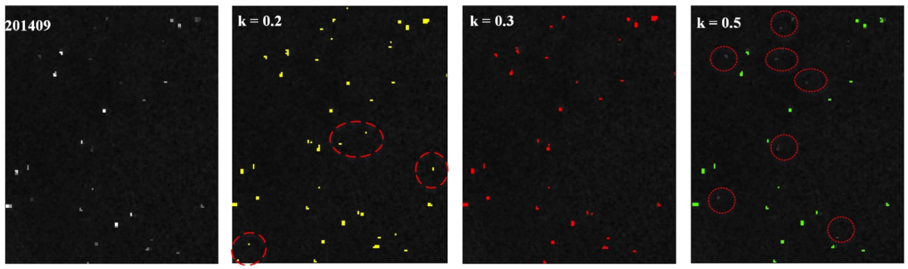
Threshold Detection

The monthly difference images were a de-noised and background-flattened version of spike image. In the monthly difference images, pixels having high values tend to be fishing vessel candidates. A thresholding method was adopted in the monthly difference image to segment the fishing vessels candidates from the background during 2012–2019. Considering the spatial heterogeneity, a local adaptive-threshold method was used in the monthly difference images to minimize possible omissions. Sauvola, a typical local thresholding, has superiority in processing changeable intensity of background caused by uneven lighting or complex background. The Sauvola algorithm performs on the gray image, and each threshold is determined by the local mean and standard deviation of all pixels’ gray value in the current pixel’s neighborhood. In this way, it can ideally differentiate the foreground from the background.

For a gray image, we assumed that the gray value of the current point (x,y) is g(x,y). In this section, pixels in the monthly difference image that possessed gray value higher than the threshold determined by Sauvola algorithm were classified as fishing vessels. The threshold can be calculated as:

$$\mathrm{t}\left(x,y\right)=m\left(x,y\right)·\left[1+k·\left(\frac{s\left(x,y\right)}{R}-1\right)\right]$$

(1)

where R is the dynamic range of the standard deviation (R = 128 for an 8 bit gray image), and k is a correction parameter (a user-defined constant) ranging from 0.2 to 0.5. m(x,y), s(x,y) are the mean and the local standard deviation computed in a window of s × s size centered on the current pixel. Equation (1) implies that Sauvola-obtained thresholds are determined adaptively by the local distribution and attribute values of pixels around the current pixel. Accordingly, it can meet our requirement for fishing vessel segmentation. In addition, Sauvola algorithm is a window-based local adaptive thresholding algorithm. In this study, k, an adjustable parameter, was used to adjust the accuracy of the segmentation and the window size is defined by local characteristic across the SCS. We set k as 0.3, and the window size as 50 pixels for all magnitudes of fishing activity by analyzing the distribution of fishing vessels sample values from visual identification and references for a better fitting. The Sauvola algorithm was tested in a typical densely distributed fishing activity sample with a dim contrast and different settings, shown in Figure 5. Figure 5 indicated that the best match between NTL-derived fishing vessels and visual identification from the same month occurred when k = 0.3 whereas the apparent omissions were in k = 0.5 and false positives were in k = 0.2, as shown in the red circles.

(4)

Masking and Vectorization

The Sauvola algorithm scanned the difference images and calculated the local threshold for each pixel. Threshold segmentation was applied in the difference images to segment the monthly images into fishing and non-fishing pixels. As such, the illuminated pixels ($\mathrm{difference}\mathrm{value}\ge \mathrm{threshold})$ were labeled as the corresponding light-fishing vessels. Additionally, binary images obtained from the Sauvola algorithm were used as a mask. We assumed that the (digital number (DN) > 0) values in the mask represented the real presence of fishing vessels. During the process, a pixel in a VIIRS radiance image, if its corresponding pixel in the mask was with value 1, the pixel value was preserved; otherwise, the pixel value was assigned 0. Finally, nighttime fishing boats dataset contains vector point dataset and raster dataset, and can report the location and brightness of nighttime lighting arising from nighttime fishing activity. The vector points dataset was obtained by converting the Sauvola-obtained binary images into polygons, followed by converting the polygons into points (i.e., the centroid of each polygon), shown in Figure 4e,f. Radiance images were obtained by replacing the non-zero values in the Sauvola-obtained binary images with VIIRS radiance images from the same month.

2.3.4. Time Series Analysis

Fishing light radiance signals, a non-stationary and non-linear series, varied both temporally and spatially. In this study, we selected the Hilbert-Huang transform (HHT), an adaptive time-frequency analysis, to investigate temporal fluctuations of fishing light. HHT decomposes the non-stationary time series into an ensemble of stationary components by adaptively sifting based on local characteristic [83] and has been applied in Satellite Image Time Series (SITS) analysis because of its high temporal resolution and effectiveness [84]. It consists of two steps: empirical mode decomposition (EMD) and Hilbert Spectral Analysis (HSA). First, EMD sequentially decomposes the non-linear and non-stationary signals into a finite number of Intrinsic Mode Functions (IMFs). Each IMF represents different mono oscillation mode based on inherent nature of the data. Further, Hilbert transform was applied to each EMD-obtained mono-component to obtain corresponding Hilbert spectrum for HSA. To improve the accuracy, Ensemble Empirical Mode Decomposition (EEMD) was developed for resolving the mode-mixing problem in EMD by adding Gaussian white noise to the original signals [85].

Considering the spatial heterogeneity, SCS was divided into equal-area grids with 0.5 degree. In this study, HHT algorithm was computed at the grid level. There are two steps in HHT algorithm for SITS analysis. First, we decomposed the fishing light radiance series into five IMFs and a residual by using EEMD algorithm (Equation (2)). EEMD is a noise-assisted data analysis, which adds a white Gaussian noise series to the original signals before EMD decomposition. EEMD regards the original signals and added white Gaussian noise series as a whole for decomposition and uses the ensemble means for each EEMD-obtained IMF as final result. An empirical noise amplitude 0.2 times the standard deviation of the original data with 100 trials was set in this study [84,85].

$$\mathrm{x}\left(\mathrm{t}\right)={\displaystyle \sum }_{j=1}^n{c}_j+r_n$$

(2)

The IMFs can be sequentially extracted from the original signals, ranging from high to low-frequency ones, corresponding to the different scales of fluctuation in the original signals. The final residual $r_n$ is the trend in the data.

HSA was then computed in each EEMD-obtained mono-component signal to obtain the Instantaneous Frequency (IF) and Hilbert spectrum for further analysis such as constructing seasonal/trend component. The average period for each IMF was obtained by the original length of the data divided by sum of IFs. We set the basic time unit and threshold to 12 months (one year) and 1.2 years, respectively. IMFs that met the aforementioned requirement were selected for constructing the seasonal component. The calculating result indicated that IMF1, IMF2, IMF3 and IMF5 satisfied the threshold. The IMF1 was previously verified to be closest to high-frequency noise [83,84,86]. Therefore, the IMF2, IMF3 and IMF5, or the sum of these IMFs were used for reconstructing the seasonal component. To directly depict the temporal pattern, seasonal energy, trend energy and their proportion to the original signal energy [86], trend slope and time cycle were computed at the grid level. The energy of fishing lights signal is the integral of squared amplitude, shown in Equation (3). The calculation method illustrated as follows:

$$E_0={\displaystyle \sum }_{i=1}^n{\left|x\left(i\right)\right|}^2$$

(3)

$$E_{season}={\displaystyle \sum }_k{\displaystyle \sum }_{j=1}^n{\left|IM{F}_k\left(j\right)\right|}^2\left(k=2,3,5\right)$$

(4)

$${\mathrm{E}}_{IMF1}={\displaystyle \sum }_{i=1}{\displaystyle \sum }_{j=1}^n{\left|IM{F}_i\left(j\right)\right|}^2$$

(5)

$$E_{trend}=E_0-E_{IMF1}-E_{season}$$

(6)

$$p_{season}=\frac{E_{season}}{E_0}\times 100\%$$

(7)

$$p_{trend}=\frac{E_{trend}}{E_0}\times 100\%$$

(8)

where n is the length of original signal in time scale, $E_0$, $E_{IMF1}$, $E_{season}$, $E_{trend}$ represent the energy of original fishing signals, noise component, seasonal component and trend component respectively. $p_{season}$ and $p_{trend}$ imply the energy proportion of seasonal and trend components in the original signals respectively.

3. Results

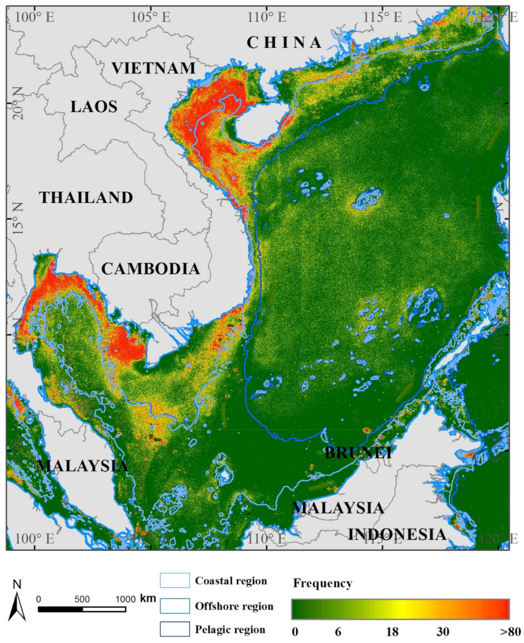
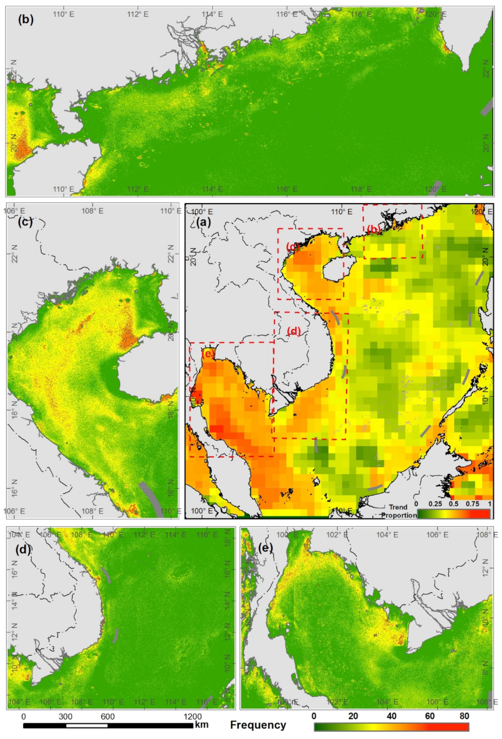
3.1. Spatial Analysis of Nighttime Fishing Lights in the SCS

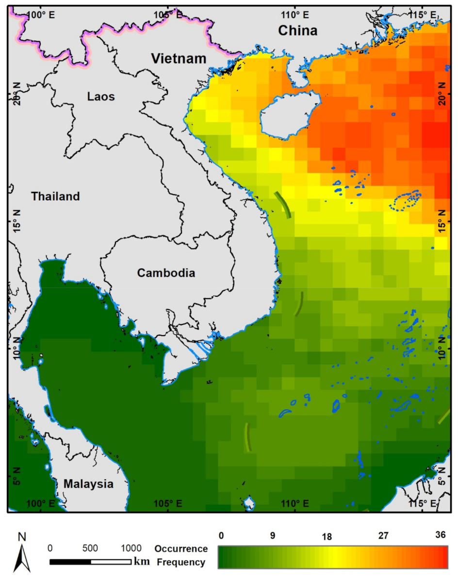
3.1.1. Distribution of Night-Time Fishing Lights in the SCS

Figure S1 presents the spatial distribution of fishing light points during 2012–2019 across the SCS. In general, a coastal-pelagic gradient of spatial distribution of fishing lights was observed, indicating a denser fishing activity in coastal or offshore than in pelagic regions. The coastal or offshore regions, especially the Gulfs of Tonkin and Thailand, experienced high fishing activity frequency during the period (Figure 6), and occupied a predominant role in fishing activity across the SCS. In contrast, only a small portion of fishing activity was detected in the deep sea.

In addition, spatial distribution of fishing activity varied strongly among the SCS countries. Specifically, fishing activity was mostly distributed on continental shelf and Gulf of Tonkin in the northern SCS for China. In the southern SCS, such as Cambodia and Thailand, most fishing activities occurred in Gulf of Thailand. For the western SCS, such as Vietnam, fishing activity concentrated in the Gulf of Thailand and eastern coast of Vietnam. Additionally, NTL-detected fishing activity was also observed in the western coast of the Philippines, northeastern Malay Peninsula and northwestern Kalimantan Island.

Monthly results indicated that NTL-detected fishing activity trajectories in the SCS during 2012–2019 could be categorized into three different cases: seasonal change, relatively stable condition and occasional disappearing/appearing (random distribution) (discussed in 3.1.2). Additionally, NTL-detected fishing light point dataset could be used to investigate the general trend (increase/decrease or stability) of fishing lights in a statistical sense during 2012–2019.

The numerical change of fishing lights in the SCS can be characterized by four stages over time: (1) a large rise stage when number of fishing lights increased sharply between end of winter (January or February) to spring (March to May), (2) a decline stage when number of fishing lights decreased sharply between end of spring (May) and summer, (3) a smaller rise stage when number of fishing lights increased gradually from end of summer (August) to autumn and (4) a smaller decline stage when number of fishing lights decreased gradually between end of autumn and winter. In summary, fishing activity in the SCS occurred consistently across the whole period with clear oscillations, and ranged from 29,389 to 105,942. Additionally, seasonal changes in number of fishing lights were evident in the SCS by using annually-averaged observations (Figure 7b). Generally, the number of fishing lights reached the maximum in spring (March) followed by a decline until the minimum in July. This trend was reversed from summer to winter. Moreover, the intensely-fished period concentrated in spring and autumn, accounting for 32% and 25% of the total annually-averaged number of nighttime fishing lights in the year. It should be noted that these numbers could underestimate the actual number of fishing vessels because of the nighttime fishing mode and the coarse resolution of VIIRS images.

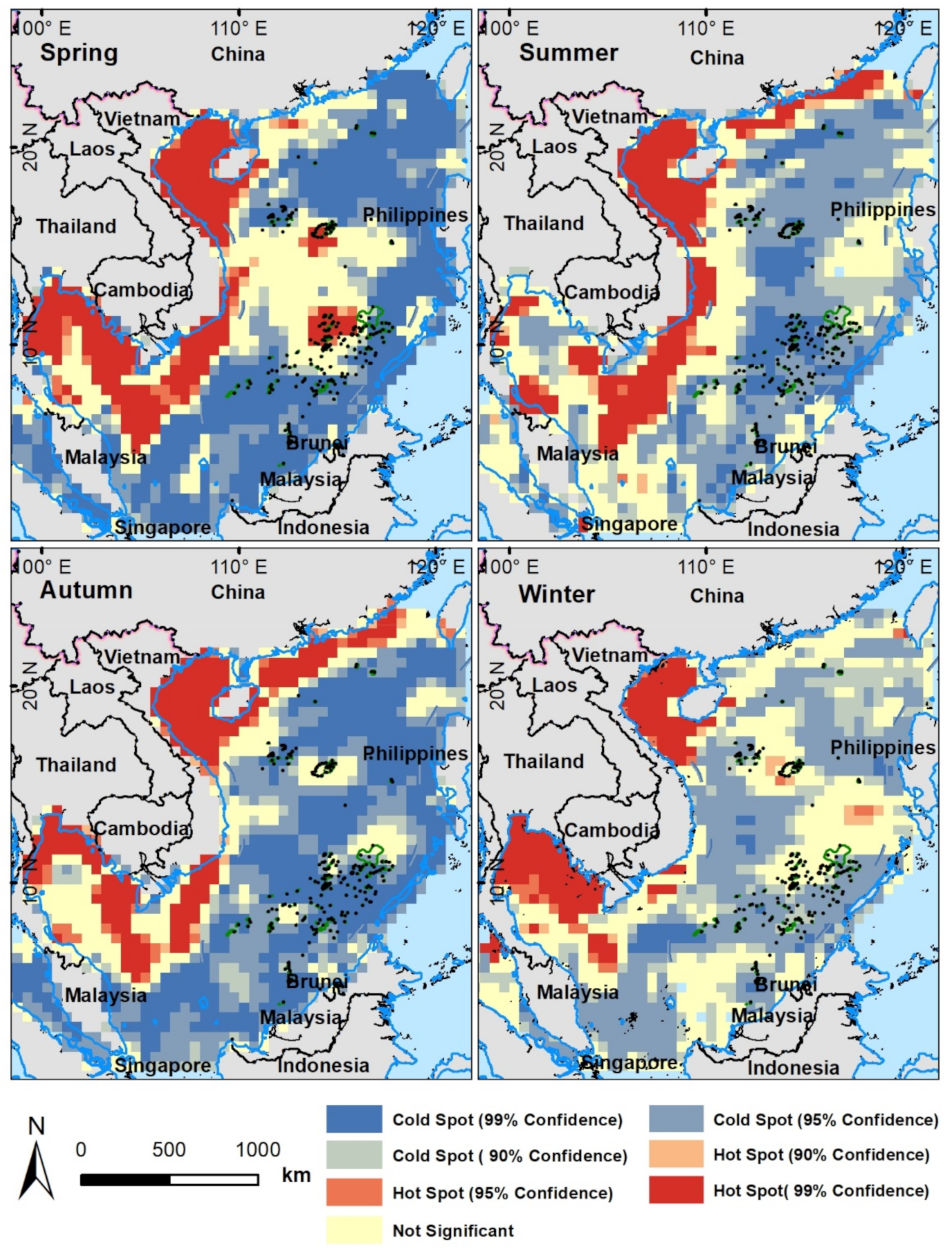
3.1.2. Spatial Getis-Ord Statistical Analysis

Figure 8 presents the detected hotspots, cold spots and random spots at a 0.5° grid level using Getis-Ord Gi* statistical analysis from 2012 to 2019. The number of each category and their proportion to the total grids were computed by using seasonal observations (

Table 1. The number of each category and their proportion to the total grids.

	Hotspots (p < 0.05)	Cold Spots (p < 0.05)	Random Spots
Spring	23.3%	45.7%	31%
Summer	23%	37%	40%
Autumn	21.3%	51.5%	27.2%
Winter	17.6%	35.2%	47.2%

). Compared to direct numerical analysis, the Gi*-derived results highlighted the actual spatial pattern of fishing activity while deemphasizing the occasional change. Most grids exhibited a statistically significant low-density or high-intensity spatial clustering. A shallow-pelagic divide was evident in the distribution of cold and hot spots. In addition to the seasonal high-density region in Macclesfield Bank and northern Spratly Islands, the east coast of the continent, especially in Gulfs (Gulfs of Tonkin and Thailand), showed significant high-density clustering. In contrast, the pelagic region and a small portion of the offshore region in southern SCS showed a significant low-density clustering.

Importantly, examination of per-grid Getis-Ord Gi* statistical analysis also provided important information on the intra-category change of fishing activity. The hot spot can be categorized by two groups. The spatial extent of hotspots remained overall stable across the whole period in Gulf of Tonkin. In contrast, an out-of-sync seasonal expansion or contraction in spatial extent of hotspots was detected among the others during the period. Specifically, sharp contractions were detected in summer and winter for Gulf of Thailand and eastern Vietnam, whereas an evident expansion was found in Pearl River during autumn.

Meanwhile, trajectories of cold spots in pelagic regions were characterized by three stages accompanied by seasonal contraction or expansion in spatial extent. First, cold spots shifted from marginal regions to inner regions with the extent contracted by 8.7%. Second, it expanded towards the surrounding regions with a peak in autumn and the extent increased by 14.5%. Further, the cold spots sharply shrank to the marginal region with the extent contracted by 16.3% and minimum in winter. However, an inverse trend was evident for random spots in pelagic region in both spatial extent and distribution, and the spatial extent of random spots reached its peak and trough in winter and autumn, respectively. Accordingly, fishing activity trajectories were categorized into three cases supported by Getis-Ord Gi* statistical analysis and seasonal analysis. The first one remained overall stable across the whole period with a slight contraction in certain times such as Gulf of Tonkin; the second case exhibited significant seasonality (e.g., seasonal contraction/expansion and seasonal migration) such as Gulf of Thailand, and a large portion of coastal and pelagic regions; another is an occasional case with a random distribution.

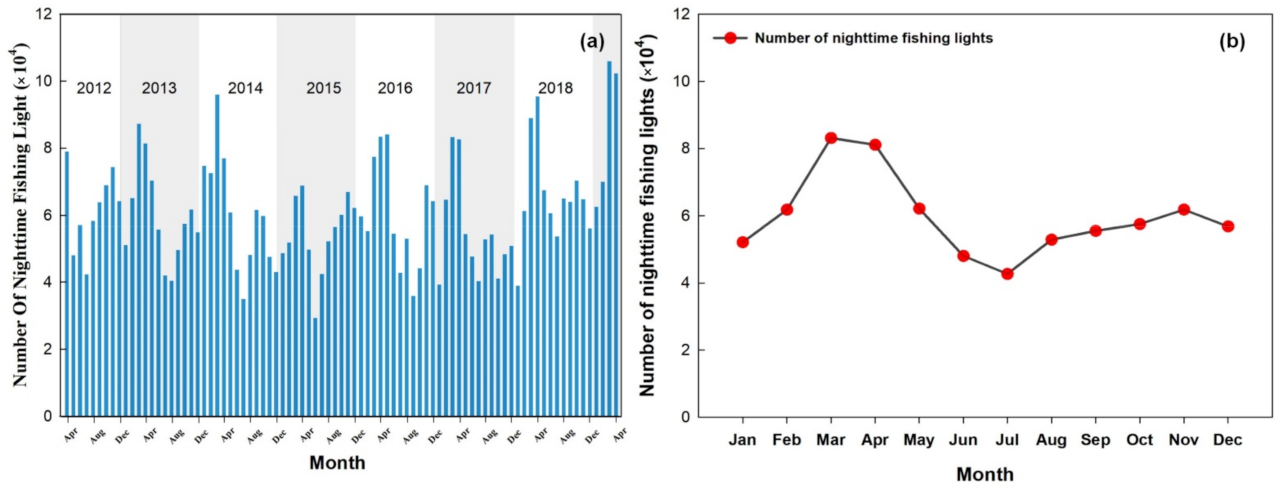
3.2. Temporal Series Analysis of Nighttime Fishing Activity

3.2.1. Time Frequency Analysis from HHT Transformation

The HHT-adjusted satellite image time series (SITS) analysis obtained an ensemble of disparate oscillation components ranked in descending order of time-frequency while de-emphasizing the abrupt change of NTL brightness. This was especially effective in constructing the seasonal and trend components in the SITS and providing an accurate portrait of dominant temporal pattern of fishing activity in the SCS during 2012–2019. Figure 9 presents detected distribution of seasonal and trend components during 2012–2019 using HHT time frequency analysis.

In general, an outward gradient of seasonal proportion was evident in the SCS with high values in deep sea followed by coastal or offshore regions, indicating a more obvious seasonal fluctuation in the pelagic regions than in coastal or offshore regions (Figure 9a). In addition to most pelagic regions, especially for northeastern and inner regions, the coastal region in southern China also showed relatively high seasonal proportions. In contrast, an inverse trend was observed for trend proportion, which indicated that NTL brightness in coastal regions, except for southern China, tended to be more stable than pelagic regions (Figure 9b). The trend proportion was generally high for most coastal and offshore regions, especially for Gulfs of Thailand and Tonkin, eastern and southern Vietnam. Further, a difference image was created by subtracting the seasonal proportion image from the trend proportion image to directly depict dominant temporal pattern at the grid level (Figure S2). In addition to northeastern and inner region in the deep sea, coastal-offshore regions in southern China and most pelagic regions also showed relatively high positive values, indicating a seasonality-dominant pattern of fishing activity in these regions. The result implied that fishing activity in these regions might occur during the fixed months of the year, with little or no fishing activity registered during the rest of the year. Low negative values in east coast of the continent, especially for joint region in Gulf of Tonkin, coast along Gulf of Thailand and east coast of Peninsular Malaysia implied that fishing activity in these regions tended to be more stable than in other regions. We interpret the relatively weak seasonality as indicating regions with small seasonal fluctuations hiding in the temporal pattern instead of non-seasonality. Combinedly, pixels or grids having a high trend proportion and simultaneously experiencing a high NTL brightness tend to be fishing agglomeration areas (discussed in Section 3.2.2). In summary, the seasonal-trend proportion has the capability to capture the most dominant temporal pattern of fishing activity in the SCS.

Further, the direction and change rate of trend, and annual cycle of seasonality in fishing activity were computed at the grid level. Trend slope is an annual-averaged change rate, explaining the change rate and direction (increasing/decreasing) of fishing activity during 2012–2019. A negative (positive) trend slope implies a decreasing (increasing) trend during 2012–2019 and a larger absolute value of trend slope indicates more rapid change than smaller values.

Most grids (63%) across the SCS, except for Gulf of Thailand and southern China, experienced an increasing trend during 2012–2019 and rapid growth was the regionally-dominant trend, as revealed by the average of 41.5. Specifically, the trend slope for most grids fell into the range of 0–200, with a few exceptions where the trend slope reached 400 in inner pelagic regions and as high as 2000 in Gulf of Tonkin (Figure 9d). In contrast, Gulf of Thailand and southern China, especially the Pearl River, exhibited a sharp decreasing trend, as revealed by the trend slope around −1500. In addition, trend slope can provide an accurate characterization of annual-averaged change for fishing activity at multiple scales (i.e., entire region, grid and subregion). A clear distinction was observed in four examples of subregions (i.e., Pearl River, Gulf of Tonkin, eastern Vietnam and Gulf of Thailand), representing different geography locations and variation characteristics. At the subregion level, the average trend slope ranged from 10 with 34% grids on the rise for eastern Vietnam to 385.2 with 71% grids on the rise for Gulf of Tonkin, indicating that the most rapid growth was in Gulf of Tonkin. Average trend slope in Gulf of Thailand (−5.64) and Pearl River (−55.3) echoed the strong decrease at the grid level.

Time period is a key element for describing intra-annual periodic fluctuations that have a regular cycle driven by diverse drivers such as annual climate conditions, seasonal regulations and socio-economic status. Figure 9c indicated that time cycles in the SCS varied spatially, and time cycle for most grids (90.8%) fell into the range of 0.6–1.1 years with a few exceptions in southern China, pelagic regions and Gulf of Thailand. The results indicated a significant seasonality of fishing activity with an overall time cycle of 0.79 years across the SCS.

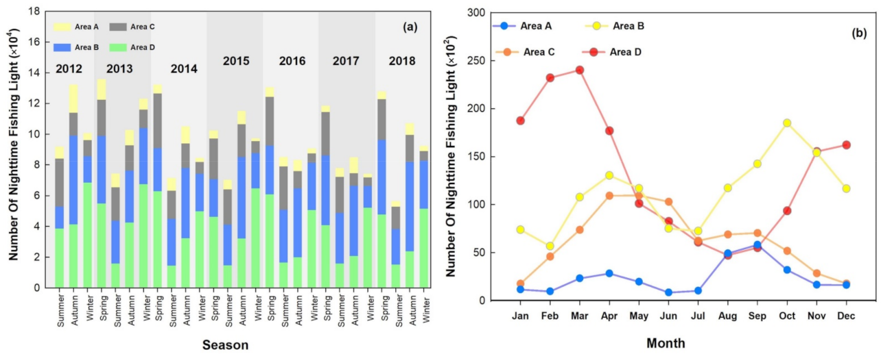
3.2.2. Temporal Analysis of Nighttime Fishing Light for Subregions

HHT-obtained results presented the most dominant temporal pattern of fishing activity during 2012–2019, revealed by seasonal and trend proportions, trend slope and time cycle, on the basis of the inherent nature of the SITS. From this point further, four HHT-derived representative subregions, were chosen as examples to provide an exhaustive characterization of local pattern of fishing activity in the SCS. As shown in Figure 10, area A is located around the Pearl River Estuary with a marked seasonality and a sharp decline; area B is in the Gulf of Tonkin with a high trend proportion and a rapid growth; area C is along the east coast of Vietnam with a high trend proportion; area D is in the Gulf of Thailand with a slight decline and a short time cycle. Specifically, subregion analysis was conducted in numerical and brightness dimensions. In this section, we conducted a numerical analysis at the subregion level.

Figure 11 presents the detected number of fishing lights during 2012–2019 for each subregion using monthly observations. The resulting patterns show apparent distinctions in temporal distributions of fishing lights among four subregions. In general, a similar and out-of-sync double-peak seasonal pattern was evident in subregions except for area D. Figure 11 shows that the large peak was in two autumn months (September and October) for areas A and B, whereas area C was the highest in May. The smaller peak for areas A and B occurred in April, and area C reached its smaller peak in September.

Specifically, fishing activity concentrated in autumn and spring in area A, accounting for 38% and 25% of the total number respectively. The larger drop during summer coincided with the Chinese fishery moratoria, and a smaller drop in winter corresponded to the Chinese New Year. Annual fishing moratorium has been actualized in the Chinese Exclusive Economic Zone (EEZ) since 1999, from May 16 (12:00 local time) to August 1 (12:00). It was adjusted from May 1 to August 16 after 2017.The impact of annual fishing moratorium is evident in area A, as revealed by the strong contrast in number of fishing lights between moratorium-on and moratorium-off periods. The minimum was detected in summer (June), much less than those in winter. The detected temporal pattern echoed the strong HHT-obtained seasonality in area A. The seasonal variation of number of fishing lights in area B generally follows a similar temporal pattern as that in area A. In contrast, the temporal distribution in area B was more balanced than area A among seasons, accounting for 26%, 20%, 36% and 18% of the total number respectively. Additionally, area B experienced much more fishing lights during the period, with the minimum reaching as high as 5753. It should be noted that area B was the lowest lighted in winter (February) instead of during summer because of the limited Chinese fishing moratorium coverage. In contrast with areas A and B, the number of fishing lights in area C gradually decreased among seasons, accounting for 39%, 31%, 20% and 11% of the total number respectively. In area D, the number of fishing lights remained overall relatively high with the largest amplitude. Seasonal variation in area D showed little coherence with others, peaking in very different seasons. Generally, the number of fishing lights reached the maximum in spring months (March) followed by a sharp decline until the minimum in August. This trend was reversed from autumn to spring. Additionally, fishing activity concentrated in winter and spring, accounting for 36.5% and 32.5% respectively whereas summer and autumn accounted for 12% and 19%. The annual change of number of fishing lights among subregions echoed the HHT-obtained trend slope. The temporal pattern among the subregions was supported by HHT analysis at the grid level.

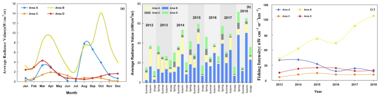
3.2.3. Temporal Analysis of Nighttime Fishing Intensity

VIIRS data cannot distinguish gear types and lighting types because of the sensor characteristics and the coarse resolution of VIIRS imagery. It should be noted that brightness is a synthetic indicator depending on intensity-related factors such as vessel size (e.g., gear type and vessel length) and light type/power. Accordingly, temporal change of fishing intensity can be revealed by the relative variation of brightness. In the VIIRS imagery, a higher NTL brightness indicates higher fishing intensity than smaller values. Hence, we aggregated the pixel-level NTL brightness to investigate temporal change of fishing intensity at different geographical scales. The accumulation radiance value, called the total of light radiance (TOL), represents the total fishing intensity at different geographical scales. Examination of TOL variation can provide an accurate characterization of temporal pattern of fishing intensity across the entire SCS. Generally, fishing intensity across the entire SCS can be characterized by the same four stages as that in number of fishing lights, except for the starting time of the fourth stage one month earlier (Figure 12). Additionally, a similar seasonal pattern of fishing intensity is evident across the SCS with the smaller peak one month earlier. Spring higher fishing intensity, accounted for 40% and 25% of the total fishing intensity respectively, whereas summer and winter accounted for 16.8% and 18.2% respectively.

From this point further, we explore the temporal pattern of local fishing intensity in the HHT-obtained four representative subregions. Because TOL depends on different geographical scales, we normalized the TOL by areas of each subregion to obtain a local indicator for further analysis. Specifically, area B consistently experienced much higher fishing intensity during the period, reaching as high as 9.37, followed by area A, then area D. In contrast, fishing intensity in area C was generally stable, with a slight oscillation around 0.89. Based on the aforementioned principle, area B was recognized as a fishing agglomeration area whereas area A tended to be a seasonal intensely-fished region with little or no fishing activity registered during summer. In addition, areas C and D were also relatively intensely-fished regions with medium fishing intensity.

The resulting patterns (Figure 13) show clear distinctions in temporal distributions of fishing intensity among four subregions, similar to that of number of fishing lights. A similar double-peak seasonal pattern was evident in subregions except for area D as that in number of fishing lights. The temporal pattern of fishing intensity among four subregions was consistent with that in number of fishing lights, with a few exceptions where both peaks in area A were one month earlier (August and April) and the large peak in area C was one month earlier (April). Specifically, autumn and spring experienced much higher fishing intensity for area A, accounting for 40% and 26% of total NTL intensity respectively. The weakest TOL during fishing moratorium and strong contrast in TOL between moratorium-on and moratorium-off period indicated that fishing moratorium was a main factor that impacted the TOL seasonality in area A. Additionally, the result implied the good compliance of regulation in area A. Hence, TOL can be an indicator to assess the compliance of regulation in restricted areas. In area B, temporal pattern of fishing intensity is similar to that of the number of fishing lights. Area B experienced much higher fishing intensity consistently during the period and had a relatively balanced temporal distribution among the seasons, accounting for 31%, 17%, 39% and 13% respectively. It reached the minimum in winter instead of summer because of the limited Chinese fishing moratorium coverage. Temporal pattern of fishing intensity in area C followed a similar decreasing trend among seasons as that in number of fishing lights. In area D, fishing activity was consistent throughout the year with a large amplitude. Fishing intensity peaked in spring (March) followed by a decline until the minimum in August. This trend was reversed from autumn to winter. Fishing intensity in spring and winter accounted for 41.5% and 33.7% of the total intensity, whereas low values were detected during summer and autumn. The fishing intensity in area D remained overall medium whereas fishing intensity during the large increase was slightly higher than that in area A during the same period (smaller increase). In addition, the annual change of fishing intensity among subregions can be categorized into three classes: stable (area C), sharp increasing trend (area B) and decreasing trend either sharp (area A) or gradual (area D) and was supported by the HHT-obtained trend slope at a subregion level.

4. Discussion

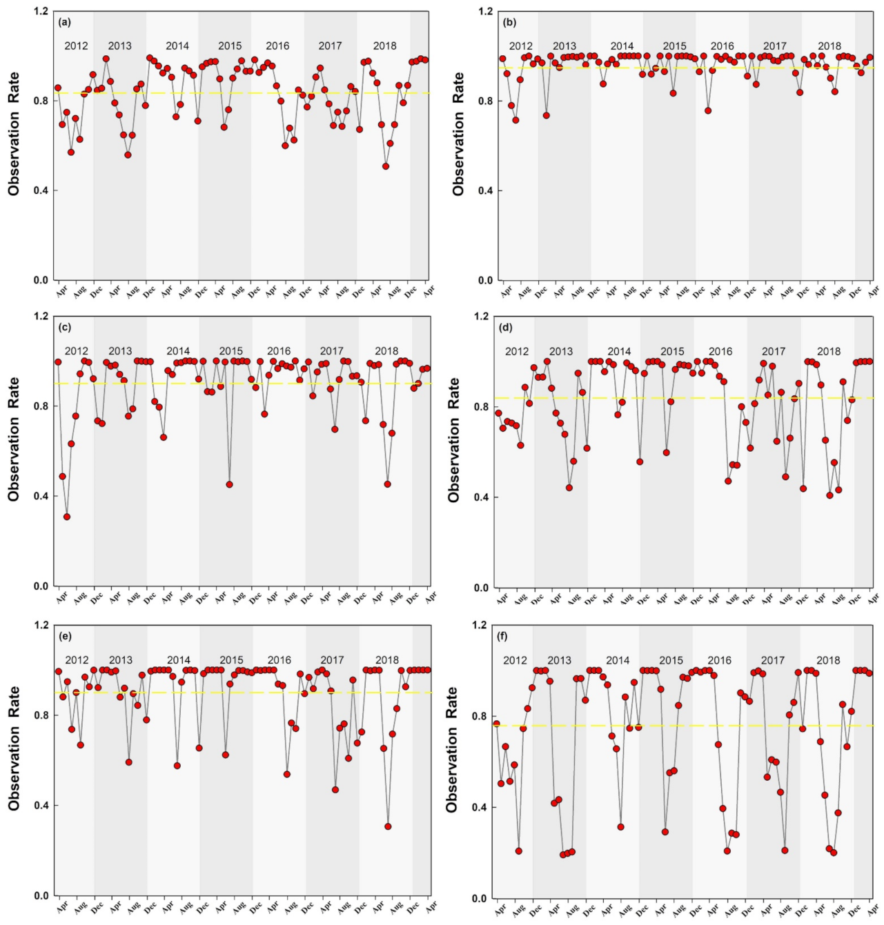
4.1. Impact of Cloud-Coverage

In this section, we evaluated the impacts of cloud coverage on NTL-based detection of fishery dynamics. The results can be used to evaluate the robustness of our experiment and diminish NTL variation caused by cloud-coverage. Pixels having at least two valid observations per month were classified as valid pixels. The number of valid pixels and its proportion to total pixel number (valid observation rate) were computed for six regions: entire SCS, the four above-mentioned subregions and pelagic areas in southern SCS respectively using all monthly cloud-free coverage observations.

Figure 14a indicated a good observation across the entire SCS with an overall accuracy of 0.84. The good valid observation rate confirmed the usefulness and robustness of the detected spatio-temporal pattern of fishing activity. In the five subregions, an average rate of 0.84 and 0.75 was obtained for area C (eastern Vietnam) and area D (Gulf of Thailand), whereas it reached 0.96 for area A, 0.9091 for area B and 0.90 for pelagic region in southern China. A slight cloud-coverage rate was obtained in areas A, B and pelagic region with cloud-impacted months smaller than 1%, 3.5% and 2.4% respectively, indicating a more accurate NTL-derived temporal pattern in these regions where the impact of cloud-cover can be ignored. It is noted that the cloud-impacted months reached 7.14% for area C and much higher for area D, where relatively high cloud coverage occurred during certain summer months. In area D, certain summer months provided the worst portrait of fishing activity in the SCS. Accordingly, a median filter was applied to the cloud-impacted radiance images in area C and D by adjusting cloud-impacted pixel values to the median of the three adjacent months in the corresponding locations. This strategy was used to diminish seasonal variation caused by cloud-coverage and enhance the robustness of our experimental results. Generally, the NTL images performed well in investigating fishery dynamics and conducting further analysis across the entire SCS, with a few exceptions where certain summer months in area D provided a worse characterization of fishing activity impacted by the cloud-coverage. The cloud-impacted images were replaced by the median value of the three adjacent months in the corresponding locations. Additionally, cloud-impacted images mostly occurred in low-latitude areas during summer and the valid observation rate gradually decreased as latitude went down.

4.2. Correlation Relationship between the TOL and the Number of Nighttime Fishing Light

The number of fishing lights and fishing intensity are crucial elements for fishing resource analysis. In the VIIRS images, a higher NTL brightness generally implies more fisheries catch than smaller values. In addition to the detected spatio-temporal pattern of the two elements, Pearson correlation coefficient was computed at the grid level between TOL and the number of nighttime fishing lights. The results can provide additional information on the distribution of SCS commercial fisheries resources. Since the analysis is based on the presence/absence of each variable to estimate the correlation, it is sensitive to the grid resolution, which alters the distribution of variables. A grid resolution of 0.5° was set after applying a set of grid resolutions in a large number of images.

$$\mathrm{r}=\frac{{{\displaystyle \sum }}_{i=1}^n\left(o_i-\overline{o}\right)\left(p_i-\overline{p}\right)}{\sqrt{{{\displaystyle \sum }}_{i=1}^n{\left(o_i-\overline{o}\right)}^2\times {{\displaystyle \sum }}_{i=1}^n{\left(p_i-\overline{p}\right)}^2}}$$

(9)

where $o_i$, $p_i$ are the monthly TOL and number of active fishing vessels in each grid during the observed period, $\overline{o}$ and $\overline{p}$ represent the annually-averaged TOL and the number of active fishing vessels in each grid.

In general, the spatial pattern of correlation coefficients showed a clear coastal-pelagic divide, shown in Figure 15. In addition to coast of the continent, the marginal region in deep sea also exhibited a strong correlation relationship, which can be explained by the intense fishing activity in these regions. The correlation coefficient ranged from 0.11 to 1 with an overall coefficient of 0.76 across the entire SCS. It indicated a moderate to strong correlation relationship between number of fishing lights and TOL for most grids with the weaker correlation proportion smaller than 5.1%. In addition to a small portion in Gulf of Tonkin and Pearl River Estuary, a large portion of pelagic regions exhibited relatively weaker correlation, especially in the deep sea. We interpret this weak relationship in the deep sea as indicating regions with either multiple fishing-related ocean-going vessel types such as cargo boats and trans-shipment vessels that our method cannot differentiate, or stable conditions that resulted from constrained conditions for fishing activity such as partial exposition of reef flats. The weaker correlation in waters around Pearl River Estuary and Gulf of Tonkin can be explained by saturation in fishing activity. In the four subregions, average correlation coefficient ranged from 0.78 (area B) to 0.86 (area C). Meanwhile, the strong correlation proportion were 76.7%, 47.2%, 83.1% and 66.9% respectively, indicating that a strong correlation relationship was evident among the four subregions and fish catch in area B could increase to be saturated.

4.3. The Impacts of Tropical Storms on the Nighttime Fishing Activity

The temporal pattern of fishing activity should be attributed to both environmental and anthropogenic factors. The dominant role of fishing moratorium in changing NTL brightness in the Chinese EEZ contributed to large NTL seasonality and the sharp decline during summer. Except for seasonal regulation, seasonal tropical cyclone activity in the SCS probably added to the seasonal variation of fishing-induced NTL brightness.

A synthetic indicator was developed to integrate the intensity, duration and influence areas to better indicate the tropical storm destruction potential:

$$E_i=I\times T\times \frac{S_i}{S_1}$$

(10)

$$\mathrm{ACE}={10}^{-4}\sum V_{max}{}^2$$

(11)

where $E_i$ and I are the destruction potential and the intensity of tropical storms activity for each time unit, T is the duration in the given region, S_i and S₁ are the storm-impacted areas and the total area. $V_{max}$ is the estimated maximum sustained velocity of each tropical storm.

In this study, I is described with the accumulated cyclone energy (ACE) by summing the squares of the maximum sustained wind speed (above 17.2 m/s) every six hours for all tropical cyclones over its lifetime in a tropical cyclone system, as shown in Equation (11). Interpretation model mentioned in [87] was used to build the hourly influence extent for further analysis. The model consisted of three steps: time point interpolation, node calculation and node connection.

Figure 16 presents the detected occurrence frequency of tropical storms during 2012–2019 in a 0.5° grid across the SCS (Figure 16). It is evident that the most cyclone-impacted region was in waters between Pratas Islands and Macclesfield Bank followed by southern China and Gulf of Tonkin, and then eastern Vietnam and waters between Macclesfield Bank and Spratly Islands. In the four subregions, an average cyclone-impacted frequency smaller than once a year was obtained for area C and D, whereas it reached 3.1 for area A and 2.27 for area B. To assess the impact of tropical storm activity on the fishing activity in the cyclone-impacted region, we adopted a Pearson correlation coefficient on a seasonal basis. The cyclone data using Equations (10) and (11) and interpretation model was conducted to derive seasonal destruction potential during 2012–2019 across the SCS.

Figure 17 indicates that tropical storms activity varied seasonally in areas A, B and the cyclone-impacted seasons were summer and autumn. It is noted that cyclone-impacted seasons partially coincided with the annual fishery moratorium in area A and the Chinese portion of area B. Accordingly, the Pearson correlation coefficient was computed in the time-series once the summer data was removed. It is evident that seasonal changes of fishing-induced NTL brightness were related to seasonal tropical storm activity in the SCS. A correlation coefficient of −0.9 was obtained for area A, and −0.83 for area B, indicating that periodical tropical storm activity strongly suppressed fishing activity in these regions, especially for area A. Although the relationship might be strengthened by incorporating additional drivers, fishing activity corresponds tightly to tropical storm activity.

5. Conclusions

Here we proposed an approach for automatic detection of nighttime fishing vessels and provided the first detailed large-scale dynamic analysis of nighttime fishing activity in SCS, using monthly composite VIIRS DNB images between 2012 and 2019. The proposed method effectively moderated the spatio-temporal fluctuations in radiance values of background and their implications to ship detection by integrating high radiance gradient detection and local adaptive thresholding. The trends of fishing activity in the SCS during 2012–2019 suggested a predominant role in coastal-offshore regions in numerical and intensity dimensions and a coastal-pelagic gradient of NTL seasonality. The detection of temporal change across the entire SCS indicated an overall increasing trend with an average trend slope of 41.5 and an increasing proportion of 63%, and the most rapid increasing/decrease in Pearl River and Gulf of Tonkin. In addition, NTL-detected fishing activity concentrated in spring and autumn except for the Gulf of Thailand. Nighttime fishing activity trajectories across the SCS were categorized into three cases: relatively stable (i.e., Gulf of Tonkin), seasonal change (i.e., Gulf of Thailand, a large portion of coastal and pelagic regions) and random distribution supported by Getis-Ord Gi* statistical and seasonal analysis. The fishing activity in four representative regions (i.e., Pearl River, Gulf of Tonkin, Eastern Vietnam and Gulf of Thailand) echoed the HHT-obtained general trend with inter-annual pattern ranging from the sharp decreasing to increasing. Subregion and correlation analysis suggested that four subregions tended to be fishing agglomeration areas and the Gulf of Tonkin could increase to be saturated. Our results highlighted spatio-temporal variability and heterogeneity of nighttime fishing activity in the SCS and indicated the key factors influencing the pattern, such as policy (e.g., holidays, annual Chinese fishery moratorium in the Chinese Exclusive Economic Zone (EEZ)) and natural factors (e.g., seasonal tropical storm activity).

Further, additional information such as field data, attribute data (i.e., types of lighting/boats and ownership of boats) can be incorporated with socio-economic information to provide a finer characterization of SCS marine fisheries. These data can become a powerful tool to enhance marine fisheries resources management, evaluate the effectiveness of existing governance regimes and accelerate the development of novel dynamic management approaches.

References

- McManus, J.W.; Shao, K.-T.; Lin, S.-Y. Toward establishing a Spratly Islands international marine peace park: Ecological importance and supportive collaborative activities with an emphasis on the role of Taiwan. Ocean. Dev. Int. Law 2010, 41, 270–280. [Google Scholar] [CrossRef]
- Paterson, C.J.; Pernetta, J.C.; Siraraksophon, S.; Kato, Y.; Barut, N.C.; Saikliang, P.; Vibol, O.; Chee, P.E.; Nguyen, T.T.N.; Perbowo, N.; et al. Fisheries refugia: A novel approach to integrating fisheries and habitat management in the context of small-scale fishing pressure. Ocean Coast. Manag. 2013, 85, 214–229. [Google Scholar] [CrossRef]
- Silvestre, G.; Garces, L.R.; Stobutzki, I.; Ahmed, M.; Valmonte-Santos, R.A.; Luna, C.Z.; Zhou, W. South and South-East Asian Coastal Fisheries: Their Status and Directions for Improved Management: Conference Synopsis and Recommendations. In WorldFish Center Conference Proceedings of Assessment, Management and Future Directions for Coastal Fisheries in Asian Countries, Penang, Malaysia; 2003; Volume 67, pp. 1–40. [Google Scholar]
- Teh, L.S.L.; Witter, A.; Cheung, W.W.L.; Sumaila, U.R.; Yin, X. What is at stake? Status and threats to South China Sea marine fisheries. Ambio 2017, 46, 57–72. [Google Scholar] [CrossRef] [PubMed] [Green Version]
- Zhang, J.; Zhang, K.; Chen, Z.; Dong, J.; Qiu, Y. Hydroacoustic studies on Katsuwonus pelamis and juvenile Thunnus albacares associated with light fish-aggregating devices in the South China Sea. Fish Res. 2021, 233, 105765. [Google Scholar] [CrossRef]
- Xu, L.; Wang, X.; Van Damme, K.; Huang, D.; Li, Y.; Wang, L.; Ning, J.; Du, F. Assessment of fish diversity in the South China Sea using DNA taxonomy. Fish Res. 2021, 233, 105771. [Google Scholar] [CrossRef]
- La Torre, G.L.; Cicero, N.; Bartolomeo, G.; Rando, R.; Vadalà, R.; Santini, A.; Durazzo, A.; Lucarini, M.; Dugo, G.; Salvo, A. Assessment and monitoring of fish quality from a coastal ecosystem under high anthropic pressure: A case study in southern Italy. Int. J. Environ. Res. Public Health 2020, 17, 3285. [Google Scholar] [CrossRef] [PubMed]
- Thang, N.D. Fisheries cooperation in the South China Sea and the (Ir)relevance of the sovereignty question. Asian J. Int. Law 2011, 2, 59. [Google Scholar] [CrossRef]
- Hal, R.; Griffioen, A.B.; Keeken, O.A. Changes in fish communities on a small spatial scale, an effect of increased habitat complexity by an offshore wind farm. Mar. Environ. Res. 2017, 126, 26–36. [Google Scholar] [CrossRef]
- Guan, W.; Gao, F.; Chen, X. Review of the applications of satellite remote sensing in the exploitation, management and protection of marine fisheries resources. J. Shanghai Ocean Univ. 2017, 26, 440–449. [Google Scholar] [CrossRef]
- Yu, W.; Chen, X.; Yi, Q.; Chen, Y. Spatio-temporal distributions and habitat hotspots of the winter–spring cohort of neon flying squid Ommastrephes bartramii in relation to oceanographic conditions in the Northwest Pacific Ocean. Fish Res. 2016, 175, 103–115. [Google Scholar] [CrossRef]
- Paulino, C.; Segura, M.; Chacón, G. Spatial variability of jumbo flying squid (Dosidicus gigas) fishery related to remotely sensed SST and chlorophyll-a concentration (2004–2012). Fish Res. 2016, 173, 122–127. [Google Scholar] [CrossRef]
- Solanki, H.U.; Bhatpuria, D.; Chauhan, P. Signature analysis of satellite derived SSHa, SST and chlorophyll concentration and their linkage with marine fishery resources. J. Mar. Syst. 2015, 150, 12–21. [Google Scholar] [CrossRef]
- Yasuda, T.; Ohshimo, S.; Yukami, R. Fishing ground hotspots reveal long-term variation in chub mackerel Scomber japonicus habitat in the East China Sea. Mar. Ecol. Prog. Ser. 2014, 501, 239–250. [Google Scholar] [CrossRef] [Green Version]
- Wang, W.; Zhou, C.; Shao, Q.; Mulla, D. Remote sensing of sea surface temperature and chlorophyll-a: Implications for squid fisheries in the north-west Pacific Ocean. Int. J. Remote Sens. 2010, 31, 4515–4530. [Google Scholar] [CrossRef]
- Kumari, B.; Raman, M. Whale shark habitat assessments in the northeastern Arabian Sea using satellite remote sensing. Int. J. Remote Sens. 2010, 31, 379–389. [Google Scholar] [CrossRef]
- Gauthier-Ouellet, M.; Dionne, M.; Ois, F.; King, T.; Bernatchez, L. Spatiotemporal dynamics of the Atlantic salmon (Salmo salar) Greenland fishery inferred from mixed-stock analysis. Can. J. Fish. Aquat. Sci. 2009, 66, 2040–2051. [Google Scholar] [CrossRef] [Green Version]
- Leeney, R.; Amies, R.; Broderick, A.; Witt, M.; Loveridge, J.; Doyle, J.; Godley, B. Spatio-temporal analysis of cetacean strandings and bycatch in a UK fisheries hotspot. Biodivers. Conserv. 2008, 17, 2323–2338. [Google Scholar] [CrossRef]
- Su, F.; Zhang, J.; Du, Y.; Zhou, C.; Shao, Q. Spatiotemporal variations of pelagic fishery resources in East China Sea. J. Nat. Resour. 2004, 19, 591–596. [Google Scholar] [CrossRef]
- Zhang, H.; Yang, S.-L.; Fan, W.; Shi, H.-M.; Yuan, S.-L. Spatial analysis of the fishing behaviour of Tuna Purse Seiners in the western and central Pacific based on vessel trajectory data. J. Mar. Sci. Eng. 2021, 9, 322. [Google Scholar] [CrossRef]
- Lin, Y.; Yu, X.; Huang, L.; Sanganyado, E.; Bi, R.; Li, P.; Liu, W. Risk assessment of potentially toxic elements accumulated in fish to Indo-Pacific humpback dolphins in the South China Sea. Sci. Total Environ. 2021, 761, 143256. [Google Scholar] [CrossRef]
- Zhang, K.; Guo, J.; Xu, Y.; Jiang, Y.; Fan, J.; Xu, S.; Chen, Z. Long-term variations in fish community structure under multiple stressors in a semi-closed marine ecosystem in the South China Sea. Sci. Total Environ. 2020, 745, 140892. [Google Scholar] [CrossRef] [PubMed]
- Wang, Y.; Yao, L.; Chen, P.; Yu, J.; Wu, Q.E. Environmental influence on the spatiotemporal variability of fishing grounds in the Beibu Gulf, South China Sea. J. Mar. Sci. Eng. 2020, 8, 957. [Google Scholar] [CrossRef]
- Zhang, M.; Wu, Y.; Qi, L.J.; Xu, M.Q.; Yang, C.H.; Wang, X.L. Impact of the migration behavior of mesopelagic fishes on the compositions of dissolved and particulate organic carbon on the northern slope of the South China Sea. Deep-Sea Res. Part II-Top. Stud. Oceanogr. 2019, 167, 46–54. [Google Scholar] [CrossRef]
- Wei, P.; Wang, X.; Ma, S.; Zhou, Y.; Huang, Y.; Su, Y.; Wu, Q.E. Analysis of current status of marine fishing in South China Sea. J. Shanghai Ocean Univ. 2019, 28, 976–982. [Google Scholar] [CrossRef]
- Wang, X.H.; Qiu, Y.S.; Du, F.Y.; Liu, W.D.; Sun, D.R.; Chen, X.; Yuan, W.W.; Chen, Y. Roles of fishing and climate change in long-term fish species succession and population dynamics in the outer Beibu Gulf, South China Sea. Acta Oceanol. Sin. 2019, 38, 1–8. [Google Scholar] [CrossRef]
- Su, L.; Chen, Z.; Zhang, P.; Li, J.; Wang, H.; Huang, J. Catch composition and spatial-temporal distribution of catch rate of light falling-net fishing in central and southern South China Sea fishing ground in 2017. South China Fish. Sci. 2018, 14, 11–20. [Google Scholar] [CrossRef]
- Chen, L.C.; Lan, K.W.; Chang, Y.; Chen, W.Y. Summer assemblages and biodiversity of larval fish associated with hydrography in the northern South China Sea. Mar. Coast. Fish. 2018, 10, 467–480. [Google Scholar] [CrossRef] [Green Version]
- Fan, J.; Chen, G.; Chen, Z. Forecasting fishing ground of calamary in the northern South China Sea according to habitat suitability index. South China Fish. Sci. 2017, 13, 11–16. [Google Scholar] [CrossRef]
- Asanuma, I.; Yamaguchi, T.; Park, J.; Mackin, K.; Mittleman, J. Detection of temporal change of fishery and island activities by DNB and SAR on the South China Sea. World Acad. Sci. Eng. Technol. Int. J. Comput. Electr. Autom. Control. Inf. Eng. 2017, 11, 252–255. [Google Scholar]
- Zheng, T.; Tang, Y. Analysis of current status of Chinese marine fishing fleet of South China Sea area. J. Shanghai Ocean Univ. 2016, 25, 620–627. [Google Scholar] [CrossRef]
- Zhang, L.; Li, Y.; Lin, L.; Yao, Z.; Yan, L.; Zhang, P. Fishery resources acoustic assessment of major economic species in south-central of the South China Sea. Mar. Fish. 2016, 38, 577–587. [Google Scholar] [CrossRef]
- Zhang, J.; Yao, Z.; Lin, L.; Li, Y.; Song, P.; Zhang, R.; Gao, T. Spatial distribution of biomass and fishery biology of main commercial fish in the mouth of Beibu bay and the southwestern waters of the Nansha Islands. Period. Ocean Univ. China 2016, 46, 158–167. [Google Scholar]
- Ji, S.; Zhou, W.; Wang, L.; Tang, F.; Wu, Z.; Chen, G. Relationship between temporal-spatial distribution of yellowfin tuna (Thunnus albacares) fishing grounds and sea surface temperature in the South China Sea and adjacent waters. Mar. Fish. 2016, 38, 9–16. [Google Scholar] [CrossRef]
- Yan, L.; Zhang, P.; Yang, L.; Yang, B.; Tan, Y.; Chen, S. A study of sinking characteristics of light falling-net fishing in the South China Sea. J. Shanghai Ocean Univ. 2014, 23, 146–153. [Google Scholar]
- Zhang, P.; Zeng, X.; Yang, L.; Peng, C.; Zhang, X.; Yang, S.; Tan, Y.; Yang, B.; Yan, L. Analyses on fishing ground and catch composition of large-scale light falling-net fisheries in South China Sea. South China Fish. Sci. 2013, 9, 74–79. [Google Scholar]
- Daqamseh, S.T.; Mansor, S.; Pradhan, B.; Billa, L.; Mahmud, A.R. Potential fish habitat mapping using MODIS-derived sea surface salinity, temperature and chlorophyll-a data: South China Sea Coastal areas, Malaysia. Geocarto Int. 2013, 28, 546–560. [Google Scholar] [CrossRef]
- Wang, X.; Qiu, Y.; Du, F.; Lin, Z.; Sun, D.; Huang, S. Dynamics of demersal fish species diversity and biomass of dominant species in autumn in the Beibu Gulf, northwestern South China Sea. Acta Ecol. Sin. 2012, 32, 333–342. [Google Scholar] [CrossRef] [Green Version]
- Chen, G.; Li, Y.; Chen, P.; Zhang, J.; Fang, L.; Li, N. Measurement of single-fish target strength in the South China Sea. Chin. J. Oceanol. Limnol. 2012, 30, 554–562. [Google Scholar] [CrossRef]
- Guiet, J.; Galbraith, E.; Kroodsma, D.; Worm, B. Seasonal variability in global industrial fishing effort. PLoS ONE 2019, 14, e0216819. [Google Scholar] [CrossRef] [PubMed]
- Kroodsma, D.A.; Mayorga, J.; Hochberg, T.; Miller, N.A.; Boerder, K.; Ferretti, F.; Wilson, A.; Bergman, B.; White, T.D.; Block, B.A. Tracking the global footprint of fisheries. Science 2018, 359, 904–908. [Google Scholar] [CrossRef] [PubMed] [Green Version]
- Bharti, N.; Tatem, A.J.; Ferrari, M.J.; Grais, R.F.; Djibo, A.; Grenfell, B.T. Explaining seasonal fluctuations of measles in Niger using nighttime lights imagery. Science 2011, 334, 1424–1427. [Google Scholar] [CrossRef] [Green Version]
- Cao, X.; Chen, J.; Imura, H.; Higashi, O. A SVM-based method to extract urban areas from DMSP-OLS and SPOT VGT data. Remote Sens. Environ. 2009, 113, 2205–2209. [Google Scholar] [CrossRef]
- Croft, T.A. The Brightness of Lights on Earth at Night, Digitally Recorded by DMSP Satellite; U.S. Geological Survey: Reston, VA, USA, 1979; p. 66. [Google Scholar]
- Dwyer, R.G.; Bearhop, S.; Campbell, H.A.; Bryant, D.M. Shedding light on light: Benefits of anthropogenic illumination to a nocturnally foraging shorebird. J. Anim. Ecol. 2013, 82, 478–485. [Google Scholar] [CrossRef] [PubMed]
- Elvidge, C.; Ziskin, D.; Baugh, K.; Tuttle, B.; Ghosh, T.; Pack, D.; Erwin, E.; Zhizhin, M. A fifteen year record of global natural gas flaring derived from satellite data. Energies 2009, 2, 595–622. [Google Scholar] [CrossRef]
- Elvidge, C.D.; Baugh, K.E.; Kihn, E.A.; Kroehl, H.W.; Davis, E.R.; Davis, C.W. Relation between satellite observed visible-near infrared emissions, population, economic activity and electric power consumption. Int. J. Remote Sens. 1997, 18, 1373–1379. [Google Scholar] [CrossRef]
- Imhoff, M.L.; Lawrence, W.T.; Elvidge, C.D.; Paul, T.; Levine, E.; Privalsky, M.V.; Brown, V. Using nighttime DMSP/OLS images of city lights to estimate the impact of urban land use on soil resources in the United States. Remote Sens. Environ. 1997, 59, 105–117. [Google Scholar] [CrossRef]
- Kuechly, H.U.; Kyba, C.C.; Ruhtz, T.; Lindemann, C.; Wolter, C.; Fischer, J.; Hölker, F. Aerial survey and spatial analysis of sources of light pollution in Berlin, Germany. Remote Sens. Environ. 2012, 126, 39–50. [Google Scholar] [CrossRef]
- Ma, T.; Zhou, Y.; Zhou, C.; Haynie, S.; Pei, T.; Xu, T. Night-time light derived estimation of spatio-temporal characteristics of urbanization dynamics using DMSP/OLS satellite data. Remote Sens. Environ. 2015, 158, 453–464. [Google Scholar] [CrossRef]
- Mazor, T.; Levin, N.; Possingham, H.P.; Levy, Y.; Rocchini, D.; Richardson, A.J.; Kark, S. Can satellite-based night lights be used for conservation? The case of nesting sea turtles in the Mediterranean. Biol. Conserv. 2013, 159, 63–72. [Google Scholar] [CrossRef] [Green Version]
- Rodrigues, P.; Aubrecht, C.; Gil, A.; Longcore, T.; Elvidge, C. Remote sensing to map influence of light pollution on Cory’s shearwater in São Miguel Island, Azores Archipelago. Eur. J. Wildl. Res. 2012, 58, 147–155. [Google Scholar] [CrossRef]
- Small, C.; Pozzi, F.; Elvidge, C.D. Spatial analysis of global urban extent from DMSP-OLS night lights. Remote Sens. Environ. 2005, 96, 277–291. [Google Scholar] [CrossRef]
- Waluda, C.; Yamashiro, C.; Elvidge, C.; Hobson, V.; Rodhouse, P. Quantifying light-fishing for Dosidicus gigas in the eastern Pacific using satellite remote sensing. Remote Sens. Environ. 2004, 91, 129–133. [Google Scholar] [CrossRef]
- Yi, K.; Tani, H.; Li, Q.; Zhang, J.; Guo, M.; Bao, Y.; Wang, X.; Li, J. Mapping and evaluating the urbanization process in northeast China using DMSP/OLS nighttime light data. Sensors 2014, 14, 3207–3226. [Google Scholar] [CrossRef] [PubMed] [Green Version]
- Zhang, Q.; Seto, K.C. Mapping urbanization dynamics at regional and global scales using multi-temporal DMSP/OLS nighttime light data. Remote Sens. Environ. 2011, 115, 2320–2329. [Google Scholar] [CrossRef]
- Yu, B.; Deng, S.; Liu, G.; Yang, C.; Chen, Z.; Hill, C.J.; Wu, J. Nighttime light images reveal spatial-temporal dynamics of global anthropogenic resources accumulation above ground. Environ. Sci. Technol. 2018, 52, 11520–11527. [Google Scholar] [CrossRef] [PubMed] [Green Version]
- Li, D.; Li, X. An overview on data mining of nighttime light remote sensing. Acta Geod. Cartogr. Sin. 2015, 44, 591–601. [Google Scholar] [CrossRef]
- Levin, N.; Kyba, C.C.M.; Zhang, Q.; Sánchez de Miguel, A.; Román, M.O.; Li, X.; Portnov, B.A.; Molthan, A.L.; Jechow, A.; Miller, S.D.; et al. Remote sensing of night lights: A review and an outlook for the future. Remote Sens. Environ. 2020, 237, 111443. [Google Scholar] [CrossRef]
- Xu, Z.; Xu, Y. Study on the spatio-temporal evolution of the Yangtze River Delta urban agglomerationby integrating DMSP/OLS and NPP/VIIRS Nighttime Light Data. J. Geo-Inf. Sci. 2021, 23, 837–849. [Google Scholar] [CrossRef]
- Waluda, C.M.; Griffiths, H.J.; Rodhouse, P.G. Remotely sensed spatial dynamics of the Illex argentinus fishery, Southwest Atlantic. Fish Res. 2008, 91, 196–202. [Google Scholar] [CrossRef]
- Kiyofuji, H.; Saitoh, S.-I. Use of nighttime visible images to detect Japanese common squid Todarodes pacificus fishing areas and potential migration routes in the Sea of Japan. Mar. Ecol.-Prog. Ser. 2004, 276, 173–186. [Google Scholar] [CrossRef]
- Cho, K.; Ito, R.; Shimoda, H.; Sakata, T. Technical note and cover fishing fleet lights and sea surface temperature distribution observed by DMSP/OLS sensor. Int. J. Remote Sens. 1999, 20, 3–9. [Google Scholar] [CrossRef]
- Elvidge, C.D.; Baugh, K.E.; Zhizhin, M.; Hsu, F.-C. Why VIIRS data are superior to DMSP for mapping nighttime lights. Proc. Asia-Pac. Adv. Netw. 2013, 35, 62–69. [Google Scholar] [CrossRef] [Green Version]
- Liang, C.K.; Mills, S.; Hauss, B.I.; Miller, S.D. Improved VIIRS day/night band imagery with near-constant contrast. IEEE Trans. Geosci. Remote Sens. 2014, 52, 6964–6971. [Google Scholar] [CrossRef]
- Miller, S.D.; Turner, R.E. A dynamic lunar spectral irradiance data set for NPOESS/VIIRS day/night band nighttime environmental applications. IEEE Trans. Geosci. Remote Sens. 2009, 47, 2316–2329. [Google Scholar] [CrossRef]
- Li, X.; Ma, R.; Zhang, Q.; Li, D.; Liu, S.; He, T.; Zhao, L. Anisotropic characteristic of artificial light at night—Systematic investigation with VIIRS DNB multi-temporal observations. Remote Sens. Environ. 2019, 233, 111357. [Google Scholar] [CrossRef]
- Straka, W.; Seaman, C.; Baugh, K.; Cole, K.; Stevens, E.; Miller, S. Utilization of the suomi national polar-orbiting partnership (NPP) visible infrared imaging radiometer suite (VIIRS) day/night band for arctic ship tracking and fisheries management. Remote Sens. 2015, 7, 971–989. [Google Scholar] [CrossRef] [Green Version]
- Kyba, C.; Garz, S.; Kuechly, H.; de Miguel, A.; Zamorano, J.; Fischer, J.; Hölker, F. High-resolution imagery of earth at night: New sources, opportunities and challenges. Remote Sens. 2015, 7, 1–23. [Google Scholar] [CrossRef] [Green Version]
- Liu, Y.; Saitoh, S.-I.; Hirawake, T. Detection of squid and pacific saury fishing vessels around Japan using VIIRS day/night band image. Proc. Asia-Pac. Adv. Netw. 2015, 39, 28–39. [Google Scholar] [CrossRef]
- Zhang, X.; Saitoh, S.-I.; Hirawake, T.; Nakada, S.; Koyamada, K.; Awaji, T.; Ishikawa, Y.; Igarashi, H. An Attempt of Dissemination of Potential Fishing Zones Prediction Map of Japanese Common Squid in the Coastal Water, Southwestern Hokkaido, Japan. In Proceedings of the Asia-Pacific Advanced Network, A-Ju Art Gallery, Daejeon, Korea, 20–21 August 2013; pp. 132–141. [Google Scholar]
- Elvidge, C.; Zhizhin, M.; Baugh, K.; Hsu, F.-C. Automatic boat identification system for VIIRS low light imaging data. Remote Sens. 2015, 7, 3020–3036. [Google Scholar] [CrossRef] [Green Version]
- Cozzolino, E.; Lasta, C.A. Use of VIIRS DNB satellite images to detect jigger ships involved in the Illex argentinus fishery. Remote Sens. Appl. Soc. Environ. 2016, 4, 167–178. [Google Scholar] [CrossRef]
- Lebona, B.; Kleynhans, W.; Celik, T.; Mdakane, L. Ship Detection Using VIIRS Sensor Specific Data. In Proceedings of the IEEE International Geoscience and Remote Sensing Symposium (IGARSS), Beijing, China, 10–15 July 2016; pp. 1245–1247. [Google Scholar]
- Yamaguchi, T.; Asanuma, I.; Park, J.G.; Mackin, K.J.; Mittleman, J. Estimation of Vessel Traffic Density from Suomi NPP VIIRS Day/Night Band. In Proceedings of the Oceans Mts/Ieee Monterey, Monterey, CA, USA, 19–23 September 2016; pp. 1–5. [Google Scholar]
- Morton, B.; Blackmore, G. South China Sea. Mar. Pollut. Bull. 2001, 42, 1236–1263. [Google Scholar] [CrossRef]
- Liu, Z.F.; Zhao, Y.L.; Colin, C.; Stattegger, K.; Wiesner, M.G.; Huh, C.A.; Zhang, Y.W.; Li, X.J.; Sompongchaiyakul, P.; You, C.F.; et al. Source-to-sink transport processes of fluvial sediments in the South China Sea. Earth-Sci. Rev. 2016, 153, 238–273. [Google Scholar] [CrossRef]
- Alford, M.H.; Peacock, T.; MacKinnon, J.A.; Nash, J.D.; Buijsman, M.C.; Centurioni, L.R.; Chao, S.-Y.; Chang, M.-H.; Farmer, D.M.; Fringer, O.B.J.N. The formation and fate of internal waves in the South China Sea. Nature 2015, 521, 65–69. [Google Scholar] [CrossRef] [PubMed]
- Wang, J.; Li, M.; Liu, Y.; Zhang, H.; Zou, W.; Cheng, L. Safety assessment of shipping routes in the South China Sea based on the fuzzy analytic hierarchy process. Saf. Sci. 2014, 62, 46–57. [Google Scholar] [CrossRef]
- Sezgin, M.; Sankur, B. Survey over image thresholding techniques and quantitative performance evaluation. J. Electron. Imaging 2004, 13, 146–168. [Google Scholar] [CrossRef]
- Cao, C.; Bai, Y. Quantitative analysis of VIIRS DNB nightlight point source for light power estimation and stability monitoring. Remote Sens. 2014, 6, 11915–11935. [Google Scholar] [CrossRef] [Green Version]
- Canny, J. A computational approach to edge detection. IEEE Trans. Pattern Anal. Mach. Intell. 1986, 8, 679–698. [Google Scholar] [CrossRef]
- Wu, Z.; Huang, N.E.; Long, S.R.; Peng, C. On the trend, detrending, and variability of nonlinear and nonstationary time series. Proc. Natl. Acad. Sci. USA 2007, 104, 14889–14894. [Google Scholar] [CrossRef] [Green Version]
- Kong, Y.; Meng, Y.; Li, W.; Yue, A.; Yuan, Y. Satellite image time series decomposition based on EEMD. Remote Sens. 2015, 7, 15583–15604. [Google Scholar] [CrossRef] [Green Version]
- Wu, Z.; Huang, N.E. Ensemble empirical mode decomposition: A noise-assisted data analysis method. Adv. Adapt. Data Anal. 2009, 1, 1–41. [Google Scholar] [CrossRef]
- Xia, Z.; Li, D.; Li, X.; Zhao, L.; Wu, C. Spatial and seasonal patterns of night-time lights in global ocean derived from VIIRS DNB images. Int. J. Remote Sens. 2018, 39, 8151–8181. [Google Scholar] [CrossRef]
- Sun, C.; Liu, Y.; Li, M.; Chen, Z.; Zhao, S. An analysis of tropical storms impact on islands and reefs in the South China Sea in the past 35 years. Remote Sens. Land Resour. 2014, 26, 135–140. [Google Scholar] [CrossRef]