Station-Keeping Control of Autonomous and Remotely-Operated Vehicles for Free Floating Manipulation

Abstract

This paper investigates the station-keeping control of autonomous and remotely-operated vehicles (ARVs) for free-floating manipulation under model uncertainties and external disturbances. A modified adaptive generalized super-twisting algorithm (AGSTA) enhanced by adaptive tracking differentiator (ATD) and reduced-order extended state observer (RESO) is proposed. The ATD is used to obtain the smooth reference signal and its derivative. The RESO is used to estimate and compensate for the model uncertainties and external disturbances in real-time, which enhances the robustness of the controller. The modified AGSTA ensures the fast convergence of the system states and maintains them in a predefined neighborhood of origin without overestimating control gains. Besides, the proposed new variable gain strategy completely avoids the control gains vibrating near the set minimum value. Thanks to the RESO, the proposed controller is model-free and can be easily implemented in practice. The stability of the closed-loop system is analyzed based on Lyapunov’s direct method in the time domain. Finally, the proposed control scheme is applied to the station-keeping control of Haidou-1 ARV, and the simulation results confirm the superiority of the proposed control scheme over the original AGSTA.

1. Introduction

In recent years, unmanned underwater vehicles (UUVs) have been widely utilized in various areas such as marine science, marine rescue, and offshore industry [1]. A considerable number of these applications require UUVs have intervention capabilities. Currently, most intervention tasks are faced up by a remotely operated vehicle (ROV) equipped with one or multiple manipulators. However, the ROV needs to be controlled by highly skilled operators via a master-slave approach, which increases human fatigue over time and has a more significant time delay in the control loop [2]. Furthermore, the ROV requires an expensive support vessel equipped with dynamic positioning (DP) systems and capable of handling the umbilical cable. As a result, the ROV can only work in a small zone due to the umbilical cable’s restriction. To overcome these limitations, ARV has been proposed for deep-sea exploration and intervention. The ARV communicates with the support vessel through an optical fiber instead of an umbilical cable. Thus, the ARV can deploy and operate from vessels lacking DP capabilities, which reduces operational costs [3]. The main features of the ARV lie in that it can perform large-scale exploration tasks, monitoring tasks, and underwater intervention tasks in different operational modes.

The ARV we investigate in this paper is called Haidou-1. It is composed of a fully-actuated vehicle and a six DoFs deep-sea electric manipulator, as shown in Figure 1. It should note that Haidou-1 is a typical underwater vehicle manipulator system (UVMS). Thus, the research on UVMS can also be applied to our research. When the Haidou-1 performs free-floating manipulation, such as seabed sampling, it will be desired that the vehicle has a station-keeping function (the vehicle’s ability to maintain the same position and attitude at all times even under disturbances). However, in order to achieve stability and maneuverability simultaneously, the metacentric height of the ARV is set lower than that of a conventional ROV. Besides, the ARV thrusters’ performance is weaker than the traditional ROV. Therefore, the dynamic coupling effect caused by the motion of the manipulator has a substantial impact on the vehicle. The vehicle will deviate from the desired position and attitude, thereby severely reducing the accuracy of the manipulator’s end-effector. Therefore, the station-keeping control of the vehicle is essential for free-floating manipulation. However, the design of the controller is quite challenging work due to the coupling effects, strong nonlinearity, random external disturbances, unpredicted ocean currents, and the difficulty in accurately modeling the hydrodynamic effects [4].

There exist two main strategies for UVMS control in the literature. The first strategy controls the whole system at the operational space level, treating the UVMS as a single system [5,6,7]. Another strategy aims to decouple the UVMS and independently control the vehicle and the manipulator [8]. When the vehicle and manipulator have similar dynamic characteristics or bandwidth, the first strategy is feasible. However, Haidou-1 has a big difference in vehicle and manipulator inertias. Moreover, the UVMS as a whole is a kinematically redundant system that is hard to handle. Thus, we choose the decoupled control strategy in this paper. Specifically, the vehicle performs station-keeping control to keep it in a fixed attitude and position, and the manipulator carries out the prescribed tasks alone. The coupling force caused by manipulator movement is considered as a disturbance to be compensated by the vehicle controller. In recent years, this approach has been investigated by several researchers.

Koval [9] proposed an automatical stabilization method for the vehicle where the manipulator disturbance term is compensated by manipulator kinematics and simplified dynamics. McLain et al. [10] proposed a model-based coordinated control strategy. Coupling reaction forces duo to manipulator motion were predicted and counteracted by the vehicle controller. Antonelli and Cataldi [11] designed a recursive and adaptive controller for the vehicle to mitigate the dynamic interaction caused by the manipulator. An alternative vehicle stabilization strategy is proposed in [12], where the focus is to control the UVMS barycenter. This strategy has a significant reduction in power consumption compared to the feedback and feedforward control. An observer-based controller has been proposed in [13], where the disturbance force observer is used to estimate the coupling and restoring forces induced by the operating manipulator. Besides, the restoring force is reduced through a motion planning optimization algorithm. H Huang et al. [14] systematically analyzed the disturbances introduced by the tether and manipulator movement, then used them as feedforward terms to achieve precise motion control of observation-class ROV. Most of the controller mentioned above relies heavily on the dynamic model or disturbance observer. The control performance may degrade when the dynamic model parameters are inaccurate, or the manipulator disturbance cannot estimate accurately.

In contrast with the aforementioned methods, sliding mode control (SMC) is well-known for strong robustness to match uncertainties and perturbations. Thus, SMC is particularly well suited for the station-keeping control of ARV subject to manipulator disturbances, parameter uncertainties, and unknown external disturbances. Dannigan et al. [15] used a sliding mode approach to handle coupling effects induced by the manipulator. An improved nonsingular terminal SMC (I-NTSMC) scheme was designed for the coordinated control of the Underwater Biomimetic Vehicle-Manipulator System [16]. I-NTSMC scheme can provide strong robustness for the controller and alleviate the chattering effect in the meantime. Although the control scheme still uses manipulator dynamics information, its function is just to enhance the control performance, and the controller does not rely on it. Besides, there are also many other controllers based on SMC that have been successfully implemented in underwater vehicles in recent years [17,18,19].

The major drawback of the SMC is the chattering issue, which degrades the control performance, reduces the life of the actuator, and may excite high-frequency unmodeled dynamics. For these reasons, substantial methods on chattering reduction have been developed in recent years, such as the boundary layer method [20,21,22], adaptive control [23,24], fuzzy logic control [25,26], high-order SMC (HOSMC) [27,28,29]. Among these methods, the HOSMC method is the most effective chattering suppression method by hiding discontinuous terms behind an integrator [30]. Among the HOSM control method, the super-twisting algorithm (STA) is more popular due to being independent of higher-order sliding manifolds. As is described in [31], the STA is effective in suppressing the chattering while at the same time preserving the good properties of the first-order SMC. To improve the robustness and convergence velocity of STA when the system state is far away from the origin, Moreno [32] proposed the generalized super-twisting algorithm (GSTA), which includes extra linear correction terms compared to the standard STA. Besides, GSTA can also handle state-dependent disturbances, not just time-dependent disturbances [33]. However, the GSTA, as well as the STA, requires the upper bound information of the disturbance derivative, which is usually hard to obtain or overestimated in practice. Moreover, even the disturbances derivatives are time-varying, it will be desirable to follow their variation. To circumvent this problem, the variable gain strategy has been widely used. Recently, J. Guerrero et al. [34] developed an adaptive generalized super-twisting algorithm (AGSTA) for the trajectory tracking control of underwater vehicles, which does not require any prior knowledge about the upper bound of the disturbance derivative. However, the adaptive law used in this paper may still overestimate the control gains. Moreover, the controller required vehicle dynamic knowledge, which can not be attained accurately in practical applications.

In this paper, based on the previous results of J. Guerrero et al. [34], we proposed a modified AGSTA for the station-keeping control of the ARV. The ATD and RESO are used to enhance the controller performance. The main contributions of this paper are summarized as follows: (1) A new adaptive law is designed to adjust the gains of GSTA online, which effectively avoids overestimating control gains, and the control gains will not vibrate around the set minimum value. (2) The proposed controller is model-free and can be easily implemented in practical scenarios.

The remainder of this paper is organized as follows. Section 2 introduces ARV modeling, including vehicle dynamics and manipulator dynamics. In Section 3, the detailed design procedure of the proposed control scheme is presented, and the stability of the closed-loop system is analyzed based on Lyapunov’s direct method. In Section 4, numerical simulation is performed to confirm the effectiveness of the proposed control scheme. Finally, some conclusions and potential future works are given in Section 5.

2. Model Dynamics

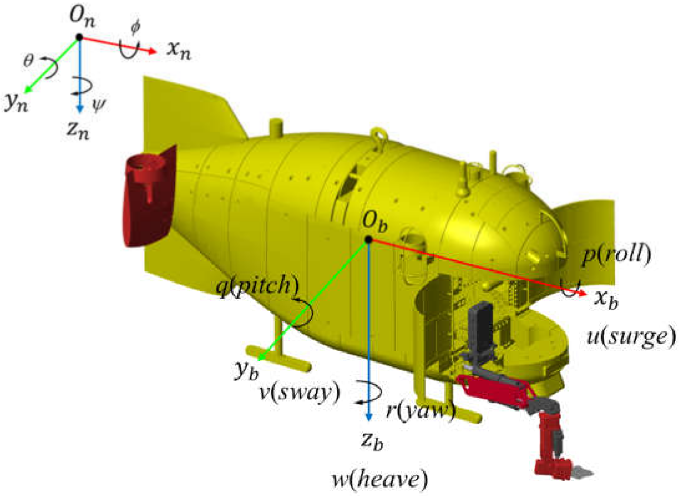
2.1. Vehicle Dynamics

The ARV dynamic model involves two reference frames, as shown in Figure 1. One is the inertial-fixed frame {n}, another is the body-fixed frame {b} fixed at the center of buoyancy (COB) of the ARV. Adopting the SNAME notation [35], the vehicle’s dynamic model considering the manipulator disturbances, hydrodynamic effects, unknown external disturbances can be written in a compact matrix form as [34]:

$$\begin{array}{l}{\rm M}\dot{\nu }+C(\nu )\nu +D(\nu )\nu +g(\eta )={\tau }_v+{\mathsf{\tau }}_m+{\mathsf{\tau }}_u\\ \dot{\eta }=J(\eta )\nu \end{array}$$

(1)

where $\eta ={[x y z\varphi \theta \psi ]}^T$ denotes the position and attitude vector in the inertial-fixed frame and $\nu ={[u v w p q r]}^T$ is the linear and angular velocities expressed in the body-fixed frame. $J(\eta )\in {ℝ}^{6\times 6}$ is the Euler angle mapping matrix from the inertial-fixed frame to the body-fixed frame. ${\rm M}\in {ℝ}^{6\times 6}$ is the inertia matrix, including the effects of added mass, $C(v)\in {ℝ}^{6\times 6}$ is the Coriolis and centripetal matrix, $D(v)\in {ℝ}^{6\times 6}$ represents the hydrodynamic damping matrix, $g(\eta )\in {ℝ}^6$ is the vector of gravitational/buoyancy forces and moments expressed in the body-fixed frame. Finally, ${\tau }_m\in {ℝ}^6$ defines the vector of coupling reaction forces between the manipulator and the vehicle. ${\tau }_u\in {ℝ}^6$ represents the vector of unknown external disturbances. ${\tau }_v\in {ℝ}^6$ is the resultant vector of force/moment generated by thrusters. The vector of the thruster forces $u_T\in {ℝ}^6$ produced by each thruster can be calculated by:

$$u_T=B^{-1}{\tau }_v$$

(2)

where $B\in {ℝ}^{6\times 6}$ is a nonsingular thruster distribution matrix. Refer to Appendix B for further details about the thruster arrangement.

To simplify the vehicle dynamics model and reduce the computational burden, proper simplification should be made. As the Haidou-1 ARV usually works in the deep-sea circumstance, the effect of wave effect and the ocean current is not considered here. The interaction force between the optical fiber and the vehicle is negligible since it is very small and hard to model accurately. The hydrodynamic coefficients of Haidou-1 ARV are obtained by the computational fluid dynamics (CFD) method. Refer to Appendix A for further details about the vehicle dynamics model.

As the controller is normally designed in task space, it is necessary to establish the vehicle dynamics in the inertial-fixed frame. Using the following kinematic transformation equations (assuming that $J(\eta )$ is nonsingular):

$$\begin{array}{l}{M}_{\eta }(\eta )=J^{-T}(\eta )M{J}^{-1}(\eta )\\ C_{\eta }(v,\eta )=J^{-T}(\eta )\left[C(v)-M{J}^{-1}(\eta )\dot{J}(\eta )\right]J^{-1}(\eta )\\ D_{\eta }(v,\eta )=J^{-T}(\eta )D(v)J^{-1}(\eta )\\ {\tau }_{m\eta }=J^{-T}(\eta ){\tau }_m\\ {\tau }_{u\eta }=J^{-T}(\eta ){\tau }_u\\ g_{\eta }(\eta )=J^{-T}(\eta )g(\eta )\\ {\tau }_{\eta }=J^{-T}(\eta ){\tau }_{\nu }\end{array}$$

(3)

The vehicle dynamics (1) can be rewritten in the inertial-fixed frame as:

$$M_{\eta }(\eta )\ddot{\eta }+C_{\eta }(v,\eta )\dot{\eta }+D_{\eta }(v,\eta )\dot{\eta }+g_{\eta }(\eta )={\tau }_{\eta }+{\tau }_{m\eta }+{\tau }_{u\eta }$$

(4)

By introducing a constant diagonal matrix $\widehat{M}$, the vehicle dynamics (4) can be rewritten as:

$$\ddot{\eta }={\widehat{M}}^{-1}\left({\tau }_{\eta }+f(\eta ,v)\right)$$

(5)

where $f(\eta ,v)$ represents the total disturbance, including the internal nonlinear dynamics and external disturbance, and it is defined as follows:

$$f(\eta ,v)={\tau }_{m\eta }+{\tau }_{u\eta }-C_{\eta }(v,\eta )\dot{\eta }-D_{\eta }(v,\eta )\dot{\eta }-g_{\eta }(\eta )+(\widehat{M}-M_{\eta }(\eta ))\ddot{\eta }$$

(6)

To facilitate controller design, the following assumptions are required.

Assumption 1.

The time derivative of total disturbance$f(\eta ,v)$exists and is bounded.

Assumption 2.

The pitch angle is restricted to$\left|\theta \right|<\pi /2$.

Since the ARV is a mechanical system, $f(\eta ,\nu )$ will not change infinitely fast. Therefore, assuming that $\dot{f}(\eta ,\nu )$ is bounded is a valid assumption. According to Assumption 2, the inverse of the Jacobian matrix $J(\eta )$ exists. For the station-keeping operations, the desired pitch angle is 0 rad. The fully actuated vehicle has the ability to keep the pitch angle sufficiently far from $\pm \pi /2$ radian; besides, the vehicle has metacentric restoring forces. Thus, the pitch angle is unlikely to violate this restriction [36]. Assumption 2 is reasonable.

2.2. Manipulator Dynamics

In this paper, the Newton-Euler method was used to derive the dynamic model of the deep-sea manipulator. This method starts with a forward recursion algorithm that calculates the velocity and acceleration information of each link starting from the base and moving towards the end-effector [37]:

$$\begin{array}{c}{\omega }_{i+1}^{i+1}=R_i^{i+1}{\omega }_i^i+{\dot{q}}_{i+1}{\widehat{Z}}_{i+1}\hfill \\ {\dot{\omega }}_{i+1}^{i+1}=R_i^{i+1}{\dot{\omega }}_i^i+R_i^{i+1}\left({}^i\omega {}_i\times {\dot{q}}_{i+1}{{}^{i+1}\widehat{Z}}_{i+1}\right)+{\ddot{q}}_{i+1}{\widehat{Z}}_{i+1}\hfill \\ v_{i+1}^{i+1}=R_i^{i+1}\left(v_i^i+{\omega }_i^i\times P_{i+1}^i\right)\hfill \\ {\dot{v}}_{i+1}^{i+1}=R_i^{i+1}\left({\dot{v}}_i^i+{}^i\dot{\omega }{}_i\times P_{i+1}^i+{\omega }_i^i\times \left({\omega }_i^i\times P_{i+1}^i\right)\right)\hfill \\ {\dot{v}}_{c,i+1}^{i+1}={\dot{v}}_{i+1}^{i+1}+{\dot{\omega }}_{i+1}^{i+1}\times P_{c,i+1}^{i+1}+{\omega }_{i+1}^{i+1}\times ({\omega }_{i+1}^{i+1}\times P_{c,i+1}^{i+1})\hfill \end{array}$$

(7)

where $q_{i+1}$ and ${\dot{q}}_{i+1}$ are the joint position and velocity of joint i, $z_{i+1}={[0 0 1]}^T$, ${}^{i+1}R{}_i$ is the rotation matrix from frame {i} to frame {i + 1}, ${}^i\omega {}_i$ and ${}^i\dot{\omega }{}_i$ are the angular velocity and angular acceleration of link i w.r.t. frame {i}. ${}^{i}v{}_i$ and ${}^i\dot{v}{}_i$ are the linear velocity and linear acceleration of link i w.r.t. frame {i}. ${{}^{i+1}\dot{v}}_{c,i+1}$ represents the linear acceleration of the center of mass (COM) of link i + 1 expressed in frame {i + 1}. ${{}^{i}P}_{i+1}$ is the position vector from joint i to joint i + 1 expressed in frame {i}. ${{}^{i+1}P}_{c,i+1}$ is the position vector from joint i + 1 to the COM of link i + 1 expressed in frame {i + 1}.

Then backward recursion algorithm performs the force and moment balance on each link and iterates backward from the end effector to the manipulator base. The generalized force and moment of link i can be determined by:

$$\begin{array}{l}{}^{i}F{}_i=M_i{\dot{v}}_{c,i}\\ {}^{i}N{}_i=I_i{}^i\dot{\omega }{}_i+{}^i\omega {}_i\times (I_i{}^i\omega {}_i)\end{array}$$

(8)

where $M_i$ and $I_i$ are the mass matrix and the inertia matrix of link i, respectively.

In the deep ocean environment, each link of the underwater manipulator will be affected by its self-motion and uniform flow. Due to unpredictable and weak ocean currents in the deep sea, only self-motion is taken into account here. The hydrodynamic forces exerted on the manipulator are similar to the vehicle, consisting of additional mass force, buoyancy, drag force, etc. As the manipulator moves slowly, the additional mass force acting on the link can be neglected.

The drag force acting on the link i is calculated as [38]:

$$\begin{array}{l}{f}_{hi}=\frac{1}{2}\rho C_{d}D{\displaystyle {\int }_0^{l_i}‖v(x)‖v(x)dx}\\ n_{hi}=\frac{1}{2}\rho C_{d}D{\displaystyle {\int }_0^{l_i}‖v^n(x)‖\left\{{[x,0,0]}^T\times v^n(x)\right\}dx}\end{array}$$

(9)

where

$$\begin{array}{l}v(x)={}^{i}v{}_i+{}^i\omega {}_i\times [x,0,0]={[v_1(x),v_2(x),v_3(x)]}^T\\ v^n(x)={[0,v_2(x),v_3(x)]}^T\end{array}$$

where ρ is the density of seawater, C_d is the drag coefficient, C_m is the inertia force coefficient, A is the projected area that is perpendicular to the velocity of the incoming flow, D is the cross-sectional area of the object, l_i is the length of link i, the empirical values of C_d = 1.0 is used here [39].

The vectors of the interaction of forces and moments between two adjacent links are calculated as follows:

$$\begin{array}{l}{}^{i}f{}_i={}^{i}R{}_{i+1}{}^{i+1}f{}_{i+1}+{}^{i}F{}_i+m_i{g}_i+b_i+f_{hi}\\ {}^{i}n{}_i={}^{i}R{}_{i+1}{}^{i+1}n{}_{i+1}+{}^{i}N{}_i+{}^{i}P{}_{i+1}\times ({}^{i}R{}_{i+1}{}^{i+1}f{}_{i+1})+P_{ci}^i\times {}^{i}F{}_i-P_{ci}^i\times m_{i}g-P_{bi}^i\times b_i+n_{hi}\end{array}$$

(10)

where $P_{bi}^i$ is the position vector from the COB of link i to the origin of frame {i}. $m_i$ is the mass of the link i, $b_i$ is the vector of buoyancy of link i.

The dynamic coupling force/moment acting on the vehicle can be calculated as follows:

$${\tau }_m=\left[\begin{array}{c}{}^{b}R{}_0{}^{0}f{}_0\\ {}^{b}R{}_0{}^{0}n{}_0+{}^{b}P{}_0\times ({}^{b}R{}_0{}^{0}f{}_0)\end{array}\right]$$

(11)

where $f_0^0$ and $t_0^0$ are the vectors of the force and the moment exerted on the manipulator base. $P_0^b$ is the position vector from the body-fixed frame {b} to the manipulator base frame {0}.

Due to the particular operating environment and irregular geometric shape, the dynamics of the deep-sea manipulator are more complicated than on-shore industrial manipulators. The hydrodynamic coefficients are difficult to measure or estimate accurately, and the joint friction term is also hard to model accurately owing to the outside seawater pressure. Furthermore, the manipulator dynamics involve the iterative algorithm, which is computationally expensive. Thus, the control scheme should not rely on the dynamic model of the deep-sea manipulator.

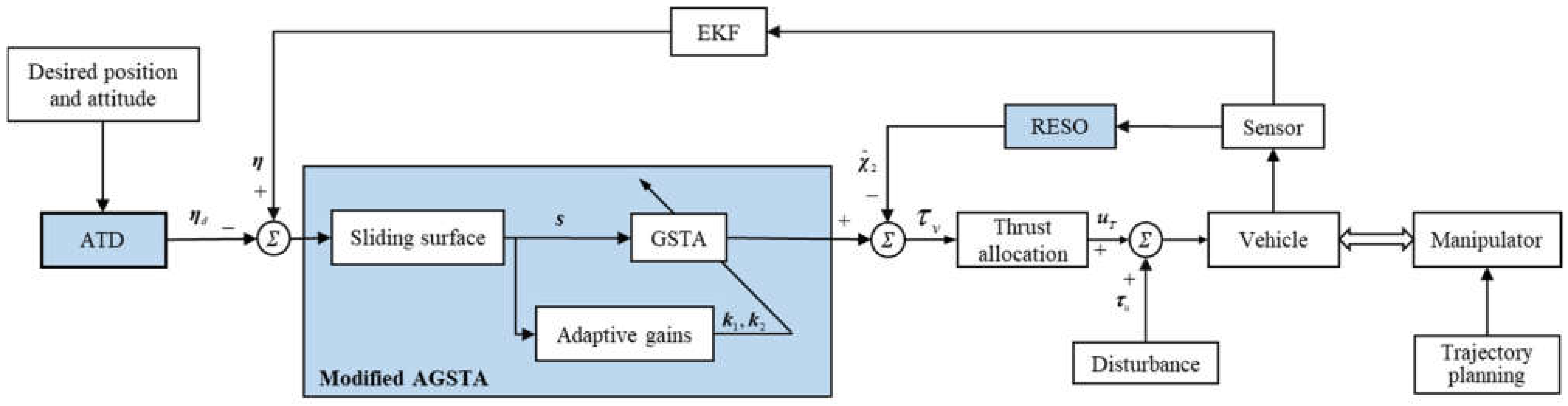
3. Controller Design

In this section, the design of the proposed control scheme for the station-keeping control of ARVs is addressed. The control objective is to stabilize the vehicle in a desired position and attitude while the manipulator performs the manipulation task. Inspired by the methodology presented in [34], we proposed a new adaptive law for the GSTA. The ATD and RESO are used to enhance the control performance of modified AGSTA. Figure 2 presents the control block diagram.

3.1. Adaptive Tracking Differentiator

In the free-floating manipulation, the vehicle has difficulty tracking the fast change reference signal due to larger inertia. Besides, the differential signal is usually extracted by the backward difference method, which is very sensitive to noise. To overcome these problems, Cai, Mingxue, et al. [16] proposed the ATD, which can provide the reference signal and its derivative with a smooth and adjustable process. Compared to the conventional tracking differentiator, ATD enhances the ability to adapt different step signals with the variable filter coefficient and fast coefficient.

The discrete form of the ATD can be designed as follows:

$$\left\{\begin{array}{l}{r}_0=A/4T^2\hfill \\ h_0=\left\{\begin{array}{ll}4h\hfill & without noise\hfill \\ (A/A_n+1)h\hfill & with noise\hfill \end{array}\right.\hfill \\ y_1(k+1)=y_1(k)+h{y}_2(k)\hfill \\ y_2(k+1)=y_2(k)+hfhan(y_1(k)-x(k),y_2(k),r_0,h_0)\hfill \end{array}\right.$$

(12)

where T is the desired transient time of the reference signal, A is the amplitude of step signal, h is the sampling period, r₀ is the fast coefficient, h₀ is the filter coefficient, $A_n$ denotes the amplitude of the noise signal, $x(k)$ is the input signal of ATD, $y_1(k)$ and $y_2(k)$ represent the target reference signal and corresponding derivative, respectively. $fhan(\cdot )$ is denoted as the optimal synthetic rapid control function which is proposed as:

$$\left\{\begin{array}{l}{a}_0=r_0{h}_0^2\hfill \\ a_1=h_0{x}_2\hfill \\ a_2=x_1+a_1\hfill \\ a_3=\sqrt{a_0(a_0+8\left|a_2\right|)}\hfill \\ b_0=a_1+sign(a_2)(a_3-a_0)/2\hfill \\ b_1=[sign(a_2+a_0)-sign(a_2-a_0)]/2\hfill \\ b_2=(a_1+a_2-b_0)b_1+b_0\hfill \\ b_3=[sign(b_2+a_0)-sign(b_2-a_0)]/2\hfill \\ fhan(x_1,x_2,r_0,h_0)=-r_0[b_2/a_0-sign(b_2)]b_3-r_{0}sign(b_2)\hfill \end{array}\right.$$

(13)

3.2. Reduced-Order Extended State Observer

In this section, an extended state observer (ESO) is developed to estimate the total disturbance term in real-time. Considering that the system state variables of ARV can be measured relatively accurately, there is no need to estimate it. Besides, the initial estimation error will cause an initial peaking phenomenon. Therefore, a reduced-order ESO is preferred.

To use RESO, we introduce a change of variables. Define ${\chi }_1=\dot{\eta }$, ${\chi }_2={\widehat{M}}^{-1}f(\eta ,v)$.

Note that Assumption 1 indicates that the time derivative of the total disturbance term $f(\eta ,v)$ exists. Therefore, the vehicle dynamics (5) can be extended as the following state-space form:

$$\left\{\begin{array}{l}{\dot{\chi }}_1={\widehat{\chi }}_2+{\widehat{M}}^{-1}{\tau }_{\eta }\hfill \\ {\dot{\chi }}_2={\widehat{M}}^{-1}\dot{f}(\eta ,v)\hfill \end{array}\right.$$

(14)

Defined ${\widehat{\chi }}_1$ and ${\widehat{\chi }}_2$ as the estimated value of the state variables. The corresponding estimation error is defined as ${\tilde{\chi }}_i={\chi }_i-{\widehat{\chi }}_i$, i = 1, 2. Then the RESO is designed as [40]:

$$\left\{\begin{array}{l}{\dot{\widehat{\chi }}}_1={\widehat{\chi }}_2+{\widehat{M}}^{-1}{\tau }_{\eta }+{\beta }_1{\tilde{\chi }}_1\hfill \\ {\dot{\widehat{\chi }}}_2={\beta }_2{\tilde{\chi }}_1\hfill \end{array}\right.$$

(15)

where ${\beta }_i\in {ℝ}^{6\times 6}, i=1, 2,$ are the corresponding observer gains. Using the bandwidth-parameterization method proposed in [41], all observer poles can be placed at $-{\omega }_i$. To this end, the observer gains can be selected as follows:

$$\left\{\begin{array}{l}{\beta }_1=diag(2{\omega }_1,2{\omega }_2,2{\omega }_3,2{\omega }_4,2{\omega }_5,2{\omega }_6)\hfill \\ {\beta }_2=diag({\omega }_1,{\omega }_2,{\omega }_3,{\omega }_4,{\omega }_5,{\omega }_6)\hfill \end{array}\right.$$

(16)

As a result, the RESO has only one parameter to be tuned in one DOF, which is the observer bandwidth. It should be noted that a smaller estimation error can be obtained by increasing the bandwidth of RESO. However, the RESO will become more sensitive to the measurement noise. Therefore, the observer bandwidth should be selected to achieve a trade-off between the observer performance and the capability of noise tolerance.

3.3. Modified AGSTA Design

There exist two phases for the SMC, i.e., the sliding phase and reaching phase. For the sliding phase, a linear sliding surface is chosen as follows:

$$s=\dot{e}+ce$$

(17)

where $s={[s_1, s_2, \dots s_6]}^T$, $e=\eta -{\eta }_d$ is the error vector. $c=diag(c_1,c_2\cdots c_6)$ is a diagonal positive definite matrix, which determines the convergence rate of the error.

To obtain good control performance during the reaching phase and alleviate chattering, the following GSTA will be used:

$$\begin{array}{l}{\dot{s}}_i=-k_{1i}{\varphi }_{1i}(s_i)+{\varpi }_i\\ {\dot{\varpi }}_i=-k_{2i}{\varphi }_{2i}(s_i)\end{array}$$

(18)

where

$$\begin{array}{l}{\varphi }_{1i}(s_i)={\mu }_{1i}{\left|s_i\right|}^{\frac{1}{2}}sgn(s_i)+{\mu }_{2i}{s}_i\\ {\varphi }_{2i}(s_i)=\frac{1}{2}{\mu }_{1i}^{2}sgn(s_i)+\frac{3}{2}{\mu }_{1i}{\mu }_{2i}{\left|s_i\right|}^{\frac{1}{2}}sgn(s_i)+{\mu }_{2i}^2{s}_i\end{array}$$

One can see that for the choice ${\mu }_{2i}=0$, the structure of the standard STA is recovered. The linear growth term ${\mu }_{2i}{s}_i$ in ${\varphi }_{1i}(s_i)$ helps to counteract the effects of state-dependent perturbations, which can exponentially increase in time.

The adaptive gains $k_{1i}(t)$ and $k_{2i}(t)$ are updated as:

$$\begin{array}{l}{\dot{k}}_{1i}(t)=\left\{\begin{array}{l}{{\displaystyle \ell }}_i\left|s_i\right|>{\sigma }_i\hfill \\ -r_i{k}_{1i}>k_{1i\min },\left|s_i\right|\le {\sigma }_i\hfill \\ 0k_{1i}\le k_{1i\min },\left|s_i\right|\le {\sigma }_i\hfill \end{array}\right.\\ k_{2i}(t)=2{\epsilon }_i{k}_{1i}+{\beta }_i+4{\epsilon }_i^2\end{array}$$

(19)

where ${\mu }_{1i}, {\mu }_{2i}, {\omega }_i, r_i, {\sigma }_i, {\beta }_i, k_{1i\min }, {\sigma }_i$ and ${\epsilon }_i$ are arbitrary positive constants. $r_i$ is utilized to adjust the decrease rate of $k_{1i}$, which avoids overestimating the control gains. Note that $r_i$ is set to ${\mathcal{l}}_i$ in many papers [42,43,44], which may not be the best choice. ${\sigma }_i$ denotes the predefined neighborhood of zero, smaller ${\sigma }_i$ can ensure lower steady-state error but increase the chattering effect as well. $k_{1i\min }$ is used to maintain the control performance when the sliding variable converges to the region $\left|s_i\right|<{\sigma }_i$. When $k_{1i}\le k_{1i\min }$ and $\left|s_i\right|\le {\sigma }_i$, ${\dot{k}}_{1i}(t)$ is set to 0 instead of ${\ell }_i$, which avoids the control gains are varying in a zigzag motion.

Finally, combining the RESO and modified AGSTA, the control scheme for the station-keeping control of ARV is given as follows:

$${\tau }_{\nu }=J^T\widehat{M}[{\widehat{\ddot{\eta }}}_d+c\dot{e}-{\widehat{\chi }}_2+\upsilon ]$$

(20)

where ${\widehat{\ddot{\eta }}}_d$ denotes the nominal value of the second derivative of the reference signal, $\upsilon ={[{\upsilon }_1,{\upsilon }_2,\cdots ,{\upsilon }_6]}^T$, and each element of this vector is given as:

$${\upsilon }_i=-k_{1i}{\varphi }_{1i}(s_i)-{\displaystyle \int k_{2i}{\varphi }_{2i}(s_i)}$$

(21)

It should be noted that we cannot obtain ${\ddot{\eta }}_d$ with the ATD. Nevertheless, we can replace it with a nominal value, such as 0. The corresponding error will be treated as an unknown disturbance.

3.4. Stability Analysis

The following lemma is used for the stability analysis.

Lemma 1.

[45]. Consider a nonlinear system $\dot{x}=f(t,x)$. Suppose there exists a continuous positive definite function $V(x)$, which satisfies $\dot{V}(x)\le -\lambda V^{\alpha }(x)$. Then, the system state arrives at the equilibrium point in a finite-time $t_s$ which satisfies $t_s\le V^{(1-\alpha )}(0)/\lambda (1-\alpha )$.

Substituting the controller (20) into the vehicle dynamics (5) yields the closed-loop dynamics, then take the i-th DOF to analyze for convenience; we have

$$\begin{array}{l}\dot{s}=-k_1[{\mu }_1{\left|s\right|}^{\frac{1}{2}}sgn(s)+{\mu }_{2}s]+\varpi \\ \dot{\varpi }=-k_2[\frac{1}{2}{\mu }_1^{2}sgn(s)+\frac{3}{2}{\mu }_1{\mu }_2{\left|s\right|}^{\frac{1}{2}}sgn(s)]+\dot{h}(t)\end{array}$$

(22)

where $h_i(t)={[{\tilde{\chi }}_2+{\ddot{\eta }}_d-{\widehat{\ddot{\eta }}}_d]}_i$ stands for the estimation error of RESO and ${\ddot{\eta }}_d$ which has been proved to be bounded in [40].

Without loss of generality, Equation (22) can be rewritten in a compact form:

$$\begin{array}{l}\dot{s}=-k_1{\varphi }_1(s)+\varpi \\ \dot{\varpi }=-k_2{\varphi }_2(s)+\dot{h}\end{array}$$

(23)

where

$$\begin{array}{l}{\varphi }_1(s)={\mu }_1{\left|s\right|}^{\frac{1}{2}}sgn(s)+{\mu }_{2}s\\ {\varphi }_2(s)=\frac{1}{2}{\mu }_1^{2}sgn(s)+\frac{3}{2}{\mu }_1{\mu }_2{\left|s\right|}^{\frac{1}{2}}sgn(s)\end{array}$$

For the convenience of Lyapunov analysis, a new state vector is introduced here:

$$z={[z_1 z_2]}^T={[{\varphi }_1 (s) \varpi ]}^T$$

(24)

Noting that ${\varphi }_2(s)={\varphi }_1^{\prime }(s){\varphi }_1(s)$ and ${\varphi }_1^{\prime }(s)={\mu }_1/2|s{|}^{\frac{1}{2}}+{\mu }_2$. Then, the time derivative of z is obtained as:

$$\begin{array}{l}{\dot{z}}_1={\varphi }_1^{\prime }(s)[-k_1{z}_1+z_2]\\ {\dot{z}}_2=-{\varphi }_1^{\prime }(s)k_2{z}_1+\dot{h}\end{array}$$

(25)

where $\dot{h}$ is bounded as $\left|\dot{h}\right|\le h_b$. Thus, there exists an unknown bounded function $L(t)$ satisfying $\dot{h}=L(t){\varphi }_1^{\prime }(s)$.

Remark 1.

Note that the differential equations in (25) have discontinuous right-hand sides; the solutions of this differential inclusion are understood in Filippov’s sense [46].

Equation (25) can be rewritten in a vector-matrix format:

$$\dot{z}={\varphi }_1^{\prime }(s)Az$$

(26)

where

$$A=\left[\begin{array}{cc}-k_1& 1\\ -k_2+L(t)& 0\end{array}\right]$$

Then, the following Lyapunov candidate function will be used to prove the closed-loop stability.

$$V(z_1,z_2,k_1,k_2)=V_0(z)+\frac{1}{2{\varsigma }_1}{(k_1-k_1^{*})}^2+\frac{1}{2{\varsigma }_2}{(k_2-k_2^{*})}^2$$

(27)

where ${\varsigma }_1$, ${\varsigma }_2$, $k_1^{*}$ and $k_2^{*}$ are positive constants and $V_0(z)$ is given by:

$$V_0(z)=(\beta +4{\epsilon }^2)z_1^2-4\epsilon z_1{z}_2+z_2^2=z^{T}Pz$$

(28)

$$P=P^T=\left[\begin{array}{cc}\beta +4{\epsilon }^2& -2\epsilon \\ -2\epsilon & 1\end{array}\right]>0$$

Furthermore, it is easy to verify that V(·) is positive definite and radially unbounded. It is noteworthy that P is a positive definite matrix if $\beta$ is an arbitrary positive constant. By using the standard inequality for quadratic forms, we obtain:

$${\lambda }_{\min }\left\{P\right\}\left|\right|z|{|}_2^2\le V_0(z)\le {\lambda }_{\max }\{P\left\}\right|\left|z\right|{|}_2^2$$

(29)

where $\left|\right|z|{|}_2^2={\mu }_1^2|s|+2{\mu }_1{\mu }_2|s{|}^{\frac{3}{2}}+{\mu }_2^2{s}^2+{\varpi }^2$ represents the Euclidean norm. ${\lambda }_{\min }\{\cdot \}$ and ${\lambda }_{\max }\{\cdot \}$ are the minimum and maximum eigenvalues of matrices, respectively. Further, we can derive the following inequality:

$$|s{|}^{\frac{1}{2}}\le \frac{1}{{\mu }_1}||z|{|}_2\le \frac{V_0^{\frac{1}{2}}(z)}{{\mu }_1{\lambda }_{\min }^{\frac{1}{2}}\left\{P\right\}}$$

(30)

The time derivative of $V_0(z)$ is further given as:

$${\dot{V}}_0(z)={\dot{z}}^{T}Pz+z^{T}P\dot{z}={\varphi }_1^{\prime }(s)z^T[A^{T}P+PA]z=-{\varphi }_1^{\prime }(s)z^{T}Qz$$

(31)

where

$$Q=\left[\begin{array}{cc}2k_1(\beta +4{\epsilon }^2)-4\epsilon (k_2-L(t))& k_2-\beta -4{\epsilon }^2-2\epsilon k_1-L(t)\\ k_2-\beta -4{\epsilon }^2-2\epsilon k_1-L(t)& 4\epsilon \end{array}\right]$$

Selecting the gain $k_2=\beta +2\epsilon k_1+4{\epsilon }^2$, the matrix Q will be a positive definite matrix with minimum eigenvalue $2\epsilon$ if $k_1$ satisfies the following inequality:

$$k_1>\frac{L^2(t)}{4\epsilon \beta }+\frac{2\epsilon (\beta +4{\epsilon }^2-L)+\epsilon }{\beta }$$

(32)

Then, the time derivative of $V_0(z)$ satisfies the following inequalities

$${\dot{V}}_0(z)=-{\varphi }_1^{\prime }(s)z^{T}Qz\le -2\epsilon ({\mu }_1/2|s{|}^{\frac{1}{2}}+{\mu }_2)|\left|z\right|{|}_2^2$$

(33)

Substituting (29) and (30) into (33), we can obtain:

$${\dot{V}}_0(z_i)\le -\frac{{\mu }_1^2\epsilon }{{\lambda }_{\min }^{\frac{1}{2}}\{P\}}{V}_0^{\frac{1}{2}}(z)-2{\mu }_2\epsilon \frac{V_0(z)}{{\lambda }_{\max }\left\{P\right\}}\le -\wp V_0^{\frac{1}{2}}(z)$$

(34)

where

$$\wp =\frac{{\mu }_1^2\epsilon }{{\lambda }_{\min }^{\frac{1}{2}}\{P\}}$$

Differentiating the Lyapunov function candidate (27) w.r.t. time yields:

$$\begin{array}{cc}\dot{V}(\cdot )\hfill & ={\dot{V}}_0\left(z\right)+\frac{1}{{\varsigma }_1}\left(k_1-k_1^{*}\right){\dot{k}}_1+\frac{1}{{\varsigma }_2}\left(k_2-k_2^{*}\right){\dot{k}}_2\hfill \\ & \le -\wp V_0^{\frac{1}{2}}\left(z\right)+\frac{1}{{\varsigma }_1}\left(k_1-k_1^{*}\right){\dot{k}}_1+\frac{1}{{\varsigma }_2}\left(k_2-k_2^{*}\right){\dot{k}}_2\hfill \\ & =-\wp V_0^{\frac{1}{2}}\left(z\right)-\frac{{\omega }_1}{\sqrt{2{\varsigma }_1}}\left|k_1-k_1^{*}\right|-\frac{{\omega }_2}{\sqrt{2{\varsigma }_2}}\left|k_2-k_2^{*}\right|+\frac{1}{{\varsigma }_1}\left(k_1-k_1^{*}\right){\dot{k}}_1\hfill \\ & +\frac{1}{{\varsigma }_2}\left(k_2-k_2^{*}\right){\dot{k}}_2+\frac{{\omega }_1}{\sqrt{2{\varsigma }_1}}\left|k_1-k_1^{*}\right|+\frac{{\omega }_2}{\sqrt{2{\varsigma }_2}}\left|k_2-k_2^{*}\right|\hfill \end{array}$$

(35)

By using the well-known inequality $\sqrt{x^2+y^2+z^2}\le \left|x\right|+\left|y\right|+\left|z\right|$ on (35), the following inequality is obtained

$$-\wp V_0^{\frac{1}{2}}\left(z_i\right)-\frac{{\omega }_1}{\sqrt{2{\varsigma }_1}}\left|k_1-k_1^{*}\right|-\frac{{\omega }_2}{\sqrt{2{\varsigma }_2}}\left|k_2-k_2^{*}\right|\le -\hslash \sqrt{V\left(·\right)}$$

(36)

where

$$\hslash =\min (\wp ,{\omega }_1,{\omega }_2)$$

As indicated in [47], $k_1$ and $k_2$ are bounded. Therefore, there exist positive constants $k_1^{*}$ and $k_2^{*}$ satisfying $k_1-k_1^{*}<0$ and $k_2-k_2^{*}<0$ for $\forall t\ge 0$.

Then, the time derivative of $V(z_1,z_2,k_1,k_2)$ can be rewritten as:

$$\begin{array}{l}\dot{V}(\cdot )\le -\hslash \sqrt{V(\cdot )}-\left|k_1-k_1^{*}\right|\left(\frac{1}{{\varsigma }_1}{\dot{k}}_1-\frac{{\omega }_1}{\sqrt{2{\varsigma }_1}}\right)-\left|k_2-k_2^{*}\right|\left(\frac{1}{{\varsigma }_2}{\dot{k}}_2-\frac{{\omega }_2}{\sqrt{2{\varsigma }_2}}\right)\\ =-\hslash \sqrt{V(\cdot )}+\vartheta \end{array}$$

(37)

where

$$\vartheta =-\left|k_1-k_1^{*}\right|\left(\frac{1}{{\varsigma }_1}{\dot{k}}_1-\frac{{\omega }_1}{\sqrt{2{\varsigma }_1}}\right)-\left|k_2-k_2^{*}\right|\left(\frac{1}{{\varsigma }_2}{\dot{k}}_2-\frac{{\omega }_2}{\sqrt{2{\varsigma }_2}}\right)$$

Finally, some specific conditions should be discussed for accomplishing the proof. For further analysis of $\dot{V}(\cdot )$, its sign should be discussed in three conditions.

When $\left|s\right|>\sigma$, ${\dot{k}}_1=\ell$, and the term $\vartheta$ is computed as:

$$\vartheta =-\left|k_1-k_1^{*}\right|\left(\frac{1}{{\varsigma }_1}\ell -\frac{{\omega }_1}{\sqrt{2{\varsigma }_1}}\right)-\left|k_2-k_2^{*}\right|\left(\frac{1}{{\varsigma }_2}2\epsilon \ell -\frac{{\omega }_2}{\sqrt{2{\varsigma }_2}}\right)$$

(38)

By selecting $\ell ={\omega }_1\sqrt{{\varsigma }_1/2}$ and $\epsilon ={\omega }_2\sqrt{{\varsigma }_2/2}/2\ell$, the term $\vartheta =0$ can be met. Then, Equation (37) can be rewritten as:

$$\dot{V}(·)\le -\hslash \sqrt{V(·)}$$

(39)

The gain $k_1$ will increase monotonically based on adaptive law until the condition (32) is reached. Then the sliding variable will reach the domain $\left|s\right|\le \sigma$ in the finite time according to Lemma 1.

When $k_{1i}>k_{1i\min }$ and $\left|s_i\right|\le {\sigma }_i$, ${\dot{k}}_1=-r$, $\vartheta$ is computed as:

$$\vartheta =\left|k_1-k_1^{*}\right|\left(\frac{1}{{\varsigma }_1}r+\frac{{\omega }_1}{\sqrt{2{\varsigma }_1}}\right)+\left|k_2-k_2^{*}\right|\left(\frac{1}{{\varsigma }_2}2\epsilon r+\frac{{\omega }_2}{\sqrt{2{\varsigma }_2}}\right)$$

(40)

It is obvious that ${\dot{k}}_1<0$ and $\vartheta >0$. Thus the sign of $\dot{V}(\cdot )$ is uncertain, which means $\left|s\right|$ may become greater than $\sigma$ with the decrease of $k_1$. Once the sliding variable exceeds this domain, it will return to the domain $\left|s\right|\le \sigma$ in finite time, as discussed above. It is noted that the condition of $k_1\le k_{1\min }$ and $\left|s\right|\le \sigma$ is similar to that of $k_1>k_{1\min }$ and $\left|s\right|\le \sigma$. Hence we omit the corresponding discussion.

Finally, we can conclude that the sliding variable will converge to the predefined neighborhood of origin in the finite time and remain in a larger domain $\left|s\right|\le \overline{\sigma },\overline{\sigma }>\sigma$ for all subsequent time. Since we use a linear sliding surface, the error vector will confine to the neighborhood of origin asymptotically. The whole system is stable and bounded in finite time.

4. Simulation Results

To validate the feasibility and efficiency of the proposed control scheme, simulations will be conducted on a realistic model Haidou-1 ARV in the MATLAB/Simscape software environment.

4.1. Description of the Simulation System

The ARV model considered in the simulation is composed of a 6 DoFs vehicle and a 6 DoFs deep-sea electric manipulator and is operating in the 11,000 m deep sea. The vehicle has six thrusters in total to provide the station-keeping capabilities, including two vertical thrusters, two side thrusters, and two rotatable thrusters (in the stern side). The thrust force saturation is considered in simulation, and the thrust force can range from −146.9 N to 231.6 N. The vehicle can be fully actuated when the manipulator performs underwater manipulation tasks.

The manipulator mounted on the bow part of the vehicle is a 7-function (with 6 DoFs and 1 clamping function) electric manipulator that can operate in 11,000 m deep sea. The Denavit-Hartenberg (D-H) parameters of the deep-sea electric manipulator are specified in

Table 1. D-H parameters for the deep-sea electric manipulator.

Joint i	$a_{i-1}$ (mm)	$d_i$ (mm)	${\alpha }_{i-1}$ (deg)	Joint Limit (deg)
1	0	0	90	−30~90
2	130.4	138.22	90	−30~90
3	641.8	0	0	−90~30
4	220.2	442.64	90	−90~90
5	21.5	0	−90	0~90
6	−48.1	239.60	90	−180~180

, and the manipulator weighs 36.6 kg in water.

To make the simulation more consistent with the realistic scenario. The sensor measurement noises should be taken into consideration in the simulation. The following sensor noises are added: zero-mean Gaussian noises with the variance of 1 × 10⁻⁴ are added to the ideal vehicle position signals; zero-mean Gaussian noises with the variance of 2.74 × 10⁻⁵ are added to the ideal vehicle attitude signals; zero-mean Gaussian noises with the variance of 2.5 × 10⁻⁷ are added to the ideal vehicle velocity signals. The measurement signals are handled by an extended Kalman filter (EKF) and then used as the controller’s input signals, as shown in Figure 2.

Moreover, the parameters of the dynamic model used in the controller are assumed to be inaccurate and have about 30% parameter uncertainties. In this study, the unknown time-varying external disturbances are simulated using the periodic functions as follows:

$$d_u=\left\{\begin{array}{l}5+3\sin (0.2t+\pi /5)N\hfill \\ 5+4\cos (0.3t+\pi /6)N\hfill \\ 10+8\cos (0.2t)N\hfill \\ 25+16\sin (0.2t)N\cdot m\hfill \\ 30+15\sin (0.2t+\pi /4)N\cdot m\hfill \\ 8+6\cos (0.3t)N\cdot m\hfill \end{array}\right.$$

(41)

Finally, the control scheme is discretized by the explicit Euler method, and the sampling period is set to 0.1 s.

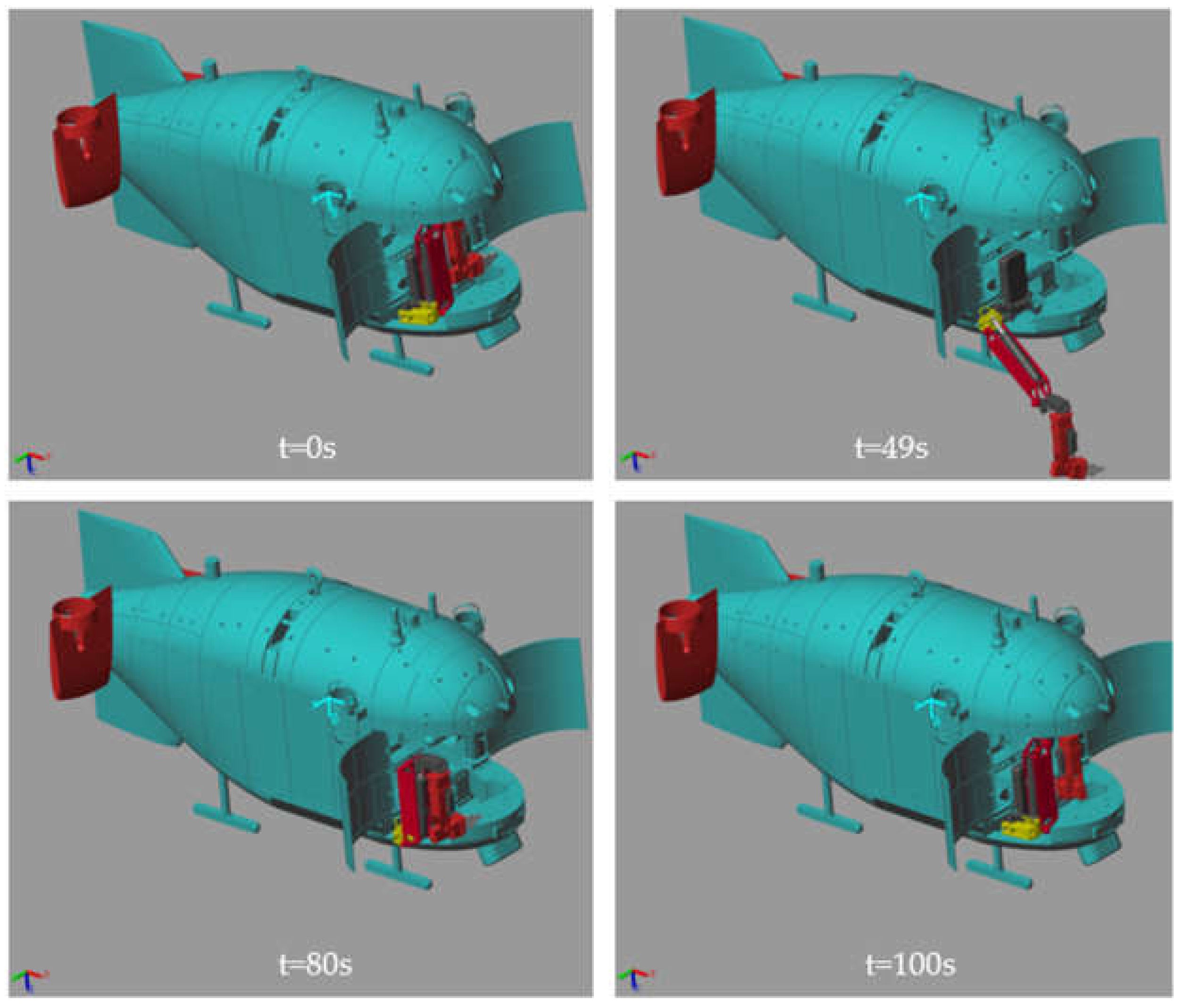
4.2. Description of the Task

In the simulation task, the vehicle performs station-keeping while the manipulator is used to grasp the stationary target. The desired grasping process is illustrated in Figure 3. This simulation is used to verify the station-keeping ability of the ARV after using the proposed controller. In the simulation, the vehicle’s initial state is set as: ${\eta }_0$ = [0.02,0.02,0.03,π/90,π/90,π/90]^T and ${\nu }_0$ = [0.002,0.001,0.002,0.002,0.002,0.001]^T. The manipulator’s initial state is set to $q_0$ = [90°, 90°, −90°, 0°, 90°, 0°]^T. The desired value ${\eta }_d$ and ${\nu }_d$ are all set to 0. The fifth-order polynomial curves are used to plan joint trajectories in the joint space, and the desired joint trajectories are given in Figure 4. The contact process between the gripper and the object to be manipulated is not considered here. We only linearly added the weight of the grabbed target in water to the manipulator’s end-effector in 0.5 s.

Since our work is based on the previous results of J. Guerrero et al. [34] and can therefore be used as benchmarks of the performance of the proposed controller. To evaluate the control performance quantitatively, two performance indexes are defined as follows:

$$CHAT=\frac{1}{N}{\displaystyle \sum _{k=0}^{N-1}\left|{\tau }_{v,k+1}-{\tau }_{v,k}\right|}$$

(42)

$$RMSE=\sqrt{\frac{1}{N}{\displaystyle \sum _{k=0}^{N-1}{e}_k^2}}$$

(43)

where $t_{k+1}-t_k=h>0$ denotes the sampling period, and we denote $f(t_k)=f_k$ with $k=0,1,2\dots N.$ The first performance index calculates the average variation of the control input signals, which can evaluate the chattering effect quantitatively [48]. The second objective function represents the root mean squared error (RMSE), which can assess the control performance. These two performance indexes allow us to trade off chattering reduction ability and tracking control performance of the controller.

The parameter tuning of the controller is treated as a multi-objective optimization problem, and we use the gamultiobj function in MATLAB to solve it. The chosen control parameters are listed in

Table 2. Controller parameters for the simulation.

AGSTA	$\left[c_i,\hspace{0.33em}{\mu }_{1i},\hspace{0.33em}{\mu }_{2i},\hspace{0.33em}{\ell }_i,\hspace{0.33em}{\epsilon }_i,\hspace{0.33em}{\beta }_i,\hspace{0.33em}{k}_{1i}(0),\hspace{0.33em}{\sigma }_i\right]$
$x$	[2.5500, 0.0021, 0.0690, 0.3192, 3.1620, 1.2692, 0.0049, 0.0020]
$y$	[1.5830, 0.0023, 0.1189, 0.7272, 2.1222, 2.5352, 0.0040, 0.0028]
$z$	[5.1820, 0.0031, 0.1628, 0.3680, 1.8180, 1.2795, 0.0063, 0.0066]
$\varphi$	[5.7932, 0.0032, 0.2474, 1.1557, 2.0171, 0.9480, 0.0066, 0.0155]
$\theta$	[4.0165, 0.0030, 0.0609, 0.5230, 3.9955, 3.2493, 0.0080, 0.0079]
$\psi$	[2.8460, 0.0020, 0.2053, 0.7632, 1.4879, 0.6179, 0.0065, 0.0055]
Proposed	$\left[c_i,\hspace{0.33em}{\mu }_{1i},\hspace{0.33em}{\mu }_{2i},\hspace{0.33em}{\ell }_i,\hspace{0.33em}{r}_i,\hspace{0.17em}{k}_{1i}(0),\hspace{0.33em}{k}_{1\min i},\hspace{0.33em}{\epsilon }_i,\hspace{0.33em}{\beta }_i,\hspace{0.33em}{\sigma }_i,{\omega }_i\right]$
$x$	[2.0576, 0.0023, 0.1315, 1.4140, 0.8028, 0.0045, 0.4425, 1.1732, 2.1554, 0.0017, 1.0792]
$y$	[1.0407, 0.0029, 0.2787, 1.1101, 0.9778, 0.0066, 0.6360, 0.6514, 0.7757, 0.0019, 1.1541]
$z$	[3.1099, 0.0065, 0.2468, 1.4638, 0.2408, 0.0050, 0.5251, 0.6666, 1.5306, 0.0031, 0.5379]
$\varphi$	[8.1867, 0.0068, 0.1687, 0.7613, 0.5755, 0.0658, 0.3288, 1.9506, 2.5442, 0.0077, 1.0778]
$\theta$	[3.1722, 0.0269, 0.1682, 0.6937, 0.6108, 0.0068, 0.1132, 0.2298, 1.4234, 0.0032, 1.1901]
$\psi$	[2.3681, 0.0026, 0.1639, 0.8678, 0.5303, 0.0061, 0.4155, 1.6172, 2.6475, 0.0015, 0.5143]

.

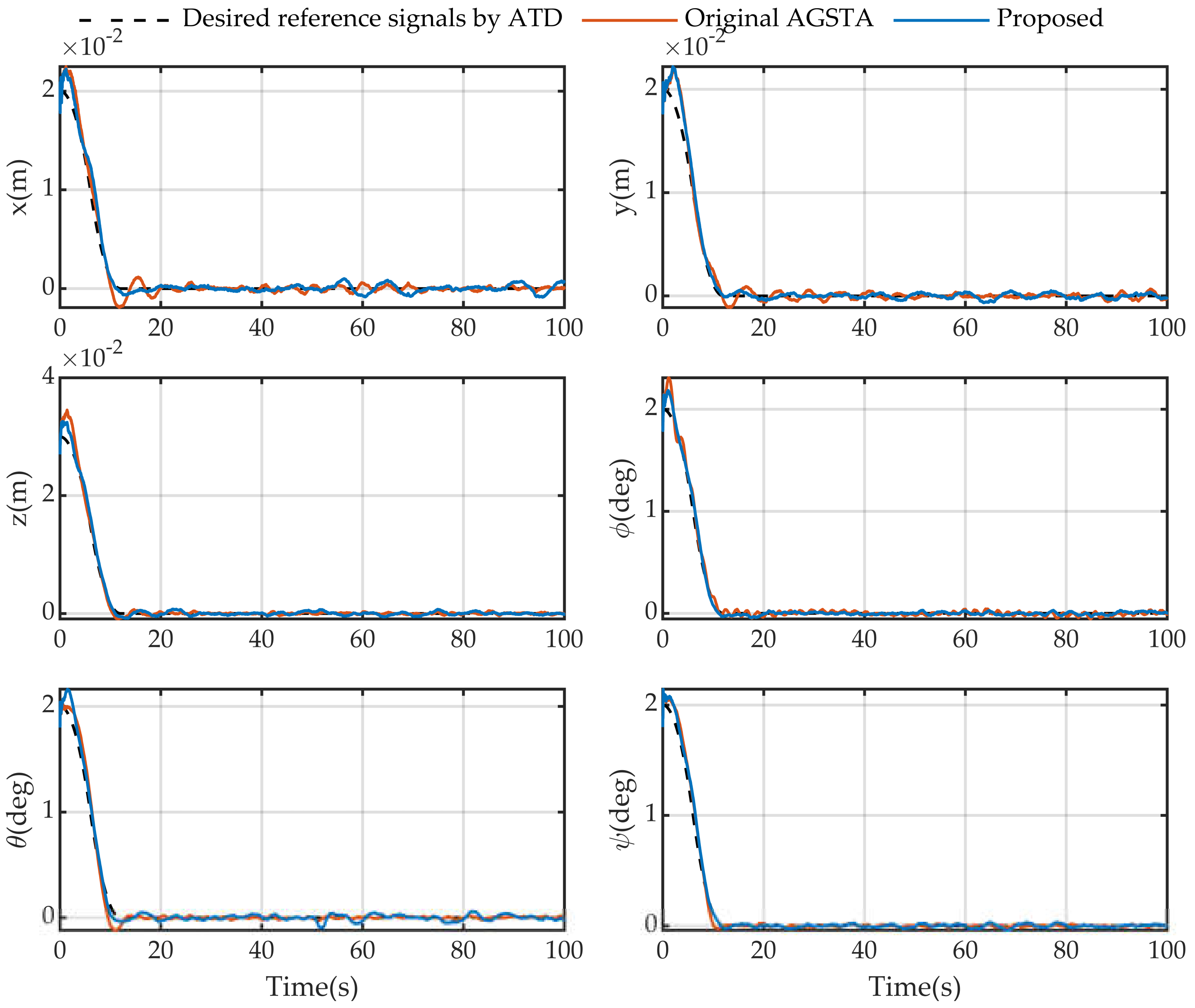
4.3. Results and Discussions

Figure 5 depicts the time responses of vehicle state variables during station-keeping control, and Figure 6 displays the corresponding errors. From Figure 5, one can notice that the desired reference signals generated by the ATD are smooth and are reached for both controllers. However, the origin AGSTA controller has a more significant overshoot and steady-state error than the proposed controller. The RMSE values are given in

Table 3. Comparison of performance indices.

State Variables	CHAT		RMSE
	AGSTA	Proposed	AGSTA	Proposed
$x$	0.0363	0.0285	6.1005 × 10−4	5.9895 × 10−4
$y$	0.0749	0.0462	6.0119 × 10−4	5.8173 × 10−4
$z$	0.1045	0.0672	7.5175 × 10−4	5.1327 × 10−4
$\varphi$	0.0903	0.0538	7.5865 × 10−4	5.3599 × 10−4
$\theta$	0.1173	0.0887	7.7607 × 10−4	7.5049 × 10−4
$\psi$	0.1006	0.0662	5.6136 × 10−4	5.5314 × 10−4

, which indicates that the proposed controller has smaller RMSE values than the origin AGSTA controller.

Figure 7 shows the thrust force for each thruster during the simulation. As expected, the thrust forces of the original AGSTA controller exist serious chattering phenomenon. In contrast with the original AGSTA controller, the proposed controller produces a relatively smooth control input which proves the proposed controller has a better chattering reduction ability. A quantitative performance comparison of the chattering is also given in Table 3. The CHAT value of our proposed controller is 61.8%~78% of the original AGSTA controller.

It should be noted that the control parameters of the original AGSTA controller are also tuned by the multi-objective optimization method. Hence, the CHAT value gap between the two controllers is not very obvious. However, when tunning the control parameters of the original AGSTA controller manually, we find it often leads to severe chattering and even becomes unstable. As a result, the parameter tuning process becomes hard. The proposed controller avoids the problems above, making it safer and easier to tune than the original one.

Figure 8 depicts the time trajectories of the sliding variables during the station-keeping control. It can be observed that the sliding variable enters the predefined neighborhood of origin and try to remain there. The evolution of the adaptive gains k₁(t) is depicted in Figure 9; it can be seen that the control gains of the proposed controller increase or decrease in a bounded region. The control gains tend to maintain at a small value. If the sliding variable exceeds the predefined neighborhood of origin, the adaptive gains will increase until it enters this domain again. Figure 9 shows that small control gains are sufficient to resist the disturbances and ensure an ideal sliding mode most of the time. The proposed controller ensures the sliding variable converges to the neighborhood of origin without overestimating control gains.

For the AGSTA controller, the gains k₁(t) keep increasing until the sliding mode is reached, then the gains remain unchanged, ensuring an ideal sliding mode for a while. As the disturbance increases, the sliding mode may be lost, so the gains k₁(t) keep increasing until the sliding mode is reached again. When the disturbance decreases, the gains still maintain this value. As a result, the AGSTA may overestimate the control gains, which leads to an increase in the chattering amplitude.

It should be noted that some papers [43,49] also allow the control gains to decrease according to specific rules. However, the adaptive law proposed in these papers is limited to the conventional super-twisting algorithm, and control gains will vibrate around the set minimum value. Figure 10 compares control gains’ evolution when using the traditional adaptive law and the proposed adaptive law. The magnified view of Figure 10 confirms that gains of traditional adaptive law vary in zigzag motion after arriving at the minimum value. Our proposed adaptive law avoids this problem which helps further mitigate the chattering. It should be noted that zigzag motion induced by traditional adaptive law will only appear after the controller is discretized and becomes severe with the increase of sampling time.

The total disturbance estimated by RESO is presented in Figure 11. The results show that the total disturbance can be effectively estimated and compensated by the RESO. The initial peaking phenomenon due to the initial state estimation error is eliminated. One can see that the estimated total disturbance has a slight phase lag compared to the simulated value because the bandwidth of RESO is restricted to the measurement noise.

5. Conclusions

This paper is dedicated to solving the station-keeping control problem of ARVs for free-floating manipulation. A modified AGSTA enhanced by ATD and RESO is developed. Comparative simulation results on the Haidou-1 ARV demonstrate that the proposed control scheme is more efficient than the original AGSTA controller. The adaptive gains increase or decrease in a bounded region according to the magnitude of the sliding variable. As a result, the sliding variables are confined to a predefined neighborhood of zero without overestimating control gains, thereby reducing the chattering. Besides, the proposed new variable gain strategy completely avoids the adaptive gains varying in zigzag motion near the set minimum value and is not affected by the sampling time.

In future work, pool experiments will be conducted to demonstrate the effectiveness of our proposed controller. Besides, the proposed controller is designed in the continuous-time domain and discretized by the explicit Euler method, which will introduce discretization chattering [50]. A proper discretization scheme is necessary. Recently, the implicit discretization method has been successfully used to discretize the super-twisting algorithm [51,52], which has been shown theoretically and experimentally to provide significant chattering alleviation. It may apply to our proposed controller and further improve its chattering reduction ability. Besides, the RESO used in this paper is sensitive to noise, which should be handled in future work.

References

1. Fossen, T.I. Guidance and Control of Ocean Vehicles; Wiley: Chichester, UK/New York, NY, USA, 1994; ISBN 978-0-471-94113-2. [Google Scholar]
2. Heshmati-Alamdari, S.; Bechlioulis, C.P.; Karras, G.C.; Nikou, A.; Dimarogonas, D.V.; Kyriakopoulos, K.J. A Robust Interaction Control Approach for Underwater Vehicle Manipulator Systems. Annu. Rev. Control 2018, 46, 315–325. [Google Scholar] [CrossRef]
3. Brignone, L.; Raugel, E.; Opderbecke, J.; Rigaud, V.; Piasco, R.; Ragot, S. First Sea Trials of HROV the New Hybrid Vehicle Developed by IFREMER. In Proceedings of the OCEANS 2015—Genova, Genova, Italy, 18–21 May 2015; IEEE: Genova, Italy, 2015; pp. 1–7. [Google Scholar]
4. Side, Z.; Yuh, J. Experimental Study on Advanced Underwater Robot Control. IEEE Trans. Robot. 2005, 21, 695–703. [Google Scholar] [CrossRef]
5. Mohan, S.; Kim, J. Coordinated Motion Control in Task Space of an Autonomous Underwater Vehicle–Manipulator System. Ocean Eng. 2015, 104, 155–167. [Google Scholar] [CrossRef]
6. Dai, Y.; Yu, S. Design of an Indirect Adaptive Controller for the Trajectory Tracking of UVMS. Ocean Eng. 2018, 151, 234–245. [Google Scholar] [CrossRef]
7. Londhe, P.S.; Santhakumar, M.; Patre, B.M.; Waghmare, L.M. Task Space Control of an Autonomous Underwater Vehicle Manipulator System by Robust Single-Input Fuzzy Logic Control Scheme. IEEE J. Ocean. Eng. 2016, 1–16. [Google Scholar] [CrossRef]
8. Barbalata, C.; Dunnigan, M.; Petillot, Y. Coupled and Decoupled Force/Motion Controllers for an Underwater Vehicle-Manipulator System. J. Mar. Sci. Eng. 2018, 6, 96. [Google Scholar] [CrossRef] [Green Version]
9. Koval, E.V. Automatic Stabilization System of Underwater Manipulation Robot. In “Oceans Engineering for Today’s Technology and Tomorrow’s Preservation” Proceedings of the OCEANS ’94, Brest, France, 13–16 September 1994; IEEE: Piscataway, NJ, USA.
10. Mclain, T.W.; Rock, S.M.; Lee, M.J. Experiments in the Coordinated Control of an Underwater Arm/Vehicle System. Auton. Robots 1996, 3, 213–232. [Google Scholar] [CrossRef]
11. Antonelli, G.; Cataldi, E. Recursive Adaptive Control for an Underwater Vehicle Carrying a Manipulator. In Proceedings of the 22nd Mediterranean Conference on Control and Automation, Palermo, Italy, 16–19 June 2014; pp. 847–852. [Google Scholar]
12. Lynch, B.; Ellery, A. Efficient Control of an AUV-Manipulator System: An Application for the Exploration of Europa. IEEE J. Ocean. Eng. 2014, 39, 552–570. [Google Scholar] [CrossRef]
13. Huang, H.; Tang, Q.; Li, H.; Liang, L.; Li, W.; Pang, Y. Vehicle-Manipulator System Dynamic Modeling and Control for Underwater Autonomous Manipulation. Multibody Syst. Dyn. 2017, 41, 125–147. [Google Scholar] [CrossRef]
14. Huang, H.; Li, J.; Zhang, G.; Tang, Q.; Wan, L. Adaptive Recurrent Neural Network Motion Control for Observation Class Remotely Operated Vehicle Manipulator System with Modeling Uncertainty. Adv. Mech. Eng. 2018, 10, 168781401880409. [Google Scholar] [CrossRef]
15. Dannigan, M.W.; Russell, G.T. Evaluation and Reduction of the Dynamic Coupling between a Manipulator and an Underwater Vehicle. IEEE J. Ocean. Eng. 1998, 23, 260–273. [Google Scholar] [CrossRef]
16. Cai, M.; Wang, S.; Wang, Y.; Wang, R.; Tan, M. Coordinated Control of Underwater Biomimetic Vehicle-Manipulator System for Free Floating Autonomous Manipulation. IEEE Trans. Syst. Man Cybern. Syst. 2019, 1–11. [Google Scholar] [CrossRef]
17. Rojsiraphisal, T.; Mobayen, S.; Asad, J.H.; Vu, M.T.; Chang, A.; Puangmalai, J. Fast Terminal Sliding Control of Underactuated Robotic Systems Based on Disturbance Observer with Experimental Validation. Mathematics 2021, 9, 1935. [Google Scholar] [CrossRef]
18. Thanh, H.L.N.N.; Vu, M.T.; Mung, N.X.; Nguyen, N.P.; Phuong, N.T. Perturbation Observer-Based Robust Control Using a Multiple Sliding Surfaces for Nonlinear Systems with Influences of Matched and Unmatched Uncertainties. Mathematics 2020, 8, 1371. [Google Scholar] [CrossRef]
19. Vu, M.T.; Le, T.-H.; Thanh, H.L.N.N.; Huynh, T.-T.; Van, M.; Hoang, Q.-D.; Do, T.D. Robust Position Control of an Over-Actuated Underwater Vehicle under Model Uncertainties and Ocean Current Effects Using Dynamic Sliding Mode Surface and Optimal Allocation Control. Sensors 2021, 21, 747. [Google Scholar] [CrossRef] [PubMed]
20. Lima, G.S.; Trimpe, S.; Bessa, W.M. Sliding Mode Control with Gaussian Process Regression for Underwater Robots. J. Intell. Robot. Syst. 2020, 99, 487–498. [Google Scholar] [CrossRef]
21. Sun, C.; Gong, G.; Yang, H. Sliding Mode Control with Adaptive Fuzzy Immune Feedback Reaching Law. Int. J. Control Autom. Syst. 2020, 18, 363–373. [Google Scholar] [CrossRef]
22. Wang, G.; Wu, J.; Zeng, B.; Xu, Z.; Ma, X. A Chattering-Free Sliding Mode Control Strategy for Modular High-Temperature Gas-Cooled Reactors. Ann. Nucl. Energy 2019, 133, 688–695. [Google Scholar] [CrossRef]
23. Shi, X.; Cheng, Y. Fuzzy Adaptive Sliding Mode Control for Unmanned Quadrotor. In Proceedings of the 2020 IEEE/ASME International Conference on Advanced Intelligent Mechatronics (AIM), Boston, MA, USA, 6–9 July 2020; IEEE: Boston, MA, USA, 2020; pp. 1654–1658. [Google Scholar]
24. Qiao, L.; Zhang, W. Trajectory Tracking Control of AUVs via Adaptive Fast Nonsingular Integral Terminal Sliding Mode Control. IEEE Trans. Ind. Inform. 2020, 16, 1248–1258. [Google Scholar] [CrossRef]
25. Wu, X.; Jin, P.; Zou, T.; Qi, Z.; Xiao, H.; Lou, P. Backstepping Trajectory Tracking Based on Fuzzy Sliding Mode Control for Differential Mobile Robots. J. Intell Robot Syst. 2019, 96, 109–121. [Google Scholar] [CrossRef]
26. Vahidi-Moghaddam, A. Disturbance-Observer-Based Fuzzy Terminal Sliding Mode Control for MIMO Uncertain Nonlinear Systems. Appl. Math. Model. 2019, 70, 109–127. [Google Scholar] [CrossRef]
27. Levant, A. Homogeneity Approach to High-Order Sliding Mode Design. Automatica 2005, 41, 823–830. [Google Scholar] [CrossRef]
28. Guo, J. A Novel High Order Sliding Mode Control Method. ISA Trans. 2021, 111, 1–7. [Google Scholar] [CrossRef]
29. González-García, J.; Narcizo-Nuci, N.A.; García-Valdovinos, L.G.; Salgado-Jiménez, T.; Gómez-Espinosa, A.; Cuan-Urquizo, E.; Cabello, J.A.E. Model-Free High Order Sliding Mode Control with Finite-Time Tracking for Unmanned Underwater Vehicles. Appl. Sci. 2021, 11, 1836. [Google Scholar] [CrossRef]
30. Shtessel, Y.; Edwards, C.; Fridman, L.; Levant, A. Sliding Mode Control and Observation; Control Engineering; Springer: New York, NY, USA, 2014; ISBN 978-0-8176-4892-3. [Google Scholar]
31. Pérez-Ventura, U.; Fridman, L. When Is It Reasonable to Implement the Discontinuous Sliding-Mode Controllers Instead of the Continuous Ones? Frequency Domain Criteria. Int. J. Robust Nonlinear Control 2019, 29, 810–828. [Google Scholar] [CrossRef]
32. Moreno, J.A. A Linear Framework for the Robust Stability Analysis of a Generalized Super-Twisting Algorithm. In Proceedings of the International Conference on Electrical Engineering, Toluca, Mexico, 10–13 January 2009. [Google Scholar]
33. Castillo, I.; Fridman, L.; Moreno, J.A. Super-Twisting Algorithm in Presence of Time and State Dependent Perturbations. Int. J. Control 2018, 91, 2535–2548. [Google Scholar] [CrossRef]
34. Guerrero, J.; Torres, J.; Creuze, V.; Chemori, A. Trajectory Tracking for Autonomous Underwater Vehicle: An Adaptive Approach. Ocean Eng. 2019, 172, 511–522. [Google Scholar] [CrossRef] [Green Version]
35. SNAME, T. Nomenclature for Treating the Motion of a Submerged Body through a Fluid. Soc. Nav. Archit. Mar. Eng. Tech. Res. Bull. 1950, 1–5. [Google Scholar]
36. Fischer, N.; Hughes, D.; Walters, P.; Schwartz, E.M.; Dixon, W.E. Nonlinear RISE-Based Control of an Autonomous Underwater Vehicle. IEEE Trans. Robot. 2014, 30, 845–852. [Google Scholar] [CrossRef] [Green Version]
37. Spicer, R.L.; Black, J. Simulating the Dynamics and Control of a Free-Flying Small Satellite with a Robotic Manipulator for 3D Printing. In Proceedings of the AIAA Scitech 2020 Forum; American Institute of Aeronautics and Astronautics, Orlando, FL, USA, 6 January 2020. [Google Scholar]
38. McMillan, S.; Orin, D.E.; McGhee, R.B. Efficient Dynamic Simulation of an Underwater Vehicle with a Robotic Manipulator. IEEE Trans. Syst. Man Cybern. 1995, 25, 1194–1206. [Google Scholar] [CrossRef] [Green Version]
39. Yuguang, Z.; Fan, Y. Dynamic Modeling and Adaptive Fuzzy Sliding Mode Control for Multi-Link Underwater Manipulators. Ocean Eng. 2019, 187, 106202. [Google Scholar] [CrossRef]
40. Ren, C.; Ding, Y.; Ma, S. A Structure-Improved Extended State Observer Based Control with Application to an Omnidirectional Mobile Robot. ISA Trans. 2020, 101, 335–345. [Google Scholar] [CrossRef]
41. Long, Y.; Du, Z.; Cong, L.; Wang, W.; Zhang, Z.; Dong, W. Active Disturbance Rejection Control Based Human Gait Tracking for Lower Extremity Rehabilitation Exoskeleton. Isa Trans 2017, 67, 389–397. [Google Scholar] [CrossRef]
42. Zhang, M.; Guan, Y.; Zhao, W. Adaptive Super-Twisting Sliding Mode Control for Stabilization Platform of Laser Seeker Based on Extended State Observer. Optik 2019, 199, 163337. [Google Scholar] [CrossRef]
43. Lee, S.-D.; Hong Phuc, B.D.; Xu, X.; You, S.-S. Roll Suppression of Marine Vessels Using Adaptive Super-Twisting Sliding Mode Control Synthesis. Ocean Eng. 2020, 195, 106724. [Google Scholar] [CrossRef]
44. Rangel, M.A.G.; Manzanilla, A.; Suarez, A.E.Z.; Muñoz, F.; Salazar, S.; Lozano, R. Adaptive Non-Singular Terminal Sliding Mode Control for an Unmanned Underwater Vehicle: Real-Time Experiments. Int. J. Control Autom. Syst. 2020, 18, 615–628. [Google Scholar] [CrossRef]
45. Polyakov, A. Nonlinear Feedback Design for Fixed-Time Stabilization of Linear Control Systems. IEEE Trans. Autom. Control 2012, 57, 5. [Google Scholar] [CrossRef] [Green Version]
46. Filippov, A.F. Differential Equations with Discontinuous Righthand Sides: Control Systems; Springer Science & Business Media: Berlin, Germany, 2013; Volume 18. [Google Scholar]
47. Shtessel, Y.; Taleb, M. A Novel Adaptive-Gain Supertwisting Sliding Mode Controller: Methodology and Application. Automatica 2012, 48, 759–769. [Google Scholar] [CrossRef]
48. Wang, B.; Brogliato, B.; Acary, V.; Boubakir, A.; Plestan, F. Experimental Comparisons between Implicit and Explicit Implementations of Discrete-Time Sliding Mode Controllers: Towards Chattering Suppression in Output and Input Signals. In Proceedings of the 2014 13th International Workshop on Variable Structure Systems (VSS), Nantes, France, 29 June–2 July 2014; IEEE: Nantes, France, 2014; pp. 1–6. [Google Scholar]
49. Wang, Y.; Zhu, K.; Yan, F.; Chen, B. Adaptive Super-Twisting Nonsingular Fast Terminal Sliding Mode Control for Cable-Driven Manipulators Using Time-Delay Estimation. Adv. Eng. Softw. 2019, 128, 113–124. [Google Scholar] [CrossRef]
50. Brogliato, B.; Polyakov, A. Digital Implementation of Sliding-mode Control via the Implicit Method: A Tutorial. Int. J. Robust Nonlinear Control 2020, rnc.5121. [Google Scholar] [CrossRef]
51. Koch, S.; Reichhartinger, M. Discrete-Time Equivalents of the Super-Twisting Algorithm. Automatica 2019, 107, 190–199. [Google Scholar] [CrossRef]
52. Brogliato, B.; Polyakov, A.; Efimov, D. The Implicit Discretization of the Supertwisting Sliding-Mode Control Algorithm. IEEE Trans. Autom. Control 2020, 65, 3707–3713. [Google Scholar] [CrossRef] [Green Version]
Figure 1. The Haidou-1 ARV and its reference frames.
Jmse 09 01305 g001
Figure 2. Diagram of the station-keeping control framework.
Jmse 09 01305 g002
Figure 3. The process of free-floating manipulation during simulation.
Jmse 09 01305 g003
Figure 4. Planned joint trajectories.
Jmse 09 01305 g004
Figure 5. Time response of the vehicle state variables during station-keeping control.
Jmse 09 01305 g005
Figure 6. Vehicle state errors during station-keeping control.
Jmse 09 01305 g006
Figure 7. Thrust force for each thruster during station-keeping control.
Jmse 09 01305 g007
Figure 8. Time trajectories of sliding variables during station-keeping control.
Jmse 09 01305 g008
Figure 9. Evolution of the adaptive gains k1(t) over time.
Jmse 09 01305 g009
Figure 10. Comparison of adaptive gains between the traditional and proposed adaptive law.
Jmse 09 01305 g010
Figure 11. Comparison of estimated total disturbance and simulated total disturbance.
Jmse 09 01305 g011