3D Numerical Study of the Impact of Macro-Roughnesses on a Tidal Turbine, on Its Performance and Hydrodynamic Wake

Abstract

Biofouling is an important factor to consider when calculating the energetic efficiency of tidal farms. Despite the fact that biofouling effects have been widely investigated in the past for naval applications, very few studies concern tidal turbines. This paper proposes a numerical approach to assess the impact of biofouling on tidal turbines, which is efficient for testing many configurations. Two turbulence models are tested (RANS k-ω SST and LES Smagorinsky) for the motionless blade case to validate them. Then we chose to use the Smagorinsky model for the case of a complete tidal turbine rotor with realistically fouled blades. The pressure coefficient is strongly affected by the barnacle in the motionless blade case and the power coefficient is slightly degraded in the complete rotor case. Motionless blade cases do not represent the real biofouling behaviour for two reasons. First, sessile species settle in the down flow part of the chord where their impact is less important. Then, the surrounding turbulence provoked by the blades rotation in the rotor case reduces the impact of biofouling. In the wake, biofouling generates small vortexes that propagate into the larger ones, causing them to spread their energy.

1. Introduction

When a surface is submerged in natural water, it is submitted to colonisation by numerous species. The accumulations of biological organisms on this surface is called biofouling. The first step of this phenomenon is the colonisation by micro-organisms like bacteria or micro-algae into a thin layer a few millimetres thick (biofilm) [1]. This thin film serves as a base for larger sessile species such as barnacles and mussels [2], which often organise in habitats allowing the arrival of mobile organisms (shrimps, crabs, …). The speed, the kind and the arrangement of the colonisation depend on many factors [3]: depth, salinity, kind of surface, region, temperature, etc. Larvae are also able to select the substrate suitable for their development depending on the water streaming and chemical properties. Moreover, specific conditions can lead to particularities among the species. For example, in the Alderney Race located between France and United Kingdom, where the tidal stream is extremely energetic, the species evolving in such conditions are mainly smaller, with more developed fixing organs and a smoother surface [4]. Some studies show that biofouling also occurs on moving solids like ship propellers or tidal turbines. The biofouling is the origin of the artificial reef effect created by off-shore artificial constructions such as the wind turbine farms described in [5]. However, despite this positive effect, biofouling is a real challenge for the marine renewable implantation in sea water. Ref. [6] shows its negative impact on boat hulls. The experimental study shows a higher resistance on heterogeneous rough parts of the hull, which is very dependent on the position of the roughnesses [7]. More generally, studies of the effects of small roughnesses on the flow along a flat plate are well-understood in both air [8] and water [9]. Small structures promote the boundary layer transition by making the boundary layer transition move upstream and also increase the rate of turbulence. With the development of renewable marine energies and some special cases in aviation, studies are aiming towards understanding the effects of various roughnesses on wing profiles [10]. Ref. [11] looks into the effect of ice accretion located on the leading edge and finds that the aerodynamic performance of the profile is significantly deteriorated by ice. Ref. [12] experimentally studied the effects of numerous cones distributed homogeneously over the surface of a blade in a wind tunnel. The study is carried out in stationary flow with solid cones ranging from 0.0035 c (chord) to 0.0285 c in height. Results show a strong increase in the drag. Ref. [13] investigates the aerodynamic impact of an isolated barnacle-shaped excrescence on a blade in a wind tunnel. The barnacle is 0.02 c high and is located at 60% of the chord. Three angles for the flow incidence are studied: 5°, 10° and 15° under two different operating modes: a stationary or oscillating blade. On the motionless blade, the barnacle has no impact on lift but considerably increases drag. The pressure coefficient field is very different between the 5° and 15° cases in the motionless case but seems very similar once the blade is set in motion.

Nevertheless, the marine environment at tidal sites is not easy to study in realistic conditions. So, the main parts of these studies are conducted in ideal conditions, easily replicable experimentally. In fact, marine currents are really strong and numerical approach is more suitable to predict biofouling in more realistic conditions. Most papers aim at developing models for small roughnesses. However with the development of CFD, more and more 2D studies are emerging: Ref. [14] investigates the effects of biofouling on a NACA0018 profile using numerous turbulence models (Reynolds Averaged Navier–Stokes (RANS): k-ϵ, k-ω SST (Shear Stress Transport) and Large Eddy Simulation (LES): Smagorinsky). RANS k-ω-SST and LES-Smagorinsky gave close results for the blade performances but RANS models are less efficient than LES models to compute the vortexes in the wake. The results show that if the biofouling species are placed on the first half of the blade chord, their effects are maximised. Conversely, when biofouling is in the second half, the effects are reduced.This phenomenon is explained by the isolated roughnesses that create an early detachment of the boundary layer. Nevertheless, biofouling generates three-dimensional effects in the flow [15,16]. A 2D study is therefore not sufficient to fully understand such effects.

To our knowledge, the only work relating to the impact of biofouling on the performance of tidal turbines applied to a complete turbine is [17], where biofouling is a surface finish applied with a wall function on the whole turbine. In this paper, we propose to investigate the impact of a realistic fouling on an entire turbine. After a short introduction, Section 2 explains the methodology and methods used to carry out the numerical tests. Section 3 is the validation of the model and its comparison with the experimental data of [13]. Section 4 shows our results that are discussed. Section 4 draws the conclusion.

2. Materials and Methods

The numerical simulations are divided into two parts. The first part is a 3D model of a single blade with only one barnacle. This aims to validate the numerical model using the experimental results. The second part relates to the modelling of a complete biofouled rotor. That allows us to study the impact of a realistic implantation of sessile species on the performance and the wake of the tidal turbine. Unlike the work of [17], biofouling is explicitly represented in the mesh by integrating the barnacles into the 3D structure and not by using a roughness model applied to the turbine.

2.1. Experimental Setups

Experiments were carried out by [13,18] and their data were used for comparison with the numerical results.

The results of the motionless blade experiment chosen for the validation of the numerical model comes from [13]. Their experimental method is described hereafter. The tests were carried out in the Handley–Page wind tunnel with dimensions of 1.61 m high × 2.13 m wide × 2.74 m long. The air flow velocity was 45 m·s⁻¹ with 2.5% turbulence. The blade is made from a NACA 63-619 foil of 0.55 m chord. It passes completely through the height of the wind tunnel. The barnacle is represented by a solid cone with a radius of 20 mm at its base and 10 mm at its top and a height of 11 mm, dimensions nearby to the Balanus crenatus found in the Alderney Race [4]. A total of 25 pressure orifices are positioned on and around the barnacle in order to follow the evolution of the pressure field. Three angles of attack are studied: 5°, 10° and 15°. Sensor HDI series gauge sensors measured the dynamic stall while pressure transducers were used to sample the pressure evolution along the blade. The experimental setup also allowed blade oscillation, but unsteady tests were not used here.

The full rotor simulation is built according to [18] and uses the IFREMER-LOMC1 horizontal axis turbine. The water velocity was fixed to 0.8 m·s⁻¹ with 3% of turbulence intensity. The rotor rotation was forced by a motor to fix the Tip Speed Ratio (TSR) to 4. TSR is defined as follows:

$$\lambda =\frac{|{\Omega }_x|R}{U_{\infty }},$$

(1)

where Ω_x is the angular velocity, R is the radius of the tidal turbine and U_∞ is the inlet flow velocity. The rotor characteristics are presented in

Table 1. General characteristics of the IFREMER-LOMC turbine.

Turbine	IFREMER-LOMC	Unit
Profile	NACA 63418
Rotor Radius (R)	350	mm
Hub Radius	46	mm
Pitch	0	degrees
TSR	4	-

.

Torque sensors were used to measure the power and drag coefficients of the entire structure, including the hub. Laser Doppler Velocimeters (LDV) were used to monitor the wake and vortexes.

2.2. Governing Equations

The numerical model is used for validation (in air) and investigation (in water) cases.

For the numerical simulations, the following hypothesis are considered:

(i)

Air and water are considered as viscous fluids.

(ii)

Both fluids are considered incompressible. This hypothesis can be questioned in the case of air, but the validation cases in air have a Mach number of 0.14. It is generally accepted that for a flow with a Mach number below 0.3, the fluid can be considered incompressible.

(iii)

Gravity is neglected.

(iv)

The study is carried out in the middle of the water column, so wave and bottom effects are neglected.

The 3D Navier–Stokes equations are suitable to solve the fluid motion under the incompressible assumption (with i = 1, 2, 3 representing the 3 directions in a Cartesian framework):

$$\frac{\partial u_i}{\partial x_i}=0,$$

(2)

$${\displaystyle \frac{\partial u_i}{\partial t}+\frac{\partial u_i{u}_j}{\partial x_j}=-\frac{1}{\rho }\frac{\partial p}{\partial x_i}+\frac{1}{\rho }{f}_i+\nu \frac{{\partial }^2{u}_i}{\partial x_j\partial x_j},}$$

(3)

where $u_i$ is the fluid velocity in the i-direction, t is the time, $\rho$ is the fluid density (kg·m⁻³), p is the pressure, $f_i$ represents the volumetric forces in the i-direction, and $\nu$ is the kinematic viscosity.

The RANS k-ω SST and LES Smagorinsky turbulence models give close results for the calculation of blade forces. However, the RANS approaches, including the k-ω SST model, known to be cheaper, do not give accurate results for the calculation of the wake. On the other hand, LES models like Smagorinsky offer better results for the generation and development of vortices in the wake but the computational cost is high. Thus, the both turbulence models are compared in this work.

2.2.1. Reynolds-Averaged Navier-Stokes Turbulence Model

In RANS models, the velocity $u_i$ is decomposed into an averaged part ($\overline{u_i}$) and a fluctuating part ($u_i^{\prime }$) such as:

$$u_i=\overline{u_i}+u_i.$$

(4)

The low-frequency component is obtained by applying the Reynolds average ($\overline{·}$) to the instantaneous velocity. This average is also applied to the pressure leading to the same decomposition.

In this framework, the Navier–Stokes equations are:

$$\frac{\partial \overline{u_i}}{\partial x_i}=0,$$

(5)

$${\displaystyle \frac{\partial \overline{u_i}}{\partial t}+\frac{\partial \overline{u_i}\overline{u_j}}{\partial x_j}=-\frac{1}{\rho }\frac{\partial \overline{p}}{\partial x_i}+\frac{1}{\rho }\overline{f_i}+\nu \frac{{\partial }^2\overline{u_i}}{\partial x_j\partial x_j}-\frac{\partial \overline{u_i^{\prime }{u}_j^{\prime }}}{\partial x_j},}$$

(6)

where $\overline{p}$ is the mean pressure.

The mean value $\overline{u_i}$ is considered as varying slightly in time compared to the variation of fluctuation whereas the mean value of $u_i^{\prime }$ is zero. In order to solve Equations (5) and (6), the knowledge of the Reynolds stress tensor $\overline{u_i^{\prime }{u}_j^{\prime }}$ is necessary. After approximating this term using a turbulence viscosity depending on both turbulence kinetic energy (k) and specific dissipation rate ($\omega$), the evolution equations for k and $\omega$ need to be solved to determine these quantities [19]. They are initialised as:

$$k=\frac{3}{2}{\left(I|U_{\infty }|\right)}^2,$$

(7)

where I is the turbulence intensity and $U_{\infty }$ is the reference velocity (undisturbed velocity),

$$\omega =\frac{k^{0.5}}{{0.009}^{0.25}L},$$

(8)

where L is a reference length scale equal to the chord of the profile (c) for the motionless blade simulation and to the rotor radius (R) for the full rotor simulation.

2.2.2. Large Eddy Simulation Turbulence Model

For LES, flow characteristics are separated into two parts according to the turbulent scales by applying a mathematical filter ($\widetilde{·}$). $\widetilde{u_i}$ is composed of the large eddies whose size is greater than the size of the filter. $u^{*}$ carries the smaller eddies with a size inferior to the filter size. In the Smagorinsky turbulence model, the filter size is correlated with the mesh size and $\widetilde{u_i}$ is solved explicitly by solving:

$$\begin{array}{c}\hfill \frac{\partial {\tilde{u}}_i}{\partial t}+\frac{\partial {\tilde{u}}_i{\tilde{u}}_j}{\partial x_j}=\frac{1}{\rho }\left(-\frac{\partial \tilde{p}}{\partial x_i}+\widetilde{f_i}\right)+(\nu +{\nu }_{sgs})\frac{{\partial }^2{\tilde{u}}_i}{\partial x_j{x}_j}-\frac{\partial {\tau }_{ij}}{\partial x_i},\end{array}$$

(9)

where $\tilde{p}$ and $\widetilde{f_i}$ are the filtered pressure and volumetric forces, respectively. ${\nu }_{sgs}$ is the turbulent eddy viscosity.In the original Smagorinsky model, ${\nu }_{sgs}$ is computed as:

$${\nu }_{sgs}={(C_k\Delta )}^2\sqrt{2S_{ij}{S}_{ij}},$$

(10)

where Δ is the width of the filter and $S_{ij}$ is the resolved-scale strain rate tensor. However, the Sub Grid Scale Kinetic Energy (SGS TKE) variation of the Smagorinsky model is used here. This choice is made because of the ability of the SGS TKE to evaluate the forces and model the flows in the near walls. The classical Smagorisky model does not allow modelling of the viscous sub-layer of the boundary layer without drastically increasing the number of cells [20]. Thus, ${\nu }_{sgs}$ is written:

$${\nu }_{sgs}=C_e\Delta k_1^{0.5},$$

(11)

where $C_e$ is a constant of the SGS Kinetic Energy model constant and $k_1$ is the turbulent kinetic energy computed according to:

$$\frac{\partial k_1}{\partial t}+{\tilde{u}}_i\frac{k_1}{\partial x_i}=c_e{\Delta }_x\sqrt{k_1}\widetilde{S_{ij}}\widetilde{S_{ij}}-C_{ϵ}\frac{k_1^{\frac{3}{2}}}{{\Delta }_x}-\frac{1}{\partial x_j}\left[\left(\nu +\frac{c_e}{\sqrt{k_1}}\Delta \sqrt{k_1}\right)\frac{\partial k_1}{\partial x_i}\right],$$

(12)

2.3. Boundary Conditions

The boundary conditions are given by the following equations:

$$\begin{array}{ccc}\hfill u_i{|}_{\delta {\Omega }_1}& =& U_{\infty }{x}_1,\hfill \end{array}$$

(13)

$$\begin{array}{ccc}\hfill {p|}_{\delta {\Omega }_2}& =& p_{\infty },\hfill \end{array}$$

(14)

$$\begin{array}{ccc}\hfill {\displaystyle \frac{\partial u_i}{x_i}{n}_i{|}_{\delta {\Omega }_{3,4,5,6}}}& =& 0,\hfill \end{array}$$

(15)

$$\begin{array}{ccc}\hfill u_i{|}_{walls}& =& 0,\hfill \end{array}$$

(16)

where $\delta {\Omega }_1$ is the inlet, $\delta {\Omega }_2$ is the outlet and $\delta {\Omega }_{3,4,5,6}$ are the four other surfaces (bottom, up, front and back). $walls$ represents solid structures, the blade surfaces here. $n_i$ is the normal vector of the surface on which it is applied. $p_{\infty }$ is the undisturbed pressure.

Equation (13) is a velocity inlet condition set to a constant value ($U_{\infty }$) in the flow direction. Equation (14) describes the pressure outlet value (usually chosen to avoid to over-constrain the system). A slip velocity condition is considered on the surrounding surfaces to limit the side effects Equations (15) and (16) is a no-slip condition applied on the blades. This condition is only valid in the solid surface datum.

Meanwhile, the initial conditions were set to:

$$\begin{array}{cc}\hfill u_i{|}_{\Omega }& =0,\end{array}$$

(17)

$$\begin{array}{cc}\hfill {\left.p\right|}_{\Omega }& =p_{\infty },\end{array}$$

(18)

where Ω is the computational domain.

2.4. Geometries, Meshes and Numerical Setups

For both cases, the 3D blade geometry is made using the open source software QBlade [21] that allows building of a blade using its various sections and twist. Two kinds of barnacles are studied to investigate the differences between them: a conical barnacle according to [13] experiment and a realistic barnacle generated using 3D digital imaging (Figure 1). The open CAD software Blender [22] is used to fix the barnacles to the structures.

SnappyHexMesh is a module of OpenFoam that generates unstructured meshes [19]. This module allows one to control the parameters of the mesh such as the number of refined layers near the walls, the size of the smallest computational cells, the skewness, the orthogonality, etc. Thus, all the meshes respect the following characteristics: skewness smaller than 4 and a non-orthogonality parameter lower than 60°. Near the walls, cells are always structured. The smallest cell length scale is $2.1875\times {10}^{-4}$ c and $5.6\times {10}^{-2}$ c for the biggest one. The meshes contain around 2 million cells for the motionless blade case and around 9 million for the full rotor simulation. The time step ($\Delta T$) is computed by OpenFoam using the $CFL<0.5$ condition (Courant–Friedrichs–Lewy condition) on the computational domain to ensure the numerical stability of the code with:

$$CFL=u_{max}·\left(\frac{\Delta T}{\Delta x_i}\right)<0.5,$$

(19)

where $u_{max}$ is the maximum velocity magnitude in the domain and $\Delta x$ is the length of the local cell at the $u_{max}$ position.

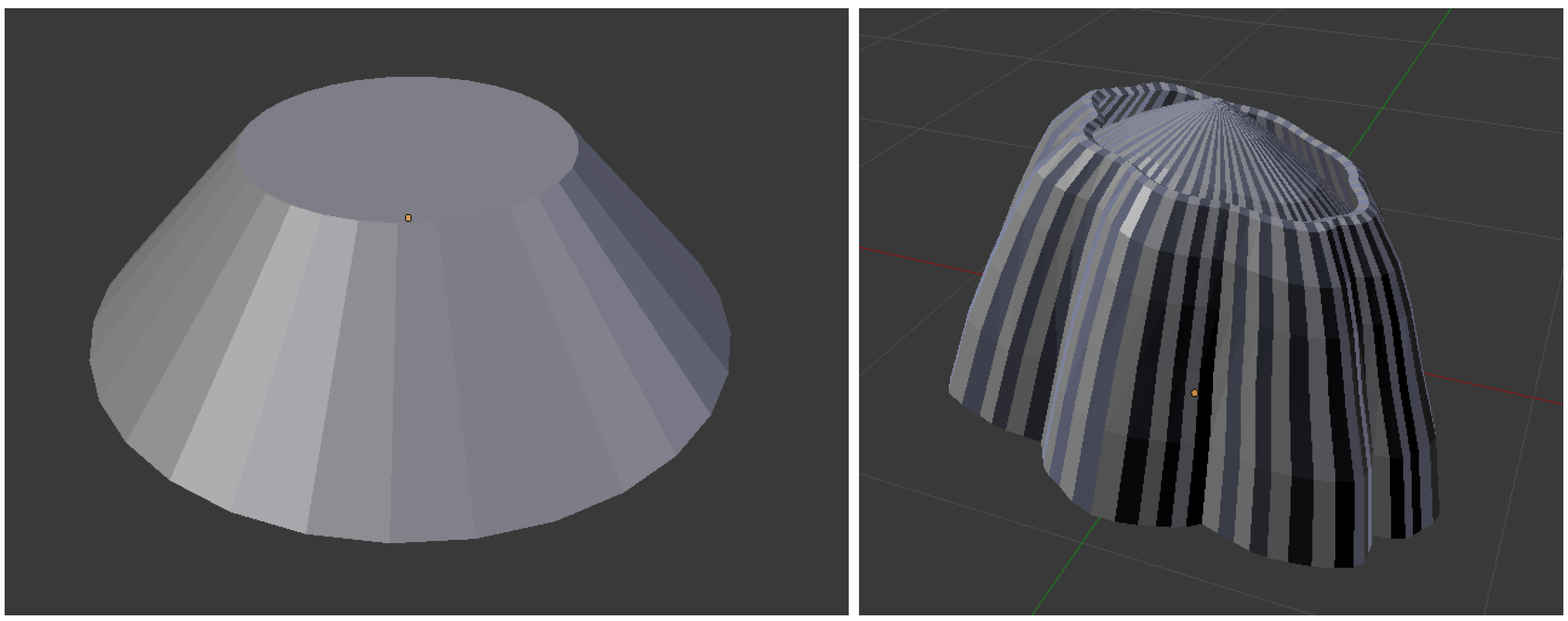
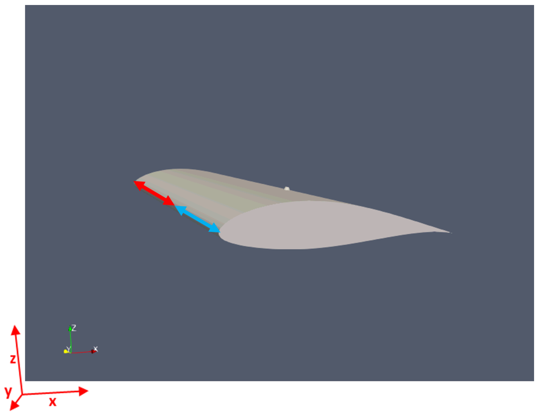
2.4.1. Motionless Blade Simulation with a Single Barnacle

The blade structure made for this test is identical to that of the original experimental study [13]. This allows us to work on the validation of the full-scale model. The foil section is a 55 mm chord NACA 63-619. The barnacle is also placed at 60% of the chord at 40 mm from the centre of the blade in the y direction. The barnacle is thus located at 1/4 of the length of the blade. Half of the blade is used as a reference (clean blade), and the barnacle is placed in the middle of the second part of the blade (Figure 2). The experimental data show that the impact of the barnacle on the blade is limited to a few barnacle base diameters (0.3 c) around the barnacle. Thus, the barnacle should not impact the results of the clean part of the computational domain. Both barnacle geometries are tested and compared.

Several sizes of computational domains were tested to remove the effects caused by boundary conditions for the smaller domain. Widths from 2 c to 8 c were tested and, after 3 c (1.65 m), numerical results were independent of the width. Thus the simulation channel is 1.60 m high × 8 m wide × 7.3 m long and limits the impact of the boundary conditions. The thinnest cells are located close to the blade walls to capture the boundary layer. The dimensionless wall distance, $y+$ is set to 1 on the clean section (${\displaystyle y+=\frac{y{u}_{\tau }}{\nu }}$, where y is the distance to the wall and $u_{\tau }$ is the friction velocity). Mesh is structured near the blade in six successive layers with an increase ratio of 1.3 between each layer. The wake expected position is refined using a refinement box to avoid the filtering by the mesh of the wake vortices. The refined mesh is shown in Figure 3. Irregularities on the 2D cut are due to 2D projections in 3D cells which are not distorted. The fluid used in motionless blade simulation is air (supposedly incompressible). The physical simulation parameters are given in

Table 2. Summary of the physical parameters used in simulations of the motionless blade cases.

Parameter	Value	Unit
ρ	1.177	kg·m−3
ν	1.57 × 10−5	m2·s−1
U∞	45	m·s−1
p∞	1.013 × 106	Pa
k	1.898	m2·s−2
ω	4.574	s−1

.

Four angles of attack were tested and compared to experimental data (5°, 10°, 14°, 15°). The Reynolds number of the motionless blade cases (with the chord (c = 0.055 m) as reference length) is $R{e}_c=1.5\times {10}^5$.

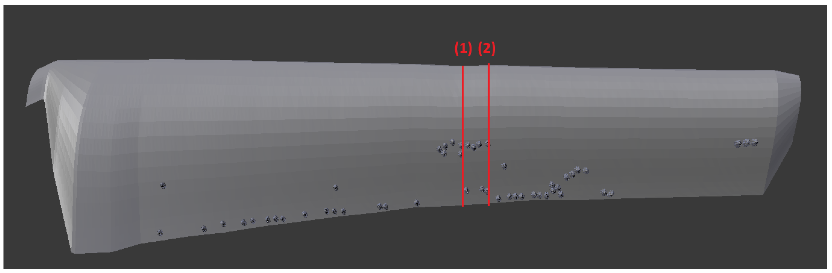
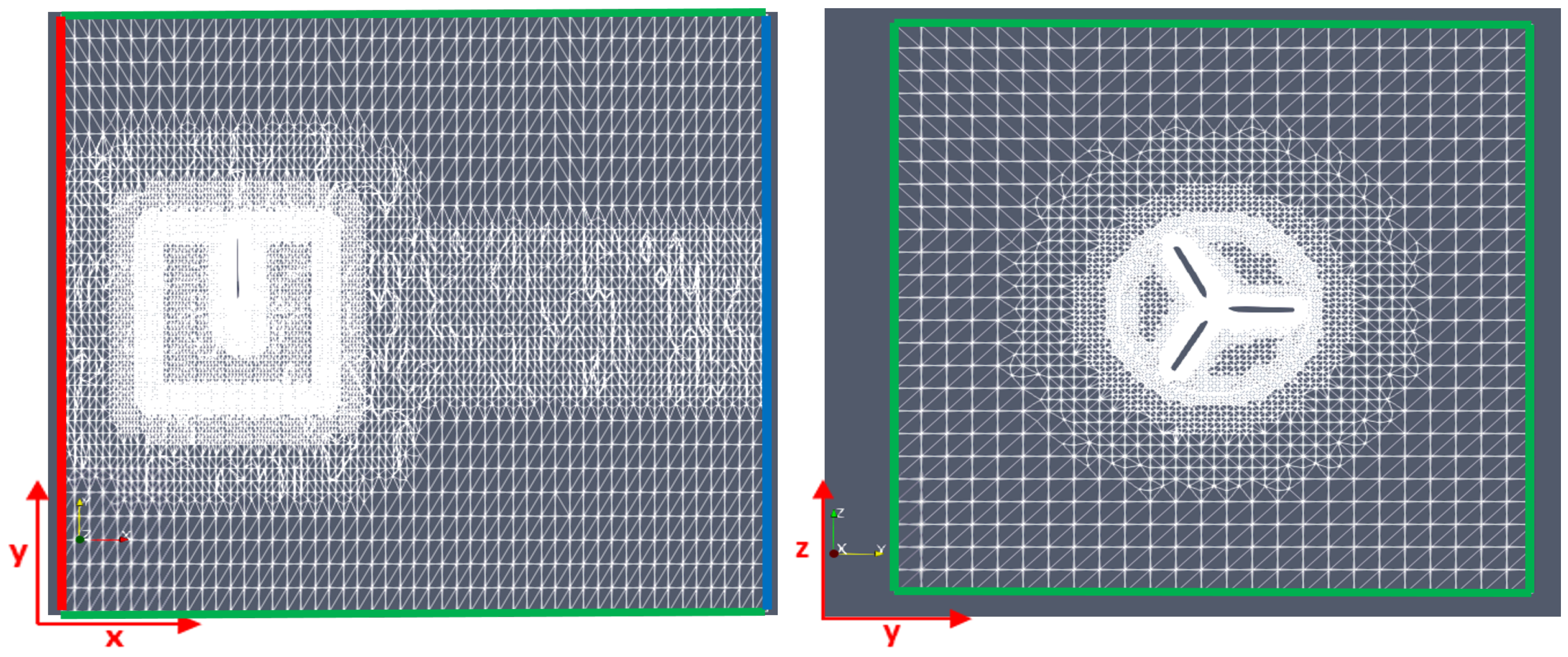
2.4.2. Full Rotor Simulation with a Realistic Barnacle Colonisation

In this section, a full rotor simulation is presented. The rotor hub is removed to limit the computation time. The turbine used in this work has been numerically studied previously for other subjects than biofouling (e.g., flow induced rotation) with clean blades [23]. Barnacles are fixed to the blades according to the realistic implantation on the blades of the AHH HS 1000 tidal turbine shown in [13] (Figure 4). We assume that the colonisation is identical on the three blades. The barnacles are settled on the downstream part of the blade, from 60% of the chord. Moreover, a large part of them are grouped in a patch. Indeed, the barnacles seem to favour the less energetic positions of the blades and their grouping contributes to protect them from the strongest currents. The chosen mesh for the clean case is the converged one used in [23]. It has been subjected to a mesh convergence study related to the forces applied to the rotor. For the fouled case, the general parameters of the mesh are kept, and the barnacles are taken into account as part of the solid structures. The computational domain is a cube with sides equal to 4 rotor diameters. The cells are twice as thin in the X-direction, which is the direction of the main velocity. Both meshes (clean and fouled) are composed of about 9 million points. Around the turbine, a 1.5 diameter refinement cylinder forms a moving part of the mesh. It is connected to the static zone by an Arbitrary Mesh Interface (AMI) which transfers fluid information from one zone to the other. The rotation of this cylinder generates the rotation of the rotor by sliding on the static zone. The mesh is shown in Figure 5.

The full rotor is moving in the water. Physical and numerical parameters are given in

Table 3. Summary of the physical parameters used in dynamic simulations of the rotor.

Parameter	Value	Unit
ρ	1025	kg·m−3
ν	1.3 × 10−6	m2·s−1
U∞	0.8	m·s−1
p∞	0	Pa
ΩR	9.143	rad·s−1
I∞	0.03	-

.

${\Omega }_R$ is the rotor’s rotation speed and $I_{\infty }$ is the turbulence intensity. The chord-based Reynolds number at the tip of the blades for the full rotor simulations is $R{e}_c=1.7\times {10}^5$.

2.5. Test Case Summary

Four simulations were run for the single blade case with a single barnacle for four angles of incidence (5°, 10°, 14° and 15°). Two simulations were run with the full rotor rotating structure: one with clean blades and one with a realistic colonisation of barnacles. To help distinguish the various configurations described above, the

Table 4. Summary of the numerical cases.

Case Name	Fluid	Rotation	Barnacle	Angle of Attack
Blade 5°	Air	No	Only one	5°
Blade 10°	Air	No	Only one	10°
Blade 14°	Air	No	Only one	14°
Blade 15°	Air	No	Only one	15°
Rotor clean	Water	Yes	Realistic	0°
Rotor colonised	Water	Yes	Realistic	0°

and

Table 5. Numerical parameters summary.

Case Name	ΔTmin (s)	ΔTmin (s)	ΔXmin (m)	Total Running Time
Blade 5°	∼10−7	∼10−4	$2.2\times {10}^{-4}$	1.26
Blade 10°	∼10−7	∼10−4	$2.2\times {10}^{-4}$	1.21
Blade 14°	∼10−7	∼10−4	$2.2\times {10}^{-4}$	1.16
Blade 15°	∼10−7	∼10−4	$2.2\times {10}^{-4}$	1.15
Rotor clean	∼10−9	∼10−4	$4.4\times {10}^{-4}$	2.41
Rotor colonised	∼10−12	∼10−4	$2.6\times {10}^{-4}$	1.505

provide a summary of the various cases and give some additional numerical parameters.

3. Results

This section is separated into two parts. Section 3.1 refers to the validation and comparison of the models with the experimental data with a single blade with only one barnacle on it. It is completed by a short analysis of the wake. Section 3.2 presents the comparison of two simulations with a rotor. The first simulation is the reference case with clean blades (the results are compared to experimental data) and the second is the case with a realistic colonisation (Figure 4).

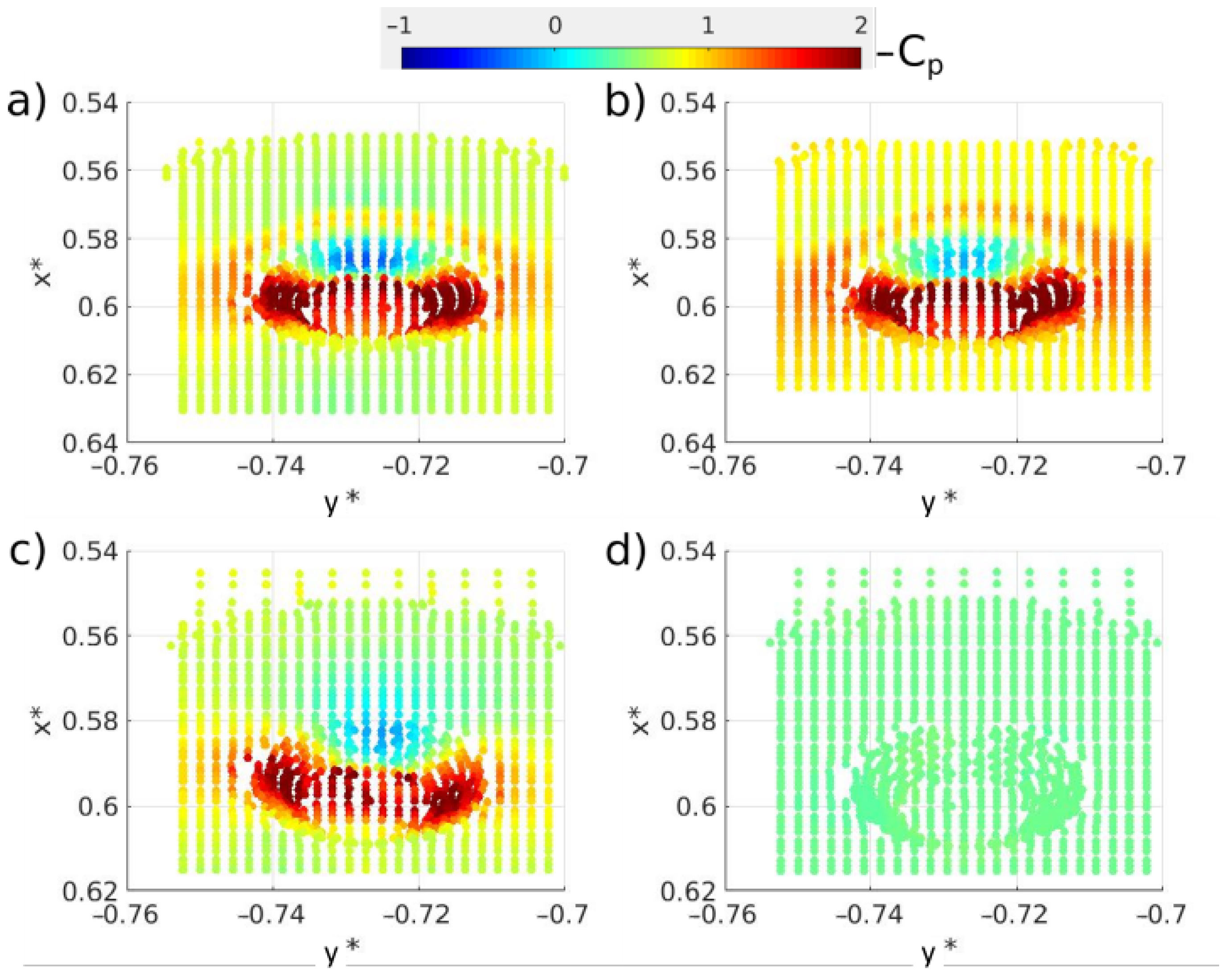
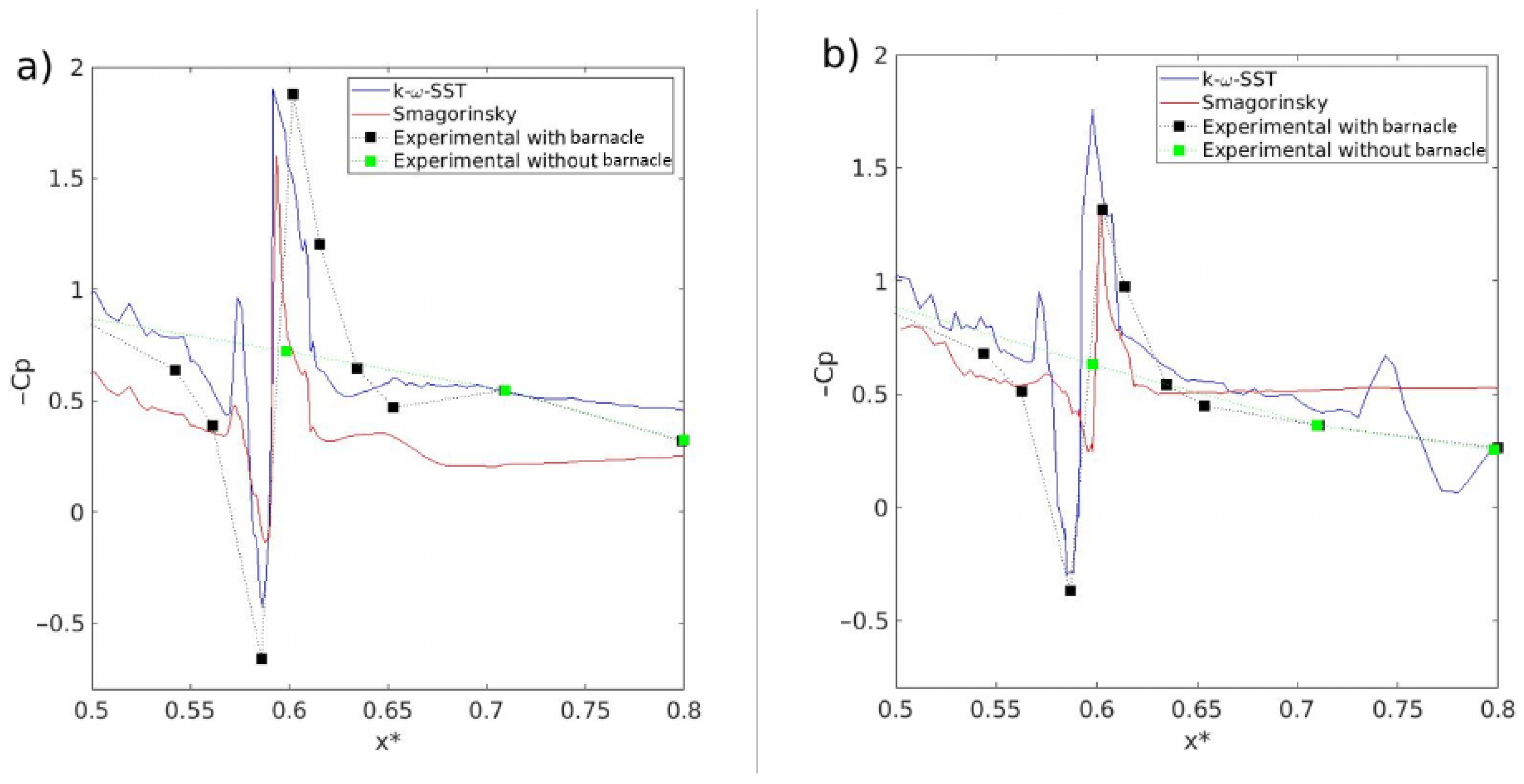
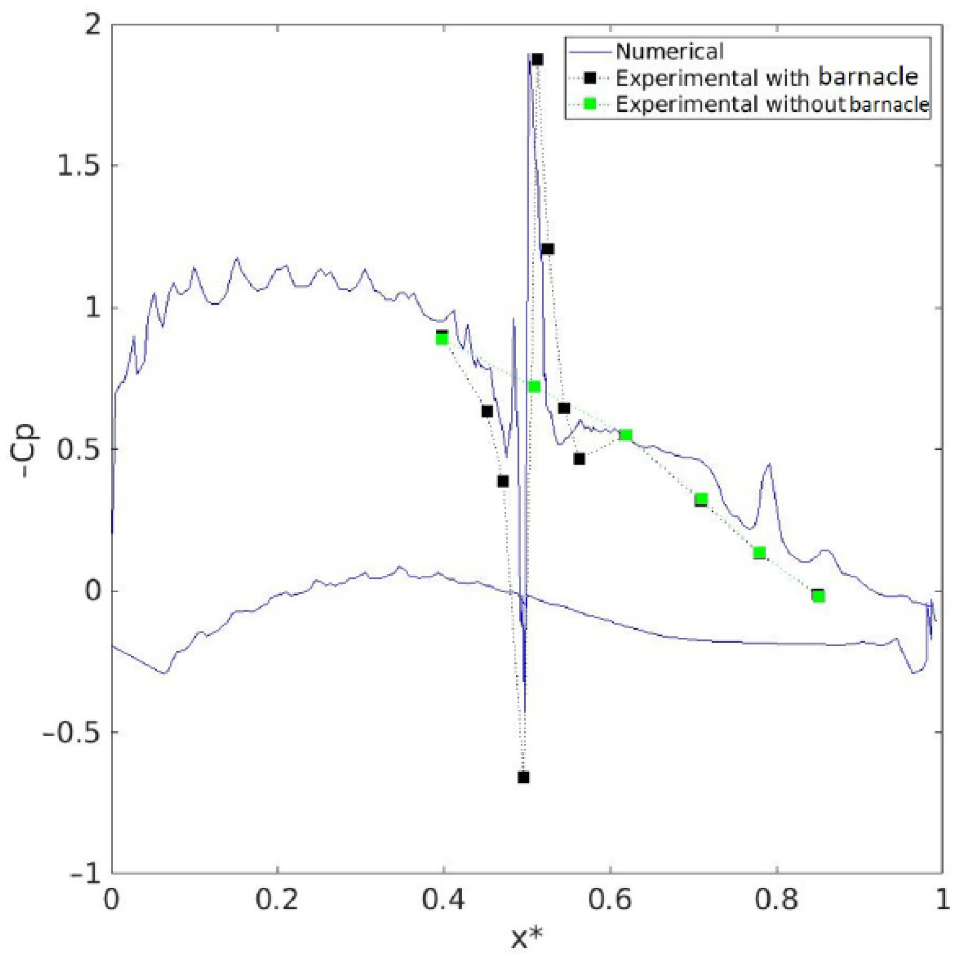
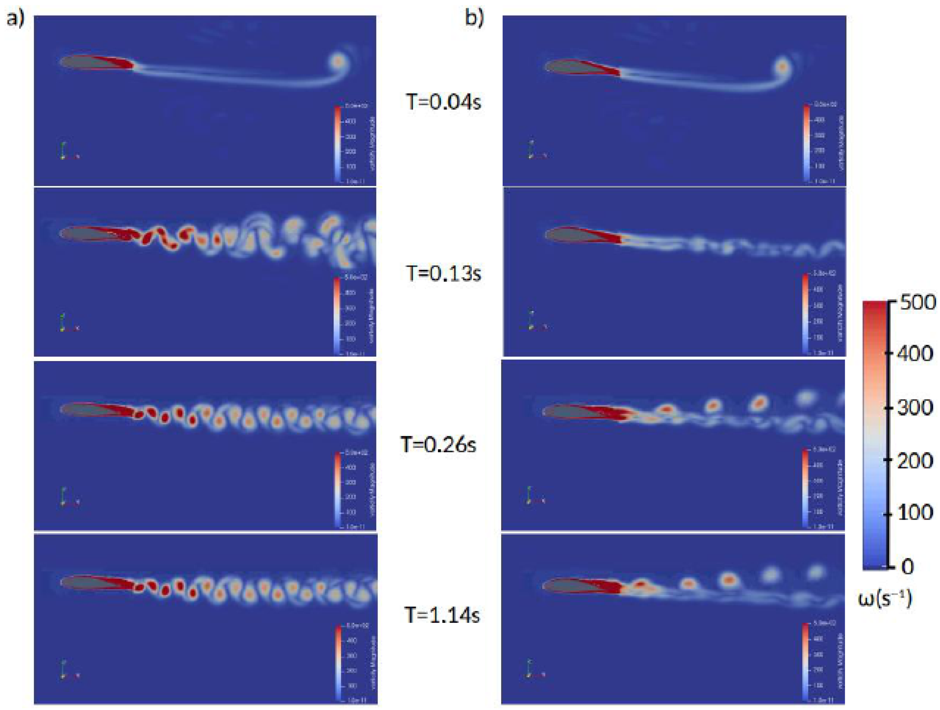
3.1. Motionless Blade Simulation with One Barnacle

To compare the numerical model results to experimental data, the pressure field around the barnacles is taken at every fluid cell centre (along the blade surface) in the studied area at fixed time points chosen after the flow stabilisation. On Figure 6 is presented the opposite of the pressure coefficient $C_p$ given by ${\displaystyle -C_p=\frac{p-p_{\infty }}{-q}}$, with $q=0.5\rho U_{\infty }^2=1191.71\mathrm{Pa}$. $X^{*}$ is the scaled position as $X^{*}=(x/c,y/c,z/c)=(x^{*},y^{*},z^{*})$, where x, y and z are, respectively, the stream-wise, the span-wise and the vertical directions. Nevertheless, with the LES model, results are not averaged, which explains slight asymmetries on pressure fields (Figure 6). The blade curvature is suppressed by projecting all the cells in a plane parallel to the blade mean angle. The mesh is refined around the complex geometries and the shape of the barnacle appears in the field extraction process.

The effects of the numerical conic barnacle are very similar to the experimental ones (Figure 6) (experimental pressure fields are available in [13]): in all cases, the barnacle is preceded by an over-pressure followed by a strong depression at the top of it. The flow change extends further downstream (3 radii) than upstream (2 radii). On the sides, the impact is felt up to 4 radii. Even with a numerical model, the perfect symmetry of the results is not guaranteed because the turbulence of the fluid creates slight variations in the flow that impact the distribution of the fluid pressure near the wall. The orders of magnitude of the $C_p$ coefficient are the same as those measured experimentally. The main value in the field is 5.2% higher in the numerical results. The effect of the angle of attack on the pressure field is consistent with measurements: the higher the angle, the smaller the biofouling effect. The pressure field is almost unchanged for an angle of attack of 15°.

To represent better the scales of the pressure variation and compare the models, the evolution of the opposite of $C_p$ along the chord is plotted in Figure 7. The two models present different behaviours downstream of the barnacle. The k-ω SST model is better for the lowest angle of attack (5°), with the pressure increasing progressively along the chord as in the experimental data until it reaches its final value at the trailing edge. In contrast, the Smagorinsky model overestimates the pressure field which tends to decrease behind the barnacle. However, both turbulence models allow a good reproduction of the pressure drop in the fouling area.

With the 10° angle, the two turbulence models are closer in terms of mean value. However, the k-ω SST model better represents the overpressure in front of the barnacle. Downstream, both models underestimate the pressure along the blade.

The modelling is less accurate for 15°. Indeed, both turbulence models underestimate the impact of the barnacle on the flow. An additional computation is then performed to study the behaviour of the model in this critical range of values (Figure 8). At 14°, the simulated impact is more coherent with the measurements but some discrepancies are observed. We deduced that the experiment is highly sensitive to the angle of attack in the range between 14° and 15°. Small variations in the experiment or the 3D geometry can also interfere with results.

Numerical simulation ensures a full $C_p$ profile along the blade without having to invest in additional probes (Figure 9). For example, the small decrease in pressure before the overpressure ($0.56<x^{*}<0.57$) was not captured by the probes during the experimental session. This phenomenon only appears for low angles (up to 10°). Normal (${\displaystyle C_n=\frac{n}{q}}$, where n is the forces normal to the blade per unit of span) and drag (${\displaystyle C_d=\frac{d}{q}}$, where d is the pressure drag forces of the blade per unit of span) coefficients are computed (Figure 10). As shown in experimental data, the barnacle has no significant impact on $C_n$. The coefficient grows until it reaches the aerodynamic stall around 13° before decreasing with the angle. The drag coefficient is more impacted by the barnacle with an exponential increase for a mean angle greater than 10°. The barnacle causes an increase in this coefficient for low mean angles. However, when the angle continues to increase, the dynamic stall becomes more important and the effect of the barnacle fades. The numerical model reproduces this tendency. For the angle of attack of 15°, the pressure variations caused by the barnacle are almost zero. The simulation then shows results close to those expected for a clean blade. The experimental data still show an impact for this angle but the numerical results at 14° overestimate these variations. Thus, the model seems very sensitive to the angle of attack parameter.

The main difference between the two turbulence models is their ability to compute the wake. Figure 11 shows that the LES successfully separates the vortex releases from each other. The RANS model, which averages the physical quantities, only identifies the general shape of the wake. The intensity of the vortexes is also lower, indicating a higher numerical dissipation. Thus, the LES is chosen over the RANS for its better ability to represent the wake.

Figure 12 compares the time evolution of the wake of the clean part of the blade with the one in the plane of the barnacle with an angle of attack of 5°. In both cases, the first vortex is identical (T = 0.4 s) but, while the clean case starts to stabilise quickly with vortex releases alternating between the lower and upper surface, the barnacle case does not show vortexes of high vorticity intensity (>300 s⁻¹) during the first time steps. Once the wake is stabilised, the biofouling blade releases vortexes that propagate “upwards” in a regular manner. The clean blade, on the other hand, shows a turbulence structure similar to Von Karman vortex streets.

Finally, the wake thickness is an interesting physical quantity to analyse: Figure 13 shows, as expected, that for the case without a barnacle as well as for the case with a barnacle, the wake thickness increases with the distance behind the blade. However, the behaviour of this increase is not the same in both cases. In the clean case, the increase is slower and follows a parabolic trend, while the case with the barnacle shows a faster and linear increase. Off the finer part of the mesh shown in Figure 3 which extends 4 chords downstream of the blade, the mesh is too coarse and diffuses the vortexes too quickly to follow the evolution of the wake thickness. It would be interesting to know if, further downstream, the wake thickness of the case without a barnacle eventually catches up with the one of the case with a barnacle.

3.2. Full Rotor Simulation Simulation

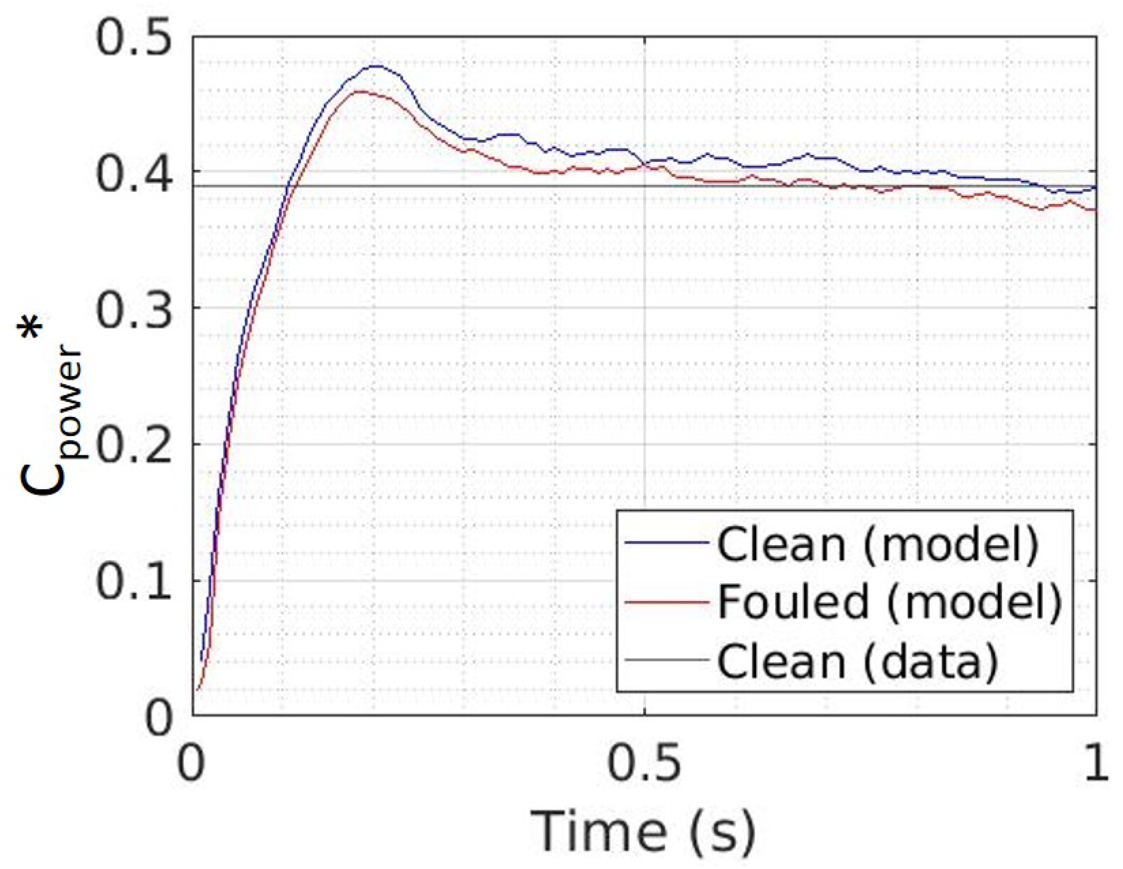
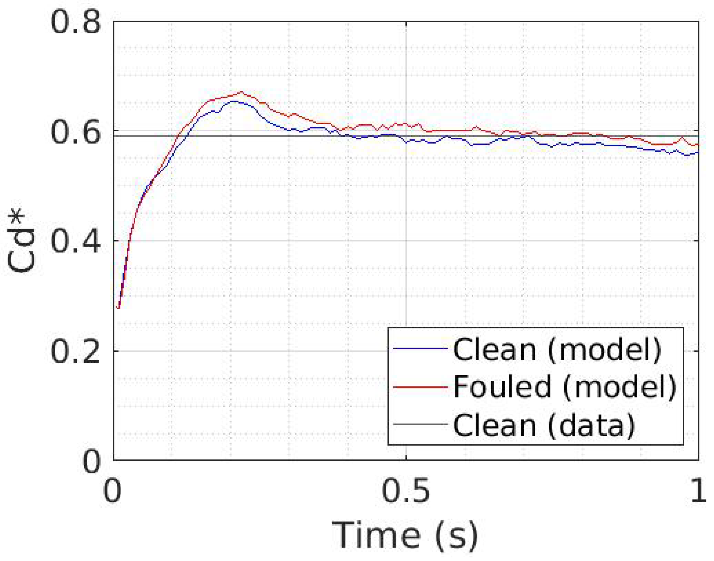
3.2.1. Impact of Biofouling on Tidal Turbine Performances

The time evolution of the power and drag coefficients ($C_{power}$ and $C_d$) for the complete rotor are shown in Figure 14 and Figure 15. The realistic addition of the sessile species, according to [13], does not change the general behaviour of the turbine. However, a decrease in $C_{power}$ by 1.6% is observed. It is explained by an early dynamic stall and the formation of re-circulation loops on the upper surface. However, under the chosen conditions, the barnacles do not seem to create any additional boundary layer stall, which transitions by itself relatively close to the leading edge This can be explained by the particular position of the barnacles: the individuals naturally fix themselves in a zone that is already less energetic, where it is easier to settle. This small drop of $C_{power}$ may also be related to the small area colonised. If the blade was more fouled, with larger or more numerous species, the result might be more significant. In any case, the difference of the pressure coefficient is not sufficient to conclude to a performance loss.

The drag coefficient increases by 7.5% (Figure 15). It is significantly less than for the motionless blade case simulation that reached a rising of 800% for low angles of attack. This result can be explained by two points. Barnacles do not take part in the dynamic stall, contrary to the motionless blade case where the barnacle is located at 60% of the chord. Then, the barnacles are not evenly distributed on the blade and remain relatively far from each other. 3D effects also play a role in the process: the vortexes generated by the more upstream barnacles are not directly sent into the wake as in 2D but continue to follow the blade on a different plane from the barnacle.

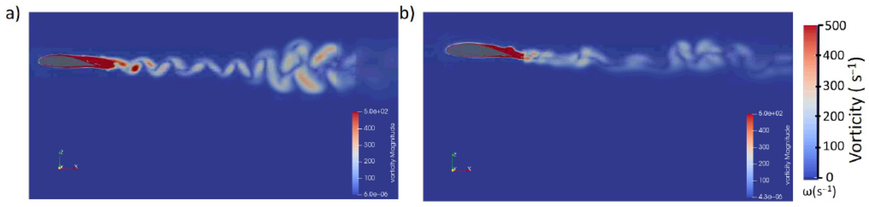
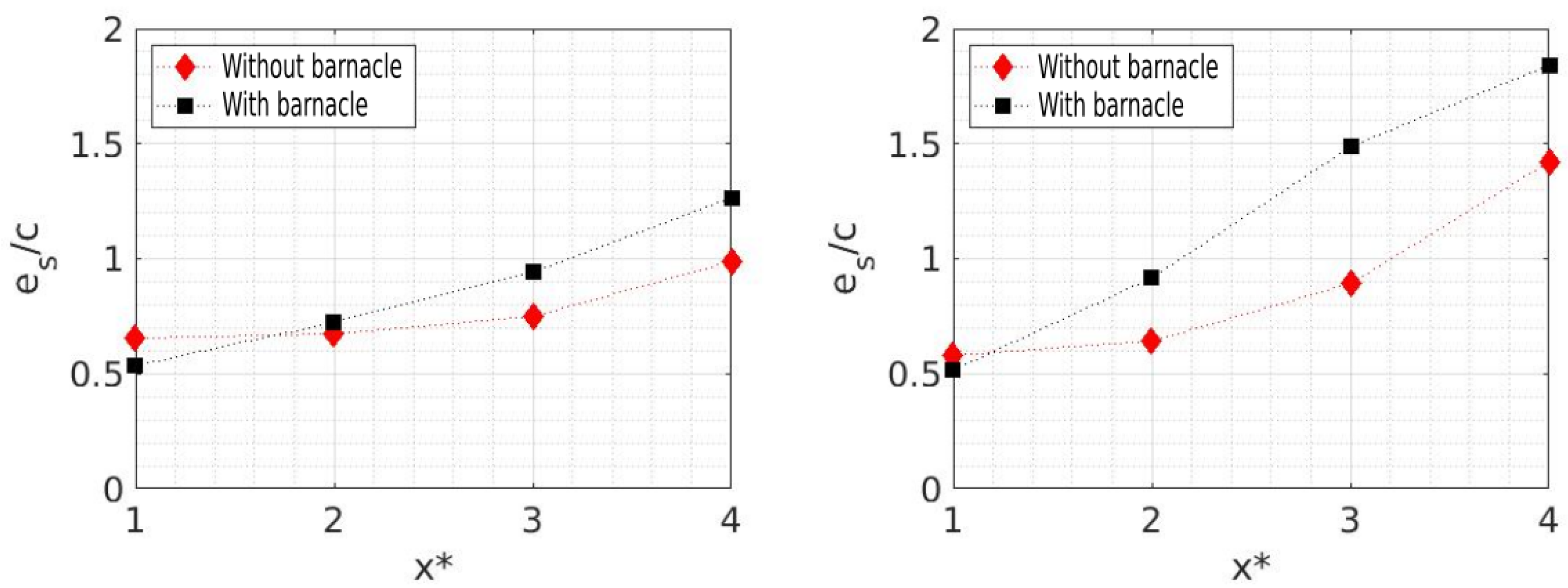
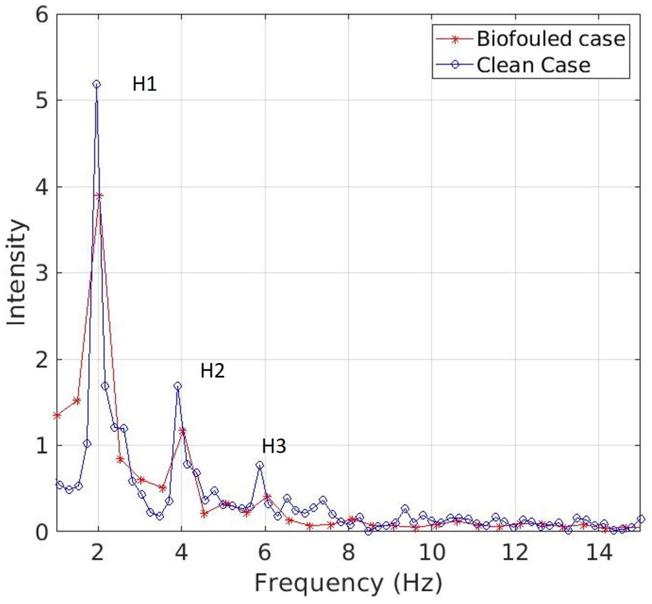
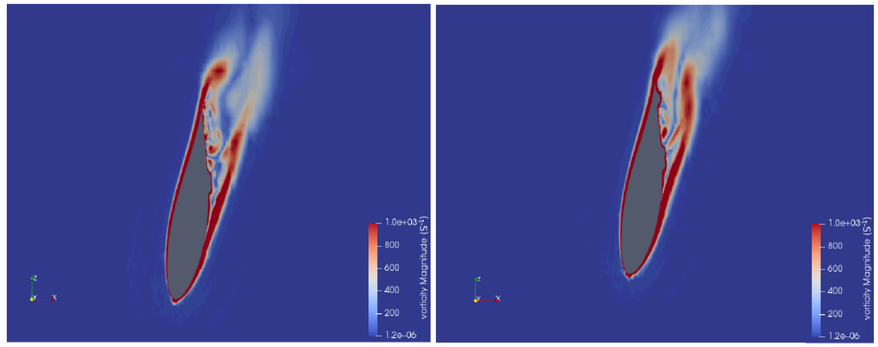
3.2.2. Impact of Biofouling on Tidal Turbine Wake

The chosen configuration does not allow us to see any significant impact of the colonisation on the wake of the tidal turbine. The fluid–structure interactions generated by the barnacles are small and are therefore quickly diffused and dissipated. The isovalues of the Q criteria show no significant differences in the wake or near wall. Nevertheless, a probe is placed downstream (1 diameter) of the turbine at the tip of the blade position (0.7, 0.35, 0) to study pressure, velocity and vorticity variations. The signals are relatively close for the clean and fouled cases. The amplitude of vorticity magnitude variation is lower in the biofouled case than in the clean one. The curve is also less smooth: showing that small vortexes regularly pass in the wake. A Discrete Fourier Transform (DFT) analysis of the vorticity signal is performed over 1.2 s with a time step of 0.005 s (240 samples) (Figure 16). The sample is one second long on the same time period for both cases. Both signals show a main harmonic around 2 Hz that corresponds to the tip vortex releases of the turbine. The intensity of the main harmonic (H1) is lower in the biofouled case than in the clean case. The first three harmonics are also slightly shifted (0.1 Hz) towards the high frequencies and less intense than in the clean case. In general, biofouling leads to an energetic decrease in the vortexes generated by the colonised surfaces.

A zoomed view of the blades allows us to understand how barnacles act on fluid to generate these vortexes (Figure 17). These figures confirm the fact that barnacles are behind the boundary layer transition. Nevertheless, in the case of a single barnacle, the vortexes generated by the fouling are directly sent downstream whereas in presence of a second barnacle in the same plan, the vortexes remain blocked between the two barnacles. The recirculation loop acts as a new surface over which the fluid flows. This shows that a single barnacle can have more effect on the wake than a couple in the same plane.

4. Discussion and Conclusions

The three-dimensional study of explicit roughness raises difficult issues. The authors are aware that, despite the good results for the total forces, the pressure profiles shown in Figure 7, Figure 8 and Figure 9, denote a non-physical behaviour (especially at the leading edge) even when averaged over time. This issue could perhaps be fixed using a finer mesh around the blade in the uniform straight flow. A mesh convergence study should therefore be carried out to overcome the issue.

For the full rotor, the authors were strongly constrained by the computational facilities. The mesh convergence was ensured by a preliminary study [23]. The numerical stability for the converged mesh requires very small time steps reaching (${10}^{-12}$ s). Thus, the simulations could only achieve three rotations in the clean case and two for the biofouled case. This produces drag and power coefficients which converge to a constant value, which allows us to conclude that the simulation is valid concerning the forces. However, the simulation time is too short to study a realistic behaviour of the wake, especially for the biofouled case. The DFT gives interesting results but should be performed on a longer time period.

The Reynolds number is also constant for the motionless blade and the full rotor simulations (around $1.6\times {10}^5$). A full scale turbine could have a higher $Re$ in a realistic configuration. The increase in the $Re$ would correspond to an increase in flow velocity relative to the blade profiles. However, experimental data from the motionless blade tends to show that the sooner the stall occurs, the less impact the biofouling has. The tests presented here may overestimate the actual losses due to biofouling.

This paper presents a numerical analysis of the impact of biofouling on turbines performances. Two turbulence models are compared to know which is the more suitable here. k-ω SST is better at predicting forces on the blade in the motionless blade cases (Figure 7 and Figure 8) but the Smagorinsky model was used for the full rotor because of its capacity to compute the wake with accuracy (Figure 11).

Conclusions on the impact of biofouling on tidal turbines performances are close to the experimental results: for the motionless blade case, the barnacle does not impact the normal forces but highly increases the drag, especially for low mean angles. This phenomenon decreases when the angle continues to rise because of the natural stall of the profile that occurs upstream of the barnacle (Figure 6, Figure 7 and Figure 8). No significant differences are noted between the conical and realistic barnacle structures. It is therefore recommended to work with the simplest model. A dynamic simulation of a full scale rotor is also performed with a realistic colonisation. Barnacles tend to be placed on the second part of the chord where the hydrodynamic stall creates a less energetic zone. This has the effect of greatly reducing their impact on the performance of the tidal turbine, which only loses less than 1% of its efficiency. The impact of the biofouling on the tidal turbine performance is clearly reduced in the full rotor case (Figure 14 and Figure 15). First of all, the realistic position of barnacles (mostly in the second part of the chord) plays an important role on this result. Then, the fouled surface remains relatively low compared to the blade’s surfaces. Lastly, the turbulence is quite different in the full rotor case; the blades generate big vortexes that propagate and possibly impact with the others. This increase in turbulence may be one of the reasons for the drop in the impact of the biofouling in realistic configurations. However, regardless of their position, biofouling generates drag (Figure 10 and Figure 15). In the wake, the vortexes created by the biofouled structures are less energetic and diffuse more quickly (Figure 13 and Figure 16). This phenomenon could even be advantageous for tidal farms where it is important that the downstream tidal turbines suffer little disturbance from the upstream tidal turbines in order to avoid rapid fatigue of the installations and a significant loss of production. However, it is important to remember that, although this is a realistic layout, there are as many configurations as there are geographical areas and therefore as many sessile species. Erect Hydrozoans that are not robust could have far greater effects than those highlighted here. More extensive colonisation could also change our results. Other implantation scenarios should now be explored. A characterisation and parametrisation of the biofouling will be considered to estimate the impact of the biofouling at different scale and development phases.

References

1. Vinagre, P.A.; Simas, T.; Cruz, E.; Pinori, E.; Svenson, J. Marine Biofouling: A European Database for the Marine Renewable Energy Sector. J. Mar. Sci. Eng. 2020, 8, 495. [Google Scholar] [CrossRef]
2. Titah-Benbouzid, H.; Benbouzid, M. Marine Renewable Energy Converters Biofouling: A Critical Review on Impacts and Prevention. In Proceedings of the EWTEC, Nantes, France, 6–11 September 2015; pp. 1–8. [Google Scholar]
3. Kerr, A.; Beveridge, C.; Cowling, M.; Hodgkiess, T.; Parr, A.; Smith, M. Some physical factors affecting the accumulation of biofouling. J. Mar. Biol. Assoc. UK 1999, 79, 357–359. [Google Scholar] [CrossRef]
4. Foveau, A.; Dauvin, J.C. Surprisingly diversified macrofauna in mobile gravels and pebbles from high-energy hydrodynamic environment of the ‘Raz Blanchard’ (English Channel). Reg. Stud. Mar. Sci. 2017, 16, 188–197. [Google Scholar] [CrossRef] [Green Version]
5. Raoux, A.; Tecchio, S.; Pezy, J.; Lassalle, G.; Degraer, S.; Wilhelmsson, D.; Cachera, M.; Ernande, B.; Le Guen, C.; Haraldsson, M.; et al. Benthic and fish aggregation inside an offshore wind farm: Which effects on the trophic web functioning? Ecol. Indic. 2017, 72, 33–46. [Google Scholar] [CrossRef] [Green Version]
6. Lindholdt, A.; Dam-Johansen, K.; Olsen, S.; Yebra, D.; Kiil, S. Effects of biofouling development on drag forces of hull coatings for ocean-going ships: A review. J. Coat. Technol. Res. 2015, 12, 415–444. [Google Scholar] [CrossRef]
7. Song, S.; Ravenna, R.; Dai, S.; DeMarco Muscat-Fenech, C.; Tani, G.; Kemal Demirel, Y.; Atlar, M.; Day, S.; Incecik, A. Experimental investigation on the effect of heterogeneous hull roughness on ship resistance. Ocean Eng. 2021, 223, 108590. [Google Scholar] [CrossRef]
8. Heechan, J.; Seung Woo, L.; Seung Jin, S. Measurement of Transitional Surface Roughness Effects on Flat-Plate Boundary Layer Transition. ASME J. Fluid Eng. 2019, 141, 074501. [Google Scholar]
9. Balachandar, R.; Blakely, D. Surface roughness effects on turbulent boundary layers on a flat plate located in an open channel. J. Hydraul. Res. 2004, 42, 247–261. [Google Scholar] [CrossRef]
10. Chakroun, W.; Al-Mesri, I.; Al-Fahad, S. Effect of Surface Roughness on the Aerodynamic Characteristics of a Symmetrical Airfoil. Wind Eng. 2004, 28, 547–564. [Google Scholar] [CrossRef]
11. Gholamhosein, S.; Mirzaei, M.; Nazemi, M.M.; Fouladi, M.; Doostmahmoudi, A. Experimental study of ice accretion effects on aerodynamic performance of an NACA 23012 airfoil. Chin. J. Aeronaut. 2016, 29, 585–595. [Google Scholar]
12. Orme, J.; Masters, I.; Griffiths, R. Investigation of the effects of the biofouling on the efficiency of marine current turbines. In Proceedings of the MAREC2001,International Conference of Marine Renewable Energies, London, UK, 27–28 March 2001; pp. 91–99. [Google Scholar]
13. Walker, J.; Green, R.; Gillies, E.; Phillips, C. The effect of a barnacle-shaped excrescence on the hydrodynamic performance of a tidal turbine blade section. Ocean Eng. 2020, 217, 107849. [Google Scholar] [CrossRef]
14. Rivier, A.; Bennis, A.C.; Jean, G.; Dauvin, J.C. Numerical simulations of biofouling effects on the tidal turbine hydrodynamic. Int. Mar. Energy J. 2018, 1, 101–109. [Google Scholar] [CrossRef]
15. Picioreanu, C.; Vrouwenvelder, J.H.; van Loosdrecht, M. Three-dimensional modeling of biofouling and fluid dynamics in feed spacer channels of membrane devices. J. Membr. Sci. 2009, 345, 340–354. [Google Scholar] [CrossRef]
16. Demirel, Y.K.; Turan, O.; Incecik, A. Predicting the effect of biofouling on ship resistance using CFD. Appl. Ocean Res. 2017, 62, 100–118. [Google Scholar] [CrossRef] [Green Version]
17. Song, S.; Shi, W.; Demirel, Y.K.; Atlar, M. The effect of biofouling on the tidal turbine performance. In Applied Energy Symposium; MIT: Cambridge, MA, USA, 2019; pp. 1–10. [Google Scholar]
18. Mycek, P. Numerical and Experimental Study of the Behaviour of Marine Current Turbines. Ph.D. Thesis, University of Le Havre, Le Havre, France, 2013. (In French). [Google Scholar]
19. Greenshields, C. OpenFoam User Guide Version 6; OpenFOAM Foundation: London, UK, 2018. [Google Scholar]
20. Ramirez-Pastran, J.; Duque-Daza, C. On the prediction capabilities of two SGS models for large-eddy simulations of turbulent incompressible wall-bounded flows in OpenFOAM. Cogent Eng. 2019, 6, 1679067. [Google Scholar] [CrossRef]
21. Marten, D.; Peukert, J.; Pechlivanoglou, G.; Nayeri, C.; Paschereit, C. QBLADE: An Open Source Tool for Design and Simulation of Horizontal and Vertical Axis Wind Turbines. Int. J. Emerg. Technol. Adv. Eng. 2013, 3, 264–269. [Google Scholar]
22. Community, B.O. Blender-a 3D Modelling and Rendering Package; Blender Foundation, Stichting Blender Foundation: Amsterdam, The Netherlands, 2018. [Google Scholar]
23. Robin, I.; Bennis, A.C.; Dauvin, J.C. 3D Simulation with Flow-Induced Rotation for Non-Deformable Tidal Turbines. J. Mar. Sci. Eng. 2021, 9, 250. [Google Scholar] [CrossRef]
Figure 1. 3D structures of the conic (left) and realistic (right) barnacles.
Jmse 09 01288 g001
Figure 2. 3D geometry of the blade with one barnacle. The clean part of the blade is marked by the red arrow. The barnacle is in the middle of the section marked with the blue arrow.
Jmse 09 01288 g002
Figure 3. 3D geometry and mesh of the entire computational domain (a), around the blade (b), and around the conic barnacles (c). Distored cells are due to the cutting plane and do not represent the 3D cells.
Jmse 09 01288 g003
Figure 4. 3D geometry of one of the three blades of the rotor with barnacles. Red lines are cut positions for post-processing.
Jmse 09 01288 g004
Figure 5. Views of the X–Y (left) and Y–Z (right) planes of the computational domain including the rotor geometry. Green lines are the no-slip boundary conditions, the red line is the inlet with the velocity condition and the blue line is the pressure outlet condition.
Jmse 09 01288 g005
Figure 6. Opposite of the pressure coefficient ( C p ) around barnacle for an angle of attack of 5° (a), 10° (b), 14° (c) and 15° (d) on the blade surface. Results are from LES simulation.
Jmse 09 01288 g006
Figure 7. Opposite Pressure coefficient evolution ( C p ) according to the dimensionless x position ( x * ) along the chord-wise position on the centre-line for an angle of attack of 5° (a) and 10° (b). Numerical results with k-ω SST (blue line) and Smagoginsky (red line) are presented for the fouled blade. Experimental values for clean and fouled blades are shown in green and black squares, respectively, from [13] data.
Jmse 09 01288 g007
Figure 8. Opposite Pressure coefficient ( C p ) evolution according to the dimensionless x position ( x * ) along the chord-wise position on the centre-line for an angle of attack of 15° (a) and 14° (b). Numerical results with k-ω SST (blue line) and Smagorinsky (red line) are presented for the fouled blade. Experimental values for clean and fouled blades are shown in green and black squares, respectively, (with an angle of attack of 15°) from [13] data.
Jmse 09 01288 g008
Figure 9. C p evolution against the dimensionless x-position profile (including the lower face) at a fixed time point for numerical modelling with fouling (blue line) and experimental mean values for a clean blade (green squares) and a fouled blade (black squares) for an angle of attack of 5° from [13] data.
Jmse 09 01288 g009
Figure 10. Normal (Left) and drag (Right) coefficients measurements against the mean angle for clean (black squares) and fouled (green crosses) blades from [13] data. Numerical results for fouled blades are represented by red lozenges.
Jmse 09 01288 g010
Figure 11. Magnitude of the vorticity around and behind the blade for the LES Smagorinsky (a) and the RANS k- ω SST turbulence model (b).
Jmse 09 01288 g011
Figure 12. Magnitude of vorticity around and behind the blade at T = 0.04 s, T = 0.13 s, T = 0.26 s, and T = 1.14 s for cases without (a) and with (b) a barnacle.
Jmse 09 01288 g012
Figure 13. Dimensionless wake thickness as a function of dimensionless position in the wake without (red diamonds) and with (black squares) a barnacle for angles of attack of 5° (left) and 15° (right).
Jmse 09 01288 g013
Figure 14. Time evolution of the corrected power coefficient ( C p o w e r * ). Measurements for a clean turbine are in black while numerical results for clean and fouled turbines are in blue and red, respectively.
Jmse 09 01288 g014
Figure 15. Same legend as for Figure 14 but for the corrected drag coefficient ( C d * ).
Jmse 09 01288 g015
Figure 16. Discrete Fourier Transform of the vorticity numerical magnitude took one diameter behind the rotor at the tip of the blade position for a clean (blue line) and fouled (red line) tidal turbine. The probe appears on Figure 5.
Jmse 09 01288 g016
Figure 17. Zoomed view of two sections of one blade of the tidal turbine in the X–Z plan. The left refers to (1) and the right section refers to (2) on Figure 5.
Jmse 09 01288 g017