Article

Scale-Resolving Simulations of a Circular Cylinder Subjected to Low Mach Number Turbulent Inflow

1
Maritime Research Institute Netherlands (MARIN), Haagsteeg 2, 6708 PM Wageningen, The Netherlands
2
Faculty of Mechanical, Maritime and Materials Engineering, Delft University of Technology, Mekelweg 5, 2628 CD Delft, The Netherlands
*
Author to whom correspondence should be addressed.
J. Mar. Sci. Eng. 2021, 9(11), 1274; https://doi.org/10.3390/jmse9111274
Submission received: 8 October 2021 / Revised: 9 November 2021 / Accepted: 12 November 2021 / Published: 16 November 2021
(This article belongs to the Section Ocean Engineering)

Abstract

:
Inflow turbulence is relevant for many engineering applications relating to noise generation, including aircraft wings, landing gears, and non-cavitating marine propellers. While modelling of this phenomenon is well-established for higher Mach number aerospace problems, lower Mach number applications, which include marine propellers, still lack validated numerical tools. For this purpose, simplified cases for which extensive measurement data are available can be used. This paper investigates the effect of inflow turbulence on a circular cylinder at a Reynolds number of 14,700, a Mach number of 0.029, and with inflow turbulence intensities ranging between 0% and 22%. In the present work focus is put on the hydrodynamics aspect, with the aim of addressing radiated noise in a later study. The flow is simulated using the partially averaged Navier Stokes equations, with turbulence inserted using a synthetic inflow turbulence generator. Results show that the proposed method can successfully replicate nearfield pressure variations and relevant flow features in the wake of the body. In agreement with the literature, increasing inflow turbulence intensity adds broadband frequency content to all the presented fluctuating flow quantities. In addition, the applied variations in inflow turbulence intensity result in a major shift in flow dynamics around a turbulence intensity of 15%, when the dominant effect of von Kármán vortices on the dominant flow dynamics becomes superseded by freestream turbulence.

1. Introduction

Turbulence-body interaction is a commonly occurring problem in engineering applications, particularly wings and propellers, and is of interest since it can lead to significant fluctuating forces and noise radiation. Examples of when inflow turbulence may be important are devices operating in geophysical turbulent flows, such as wind [1] and tidal turbines [2], or in the wake of an upstream body, such as a propeller behind a ship [3] or submarine hull [4]. Inflow turbulence noise is known to be the dominant low-frequency noise source for low Mach number aeroacoustic applications, including wind turbines [5], axial fans [6] and aircraft landing gear [7]. This is also the case for non-cavitating marine propellers, such as those of submarines.
The development and validation of numerical models for predicting inflow turbulence (IT) noise during design has a long history, from semi-analytical approaches [8] to advanced computational fluid dynamics (CFD) simulations [9]. Due to the physical complexity and high computational cost associated with inflow turbulence problems, simplified geometries are often preferred for these purposes, such as circular cylinders [10,11,12] and airfoils [9,13]. Nevertheless, these cases represent a challenge from a numerical point of view, due to the complex interaction of the inflow turbulence with the body’s leading edge and—in the case of the cylinder—the boundary layer and wake [14]. An appropriate treatment of these interactions is critical to accurately capture near- and farfield pressure predictions in simulations [15].
Furthermore, the need to resolve turbulence both upstream of and around the object of interest means that expensive scale-resolving simulations (SRS) are required. The challenges associated with performing this type of computation are summarised in [16]. Scale-resolving simulations are also essential for computing broadband noise sources directly from the computations. For problems with low Mach numbers, such as marine applications, the computational cost can be reduced by using an incompressible flow solver. A suitable method for generating representative inflow turbulence also needs to be applied [17]. For practical problems, consideration also needs to be given to effects of such factors like salinity and water temperature [18].
Our ultimate aim is to be able to provide robust and validated inflow turbulence noise predictions at conditions with low Mach numbers, something which is still limited to but a few studies in the literature (see, e.g., [19]). Before this can be achieved, it is necessary to validate the ability of the inflow turbulence generator to reproduce realistic inflow turbulence and correctly simulate the interactions of turbulence with complex flow around realistic geometries. To this end, the present study investigates the flow around a circular cylinder for which extensive experimental hydrodynamic validation data are available for several inflow turbulence intensities ( T I ) [11,12]. We also present results for inflow turbulence intensities above those measured, in order to further study the trends for high T I .

2. Methodology

2.1. Fluid Flow Solver

The governing flow equations were solved using an open-usage finite volume code, ReFRESCO, developed and maintained by MARIN (Maritime Research Institute Netherlands) in collaboration with various universities and institutions around the world [20]. The code uses unstructured spatial discretisation, allowing for high-quality structured grids to be used together with unstructured hexahedral grids that are easier to generate. Due to the necessity to resolve shear-layer instability, vortex shedding, inflow turbulence, and the turbulent wake of the cylinder, partially averaged Navier Stokes (PANS) modelling has been used.
In this methodology, the instantaneous quantities, Φ , are decomposed into a resolved, Φ , and a modelled (unresolved) component, ϕ , according to Φ = Φ + ϕ [21,22]. Applying this decomposition to the incompressible, single-phase, Newtonian mass conservation and Navier-Stokes equations leads to
U i x i = 0 ,
D U i D t = 1 ρ P x i + x j ν U i x j + U j x i + 1 ρ τ ( u i , u j ) x j .
In these equations, U i denotes the velocity components, P the pressure, ν the kinematic viscosity, ρ the density, and τ i j the sub-filter stress tensor which is modelled using Boussinesq’s hypothesis,
τ i j = U i U j U i U j = 2 ν t S i j 2 3 k δ i j ,
with ν t being the Eddy viscosity, k the modelled turbulence kinetic energy, δ i j the Kronecker delta and S i j the resolved strain-rate tensor, defined as
S i j = 1 2 U i x j + U j x i .
In order to close the system of equations, a set of reformulated Reynolds-Averaged Navier-Stokes (RANS) equations is used. These equations include the modelled-to-total ratio of turbulence kinetic energy k and dissipation rate ω ,
f k = k K and f ω = ω Ω = f ϵ f k .
In this notation lower-case letters indicate modelled, and upper-case letters total (modelled plus resolved) quantities. f ϵ is the modelled-to-total dissipation ratio, defined as f ϵ = ε / E . f k determines the ratio of turbulence kinetic energy which is modelled or resolved, whereby f k = 1.0 implies RANS, and f k = 0.0 , the Direct Numerical Simulation (DNS). The PANS model used in this work is based on the k ω SST model [23,24], with turbulence transport equations
D k D t = P k β * ω k + x j ν + ν t σ k f ω f k k x j
and
D ω D t = α ν t P k P P f ω + β ω f ω ω + x j ν + ν t σ ω f ω f k ω x j + 2 σ ω 2 ω f ω f k ( 1 F 1 ) k x j ω x j ,
with
P = α β * k ν t and ν t = a 1 k max a 1 ω , S F 2 .
For the auxiliary functions and constants, see [23]. Based on the recommendations of Klapwijk et al. [25,26], the f k and f ϵ coefficient values are kept constant in both space and time. Following the sensitivity studies of Pereira et al. [27,28] for a circular cylinder at R e = 3900 and R e = 140,000 on a similar grid, f k = 0.25 and f ϵ = 1.0 are used. It should be noted that the adopted f k value was originally obtained following a sensitivity study focused on analysing velocity content measured above the inflexion point of the shear layer in the near-wake of a circular cylinder. The present study investigates an intermediate Reynolds number, implying a different thickness of the shear layer. This will have an effect on the interplay between Kelvin–Helmholtz instabilities and shed vortices. Furthermore, introduction of inflow turbulence will significantly affect the flow at higher TI values. All of these factors may potentially affect the f k supported by the grid. The effect of varying f k with inflow turbulence was investigated in detail in Klapwijk et al. [29], and is considered outside the scope of this work.

2.2. Inflow Turbulence Generation
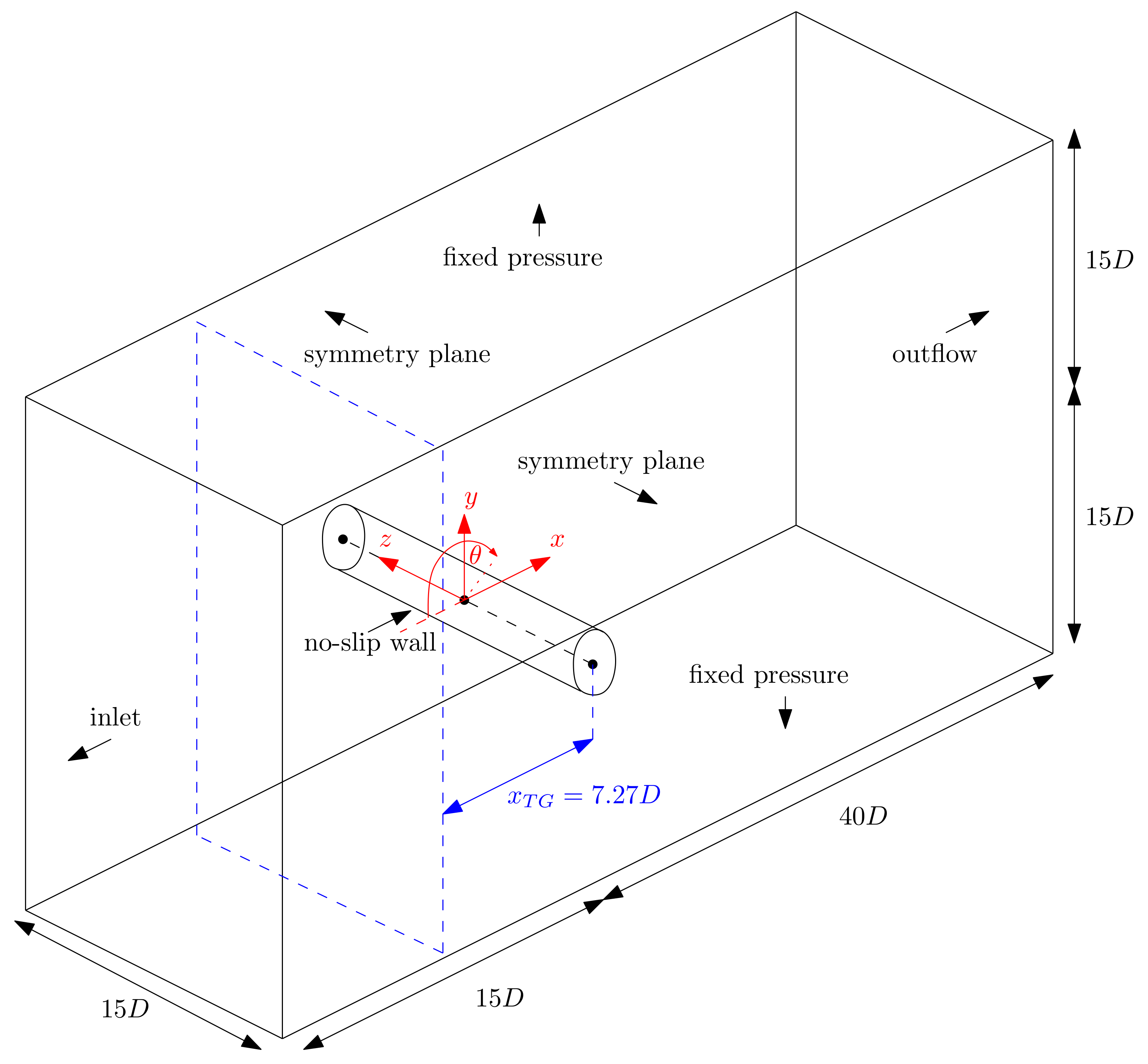
In order to generate a resolved, turbulent inflow, the synthetic approach described and implemented in [30] was used. This method is based on the work by [31,32], wherein random numbers are transformed into turbulent fluctuations correlated in space and time.
In this method, random numbers, r m , l , i , with a zero mean and unit variance, are generated on a 2D Cartesian grid at each time-step. The indices m , l indicate the position on the 2D grid, and i refers to the velocity component. These numbers are spatially correlated using assumed exponential correlation functions, and their temporal correlation with the numbers generated during the previous timestep is ensured using
Ψ i t = Ψ i t Δ t exp π Δ t 2 T + ψ i t 1 exp π Δ t 2 T .
Here, T = L / U i is the Lagrangian time-scale based on the desired integral length scale L . The spatially and temporally correlated numbers are transformed to velocity fluctuations using
U i = a i j · Ψ i ,
in which a i j indicates the Lund transformation matrix, which is based on a Cholesky decomposition of the desired Reynolds stress tensor τ i j . In the current work, the modifications described in [29] are employed. This means that the desired velocity fluctuations are transformed into a body force in the momentum equations, using
F b , i = U i , i n f l o w + U i U i ρ U i ¯ L t g b ,
where U i , i n f l o w is the mean velocity as defined at the generator plane, U i comes from Equation (10) and U i is the instantaneous velocity in a cell obtained from the solver at the current non-linear loop. L t g indicates the distance in the flow direction over which the body-force term is applied, and b (taken here as approximately 0.15) is an arbitrary multiplication factor used to increase the convergence of the velocity towards the desired fluctuations. In this manner, the velocity field can be made to include the desired fluctuations while remaining divergence-free. This reduces spurious pressure fluctuations from being introduced into the flow and avoids deterioration of the iterative convergence. The choice of the b tuning factor has been made based on running precursory simulations of an empty domain with the same grid topology, free-stream grid cell size and time-step. Choice of the distance over which the source term is applied is connected to the arbitrary tuning factor, as typically, the larger the thickness of the plane, the smaller the tuning factor needs to be in order to achieve the desired turbulence intensity. However, care must be taken to ensure that the thickness of the plane is smaller than the turbulence length scales that are being created. Usually a single layer of cells has been found to be sufficient in practical terms.
Figure 1 compares the iterative convergence for all inflow turbulence levels, including the case without inflow turbulence. Almost identical trends are observed irrespective of the prescribed inflow turbulence levels, indicating that the body force approach for introducing inflow turbulence has no adverse effects on convergence. This is critically important for acoustic predictions, which can be polluted by numerical noise. Additionally, the number of outer loops per time-step remains approximately the same, highlighting the low computational overhead of the synthetic inflow turbulence generator (ITG).

3. Test Case

3.1. Description

The present work considers the flow around a circular cylinder at a Reynolds number of R e = U D / ν = 14,700 and M a = U / c 0 = 0.029 , and replicates the measurement setup of Maryami et al. [12]. For the chosen experimental condition, a freestream turbulence intensity of 5.1% and an integral length scale of 0.0239 m (1.086 cylinder diameters) have been reported. This data set allows for comparisons of fluctuating surface pressures, for computations with and without inflow turbulence, to validate the synthetic turbulence generation part of the proposed numerical methodology.
This case is then used to explore the effect of a range of inlet turbulence levels beyond what was tested in the reference data set. Parameters used in order to set up the simulations are described in Table 1 and aim to mimic the wind tunnel set up as closely as possible.

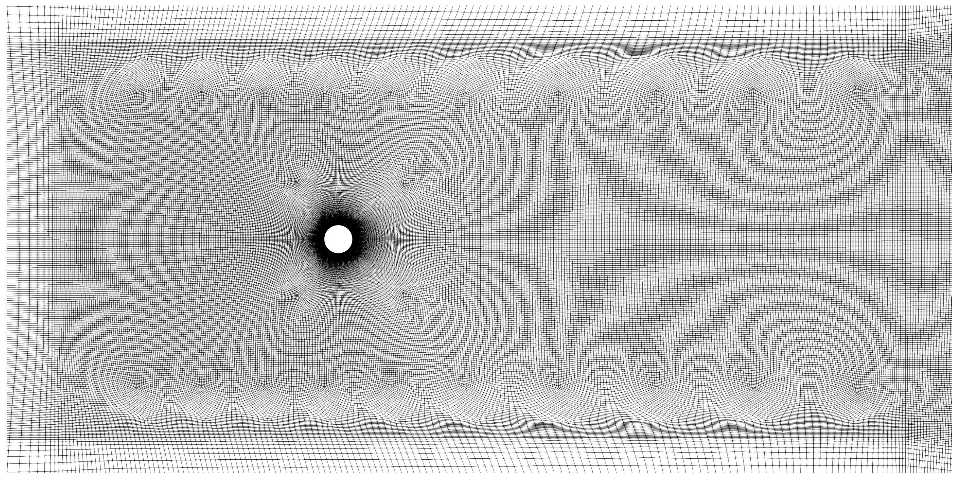
3.2. Domain and Grids

From the experimental data given by Norberg [33] and numerical results by Liefvendahl and Bensow [19], the spanwise correlation length for the considered Reynolds number is known to be between approximately four and five cylinder diameters. In the experiments of Maryami et al. [12], the cylinder span was 21 diameters, ensuring that the end effects play a minimum role on the flow. In the present simulations, S / D s i m = 15 was used as a compromise between computational cost and the desire to avoid a significant influence of the boundaries and boundary conditions on the spanwise correlation of the flow. The computational domain extends 15 D upstream, 40 D downstream, and ± 15 D in the cross-flow direction. An overview of the numerical domain, relative position of the ITG, boundary conditions and coordinate system is shown in Figure 2.
The grids were adapted from the one used by Pereira et al. [28], which had been optimised for quality and used for validation studies at low (3900) Pereira et al. [28] and high (140,000) Reynolds numbers [27]. As such, they were deemed a suitable starting point for the present work, which concerns a Reynolds number bound by those of the previous studies. An example visualisation of the grid is shown in Figure 3. At the chosen refinement level, 36.6 M cells were used. 230 cells were placed along the span and 925 around the circumference of the cylinder. A maximum wall-normal normalised first cell size y 1 + = y 1 u τ / ν below 1 was ensured for all cases, with a mean of approximately 0.3 . Here, u τ = τ w / ρ is the friction velocity, with τ w being the wall shear stress. In practice, cases without inflow turbulence required smaller cell sizes in order to meet this resolution criterion. Therefore, in order to employ the same grids for all conditions, y + values well below the threshold of 1 were reached for the cases with the inflow turbulence generator enabled. Maximum values in the streamwise ( x + ) and spanwise ( z + ) directions were below 15 and 150, respectively. This is slightly coarser than requirements for large eddy simulation (LES [34,35], but was considered acceptable, since f k = 0.25 implies that less turbulence is resolved than is typically recommended for LES (about 20%) [36]. Another important consideration related to PANS discussed by [16] is the aspect ratio of cells at the wall. For aspect ratios that are too high, turbulence at the wall may have a skewed energy content. This can adversely affect results, especially in terms of surface pressures. Currently, the maximum aspect ratio on the wall is equal to 120, slightly above the recommended value of 70. The present results did not indicate substantial issues related to this, but future studies should aim to achieve lower aspect ratio values.

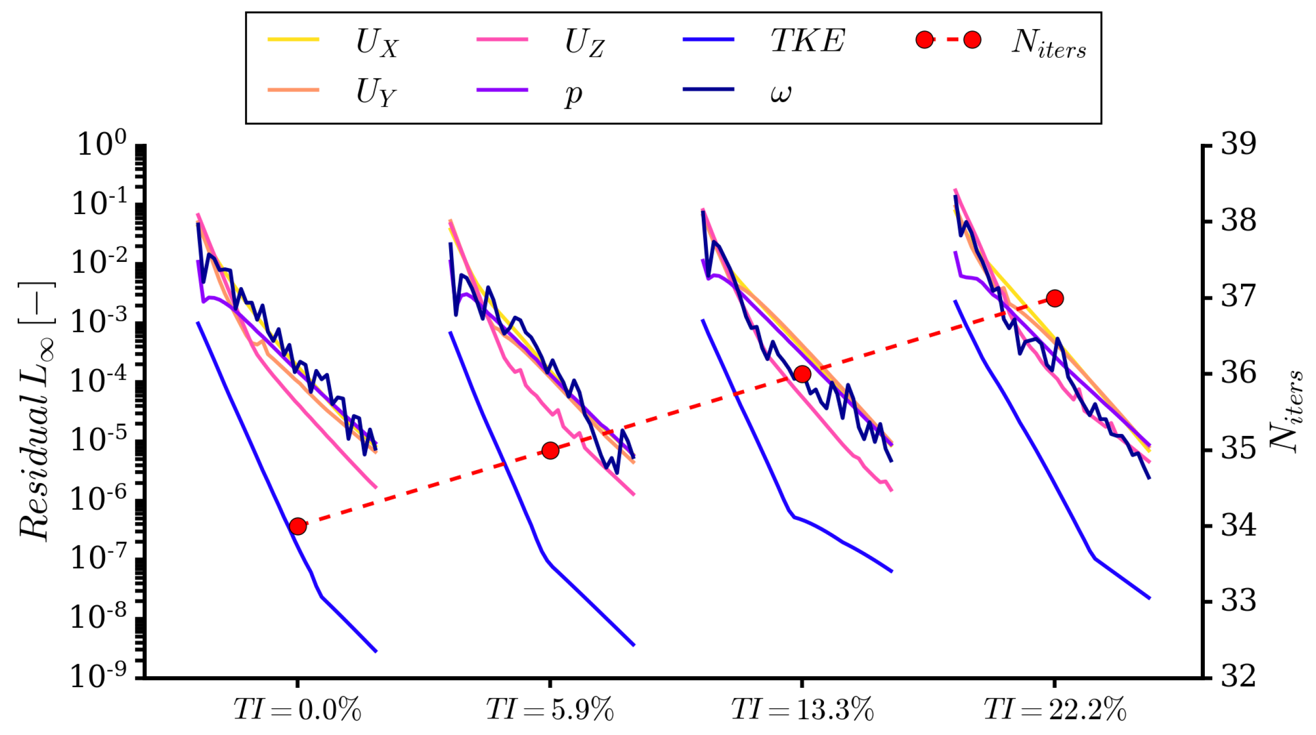
3.3. Numerical Setup

Simulations were run using a second-order time-implicit time integration with a fixed timestep size of Δ t = 1 × 10 5 s, or Δ t * = Δ t U / D = 4.5 × 10 3 , resulting in a maximum Courant number below 2. This was necessary to capture the dynamics of the unsteady flow around the cylinder and preliminary simulations with larger timesteps yielded unsatisfactory results. All of the simulations were run using 320 dual 2.0 GHz Intel Skylake processors. Typical wall clock times of around a week were necessary in order to obtain sufficiently long time traces for the case.
The QUICK discretisation scheme was used for the convective fluxes in the momentum and turbulence transport equations, following the work of [29]. This scheme aims to balance second-order accuracy with stability, a requirement necessary for the use of the proposed set up in practical situations. However, use of a central scheme with a small amount of upwinding might also be acceptable and needs to be investigated in the future. Diffusive terms were treated with a second-order central scheme. Approximately 30 outer loops using the SIMPLE algorithm were needed per timestep to achieve the desired L convergence criterion of 10 5 , where the residuals are normalised using the diagonal of the matrix on the left-hand side of the linear system of equations.
A Dirichlet velocity boundary condition was imposed at the inlet boundary. Fixed value of pressure was prescribed at the top and bottom sides of the domain (parallel to the cylinder axis). At the outflow, a Neumann velocity condition was imposed. In order to minimise the negative effects of strong vortices reflecting from the downstream boundary, substantial grid coarsening was employed in the wake in order to deliberately dissipate any remaining vortical structures. Spanwise boundaries normal to the cylinder axis were treated as symmetry planes. Consideration had been given to using cyclic boundaries in order to reduce the domain size and cost of the simulations, but it was decided to use a wider domain in order not to artificially affect the natural spanwise length scales occurring in the flow. A standard no-slip wall was employed at the cylinder surface.

3.4. Signal Processing

All of the presented results have been obtained from analysing 200 non-dimensional time units, defined as T = U / D , collected after the simulations had achieved fully developed flow. This corresponded to approximately 40 shedding cycles, with at least as many having been discarded in order to remove the effect of start-up transients from the analyses.
For spectral analysis, the signals were then processed using the Welch algorithm [37] with 50% overlap between each of the four segments into which the traces were subdivided. In order to smooth the frequency domain results, their narrowband forms were smoothed using a one-sixth octave bandwidth top hat filter. This involves defining frequency bands with centre frequencies f c separated by one-sixth of an octave ( 2 1 / 6 ), resulting in lower and upper limits of the bandwidth filter f l = 2 1 / 12 f c and f u = 2 1 / 12 f c , with 1 kHz used as the baseline centre frequency. The power spectral density (PSD) is integrated within each band, and subsequently corrected back to narrowband spectrum level, using
ϕ ^ ( f c ) = f l f u ϕ ( f ) d f Δ f ,
where Δ f = f u f l = ( 2 1 / 12 2 1 / 12 ) f c 0.1156 f c .

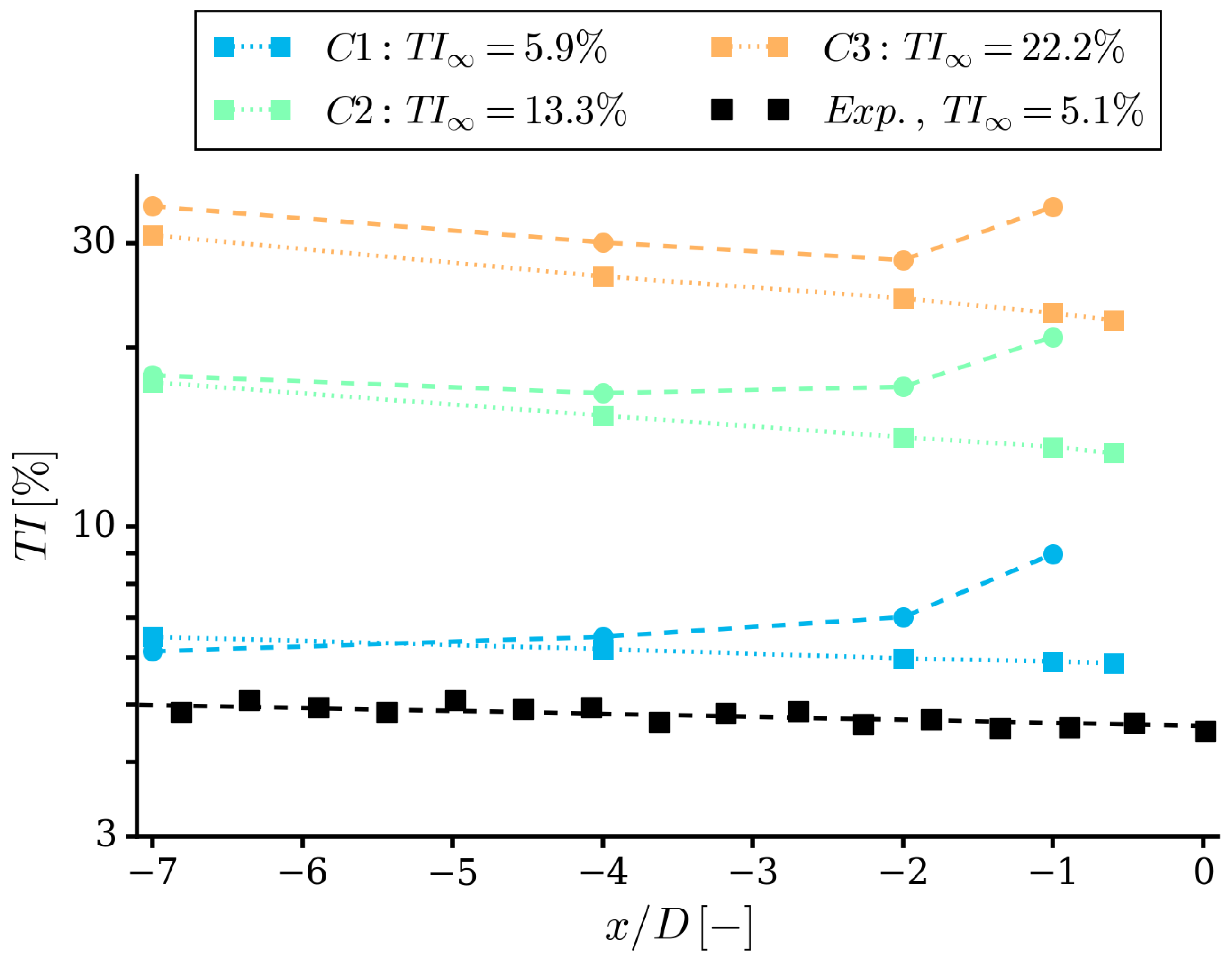
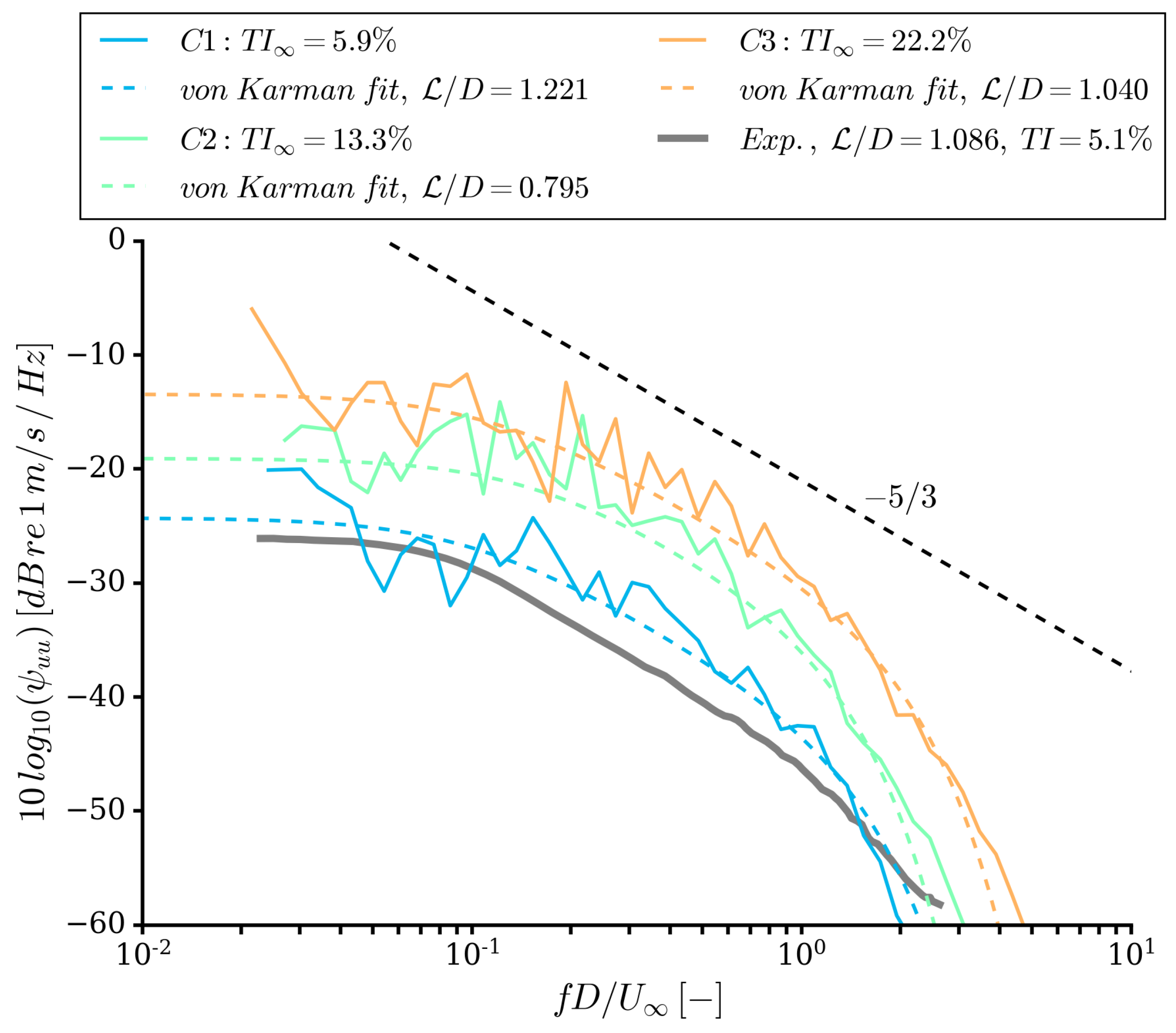
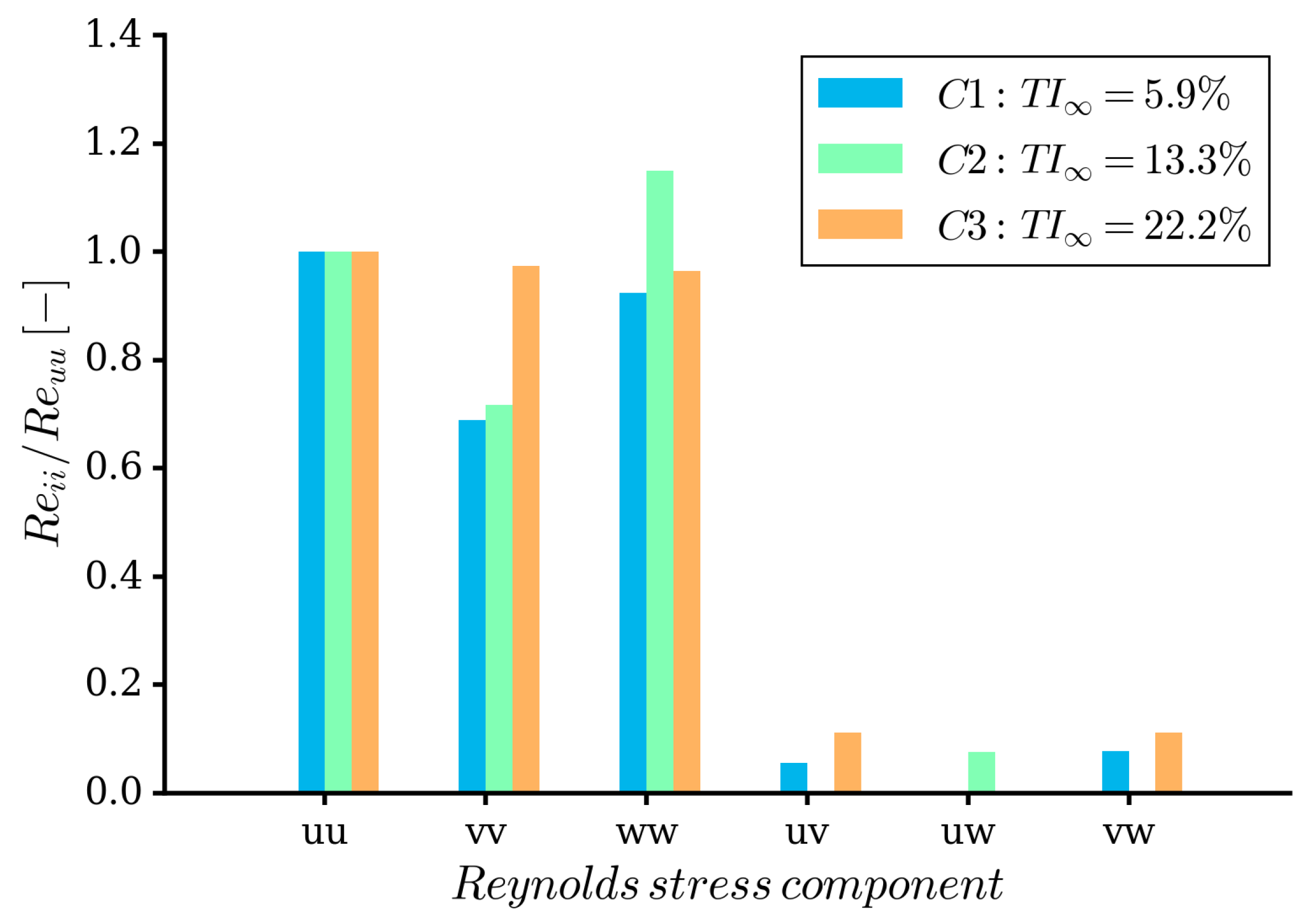
3.5. Inflow Turbulence Statistics

The turbulence intensities addressed in the present work cover a large range, up to values which are difficult to achieve experimentally for grid-generated turbulence without inducing anisotropy. However, high turbulence intensity values well in excess of 10% are encountered in ship wakes [38,39]. Being able to predict such challenging conditions is therefore of interest from the point of view of predicting broadband marine propeller noise, which is the long-term aim of the present work.
Since in the current implementation of the inflow turbulence generator, the desired velocity fluctuations are transformed to a momentum source using an arbitrary tuning factor (see Equation (11), replicating certain desired inflow turbulence properties requires a tuning procedure that comes at a high computational cost. This was carried out by first simulating the setup with only the inflow generator present in an empty domain of the same size and similar grid topology as that used for the cylinder simulations. The tuning coefficient was iteratively varied for each case until a desirable match was achieved. The same settings were then applied for the cylinder simulations. However, because of small differences in the exact grid size, timestep, and iterative convergence, the spectra obtained in the presented cases differed slightly from those in the initial tuning set.
In order to further examine the effect of grid resolution on the inflow velocity spectrum decay, the cell size upstream of the cylinder was also varied during the tuning of the inflow turbulence generator. It was found that it was necessary to maintain a resolution of at least 10 cells per integral length scale. When this condition was not met, the spectra remained within several dB from the median up to S t = f D / U 0.65 . For higher frequencies, an influence of the diminishing increasing filter width was seen in the decaying part of the spectrum. Beyond S t = 2.2 , all spectra had decayed to such an extent that the differences due to cell size became indistinguishable.
Cases with an empty domain were also used to assess the level of turbulence dissipation between the ITG and the cylinder. The ITG was located 7.27 D upstream of the cylinder axis, which corresponded to one of the locations of the turbulence generating grid in the experiments. In the present case, using much longer development lengths, as seen in some of the experimental conditions, was not necessary since the characteristics of inflow turbulence could be adjusted to match the desired values without relying on natural decay downstream of a turbulence-generating wire grid. The prescribed turbulence integral length scale was set to the measured value, and three different turbulence intensities were used in addition to the reference case, for which a uniform, steady inflow was applied, corresponding to the wind tunnel without grid.
For all the simulated cylinder cases, inflow turbulence properties were monitored at several locations upstream of the cylinder, both at the centreline ( y / D = 0 ) and above the cylinder ( y / D = + 4.5 ), as seen in Figure 4. It is observed that the turbulence intensity on the centreline in the vicinity of the cylinder increases, while above the cylinder it continues to decay. This effect is expected due to the distortion and blockage effects caused by the cylinder [14], as well as by the fact that the local flow velocity reduces when approaching the cylinder. Therefore, spectra and Reynolds stresses were monitored directly above the cylinder ( x / D = 0 , y / D = + 4.5 ) to be compared with measurements.
Figure 5 presents the inflow velocity spectrum computed for all cases, also showing data measured by Maryami et al. [12]. The frequency axis has been normalised to give the Strouhal number. The turbulence intensity found in the simulation is larger than the experimental value. It can be seen that in the low- and medium-frequency range, the agreement between the simulation and experiments is close, within several dB. The numerically predicted spectral levels are higher, which is consistent with the over-prediction of the inflow turbulence intensity by 0.8%. Assuming a quadratic dependency of noise on the turbulence intensity [40], a relative difference in TI between the cases of 15% results in an effect of around 1.3 dB, which for the current studies is considered acceptable. Both spectra exhibit the expected −5/3 decay slope. At high frequencies—taken as about S t > 1.5 —the computed spectrum begins to fall off due to the cut-off caused by the computational grid, resulting in lower spectral levels than the experimental data.
Reynolds stresses have also been computed in order to evaluate the isotropy properties of the turbulence generator. Figure 6 demonstrates that this has been achieved to a satisfactory degree, since the normal components are all close to equal, while the shear components are negligible, thereby confirming that the inflow turbulence is close to isotropic.
The computed integral length scales were extracted by fitting von Kármán spectra to the power spectral density functions of the computed velocity (as shown in Figure 5). The resulting values for all cases are presented in Table 2.
It is noted that both the turbulence intensity and length scale for case C1 are over-predicted, even after several tuning simulations. This illustrates a potential shortcoming of the tuning procedure for the current version of the inflow turbulence generator, where both the tuning coefficient and the data fitting approach influence the results.
The predicted dominant turbulence frequency may be defined as f L = U / L , and varies between approximately 375 and 575 Hz for the investigated test cases. This corresponds to Strouhal numbers between about 0.80 and 1.25. While these frequencies are above the main vortex shedding frequency of the cylinder, which occurs at a Strouhal number of about 0.2, interaction between the inflow turbulence and cylinder flow can still be expected, since there is a high level of turbulence kinetic energy at low frequencies.

4. Results

In the results, the integral quantities and flow field are firstly investigated and compared against experimental results. Secondly, the effect of inflow turbulence on the mean and fluctuating surface pressure is examined, since these results are directly associated with the noise sources of interest.

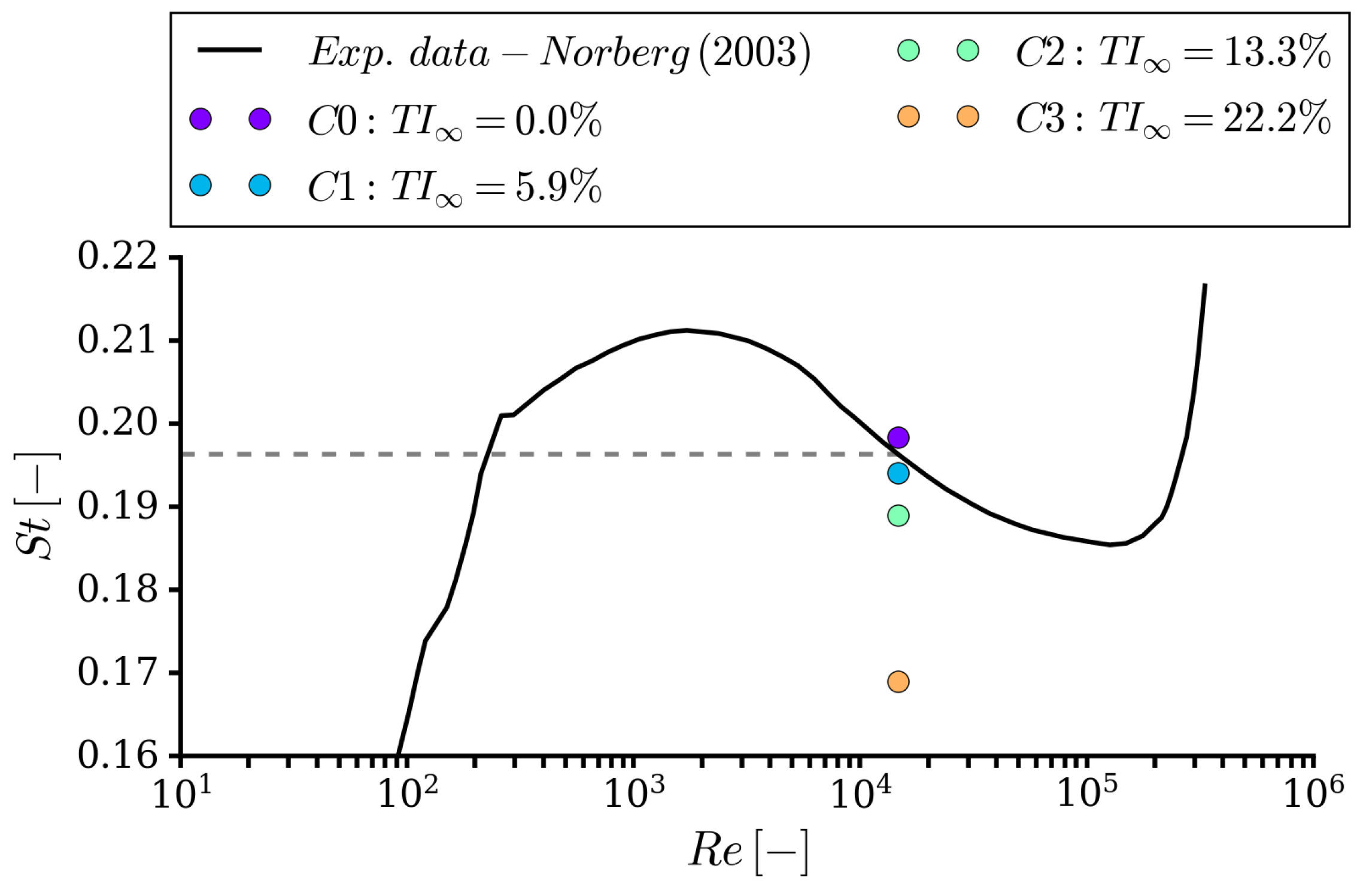
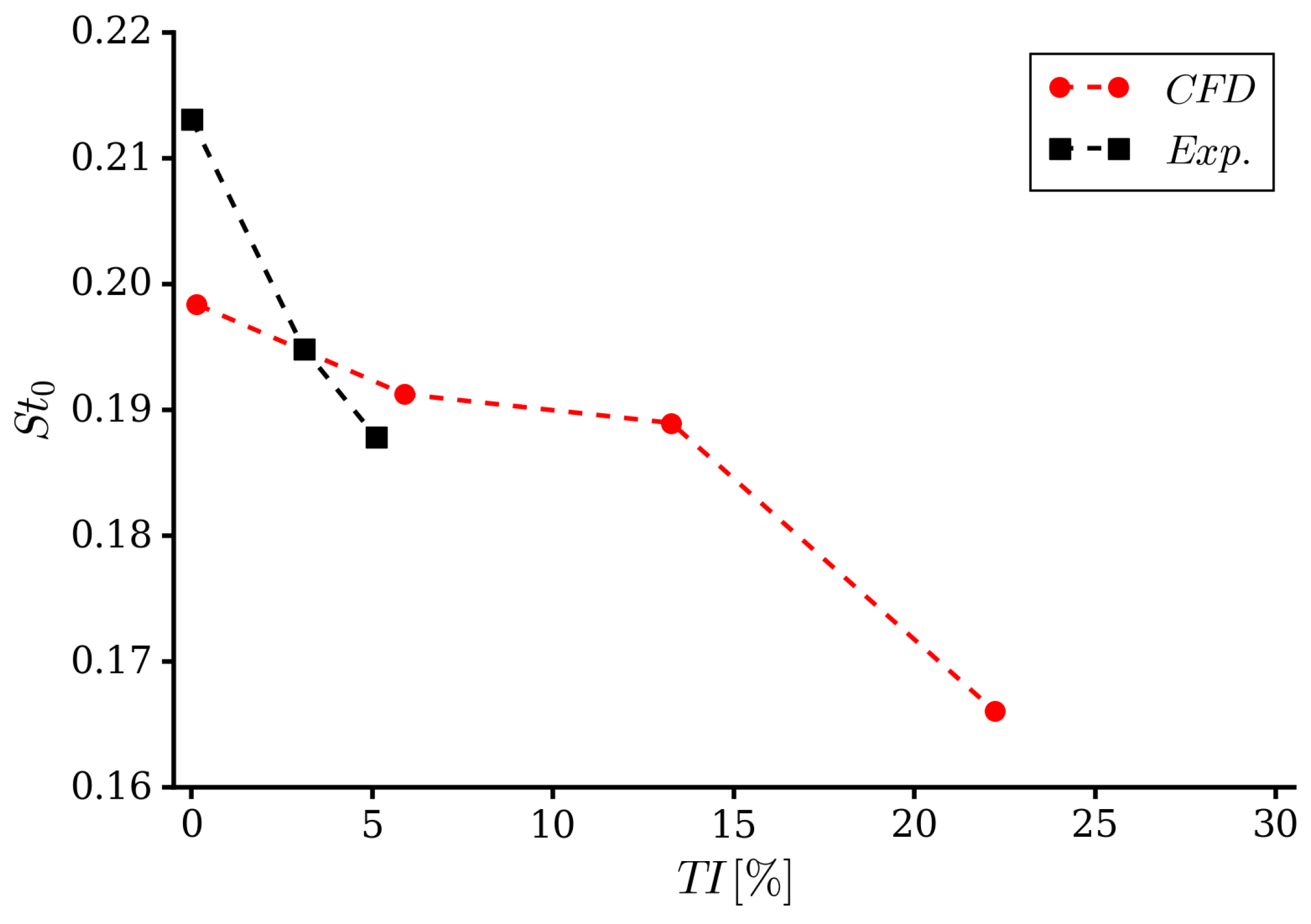
4.1. Integral Quantities and Flow Field

Figure 7 presents the computed mean drag coefficient C D = F · e x ¯ / S D q , where F is the force vector, e x the unit vector in the axial direction, and q = 1 2 ρ U 2 the reference dynamic pressure. Numerical results for all values of inflow turbulence intensity are compared to results from the literature. It is observed that the average force value is well-captured, with the relative error for the case with no inflow turbulence equal to 0.6% of the experimental value. For all the other cases, the effect of inflow turbulence on the drag is minimal. This is unsurprising, as isotropic turbulence should induce velocity fluctuations in all directions, which are expected to yield a net zero change in local incidence angle and velocity magnitude.
The frequency content of the lift coefficient C L = F · e y ¯ / S D q is given in Figure 8 as a function of inflow turbulence intensity level. With increasing turbulence intensity, the broadband level of the spectrum rises, consistent with a higher level of force oscillations induced by the incident turbulent flow. The peak of the lift coefficient spectrum also becomes wider and shifts slightly to lower frequencies with more turbulence.
The lift spectrum was also used to estimate the shift in the Strouhal number at the primary vortex shedding frequency resulting from increased inflow turbulence levels. The results are depicted in Figure 9. For the simulation without inflow turbulence, excellent agreement with the experiments may be seen. An increase in T I leads to a decrease of S t , which suggests that the freestream eddies interfere with the growth of the shear layer and accelerate the shedding of vortices. This observation can be likened to the effect of increasing Reynolds numbers on shedding behaviour, as demonstrated by the experimental data in Figure 9, and reported by Norberg and Sunden [41] for cases with and without inflow turbulence. A similar trend was also observed by [12], as seen in Figure 10.
The interaction of the vortical wake generated by the cylinder with inflow turbulence of increasing intensity is examined in Figure 11. At intermediate levels, when the strength of the von Kármán vortices is larger than those generated upstream, one may still distinguish a clear shear layer and pockets of shed vorticity, though these are disturbed by the freestream turbulent flow and dissipate more quickly. At vorticity levels approaching those generated by the cylinder itself, a different picture appears. The von Kármán vortices can still be observed, due to their larger size. However, downstream of the cylinder, the von Kármán vortices tend to break up into smaller structures under the influence of the inflow turbulence.
The mean axial velocity in the cylinder wake is depicted in Figure 12 at a streamwise position where the source experimental results by Maryami et al. [12] reported the largest influence of inlet turbulence. For all the conditions, the profiles outside of the wake of the cylinder appear similar. Directly downstream, however, cases with prescribed inflow turbulence show positive velocities at the centreline, with the minimum velocity at y / D = 0 increasing from 0.15 to ≈0.2. This indicates a shorter length of the separated flow region and is consistent with the trend observed in the experiments by Maryami et al. [12]. However, the computed velocities are substantially lower than those reported in the measurements. A similar trend is visible in Figure 13, which shows the mean axial velocity along a line directly behind the cylinder. Here, the computed velocity takes longer to recover to a near-constant level than in the measurements. On the other hand, the streamwise location at which recirculation disappears has been captured very well.
Root mean square (RMS) velocity fluctuations monitored in the wake are shown in Figure 14 and Figure 15. For the transverse cut, the velocity fluctuations at the centreline and in the shear layer are relatively unaffected by the inflow turbulence intensity, with only a modest reduction for the case without inflow turbulence. This trend is consistent with measurements by Maryami et al. [12], despite the apparent over-estimation of fluctuating velocities in the present study. A different trend is observed for the values computed at the centreline, which are compared to data from Norberg and Sunden [41]. Here, the current simulations under-predict the fluctuations directly behind the cylinder, that is, for x / D 2 . On the other hand, the curve without inflow turbulence does show the same characteristic two-peak shape in this region, and the fluctuations in the wake appear to be captured accurately. Another notable feature is the relative increase of turbulence levels in the direct wake of the cylinder with increasing inflow turbulence levels.
Figure 16 compares the velocity spectra at the wake centre line at two downstream positions. For condition C 0 , there is a clear peak in the spectra due to the wake flow. The difference in Strouhal number at which these peaks occur is due to the different downstream positions. At x / D = 0.5 , the peak occurs at f D / U = 0.2 , while further downstream, the peak switches to the second harmonic, at f D / U = 0.4 . The inclusion of inflow turbulence suppresses these peaks, which corresponds to the changes in the wake flow presented in Figure 11. Furthermore, the frequency at which the peak occurs at x / D = 0.5 may be seen to reduce as more TI is included, up until the point where the peak is no longer discernible for the case with highest inflow turbulence intensity.

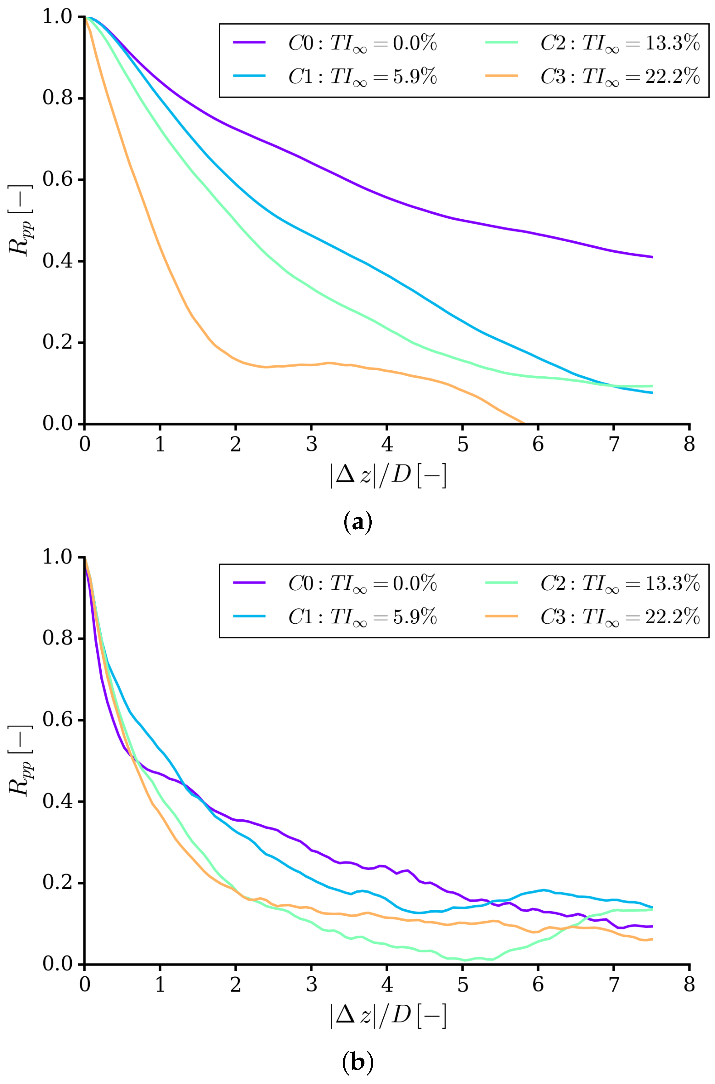
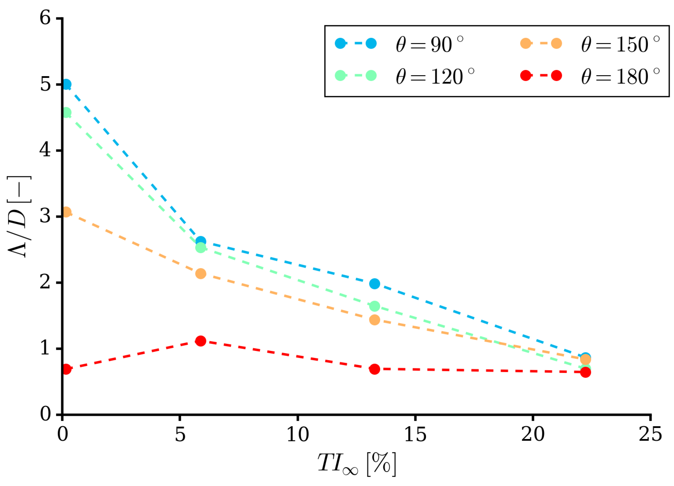
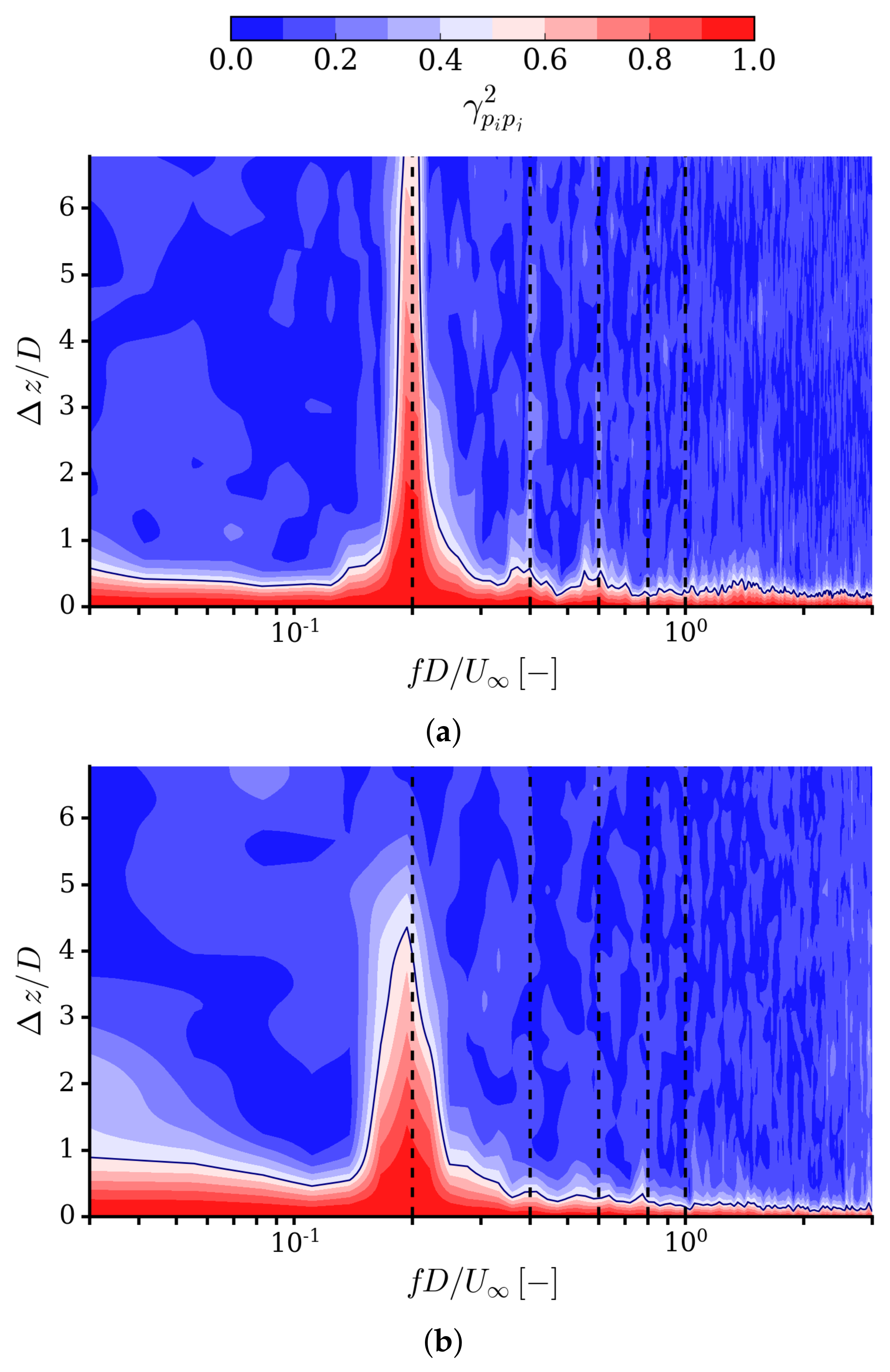
4.2. Surface Pressure

The average pressure coefficient C ¯ p = p ¯ / q around the mid-span of the cylinder is shown in Figure 17a. Two comparison data sets are presented, which enclose the current test case in terms of Reynolds number. A good qualitative agreement is found for results both with and without inflow turbulence, with the largest discrepancy observed at about θ = 90 , where the pressure is over-predicted for case C 0 . Notably, this discrepancy disappears with the addition of inflow turbulence. The circumferential distribution of the RMS surface pressure fluctuations C p = p 2 ¯ / q is given in Figure 17b for varying inflow turbulence intensities. For case C 0 , the peak values appear to be under-estimated by approximately 0.05, but the overall trend is captured well. Increasing the inflow turbulence intensity increases the fluctuations at all locations. The largest increase is in the upstream direction and is a direct consequence of turbulent flow interacting with the stagnation region of the cylinder. Case C 3 —with the highest inflow turbulence levels—is distinct from the others because the peak occurring at approximately 80 disappears, indicating large changes in the boundary layer separation and wake dynamics, as already identified in Figure 11. Although not directly comparable due to the different Reynolds numbers and turbulence intensities, the experimental data by [41] shown in the figure may be used for qualitative comparison with the trends seen in the present numerical results. It may be seen that in the measurements, increasing the Reynolds number leads to an increase in surface pressure fluctuations. A similar effect is observed when the amount of inflow turbulence is increased. Here, the angular position of the peak value remains constant but its magnitude is raised, as are the RMS values elsewhere around the cylinder. The same trends are observed in the presented simulation results up until very large freestream turbulence levels well in excess of 15%.
Figure 18 shows the normalised two-point spanwise pressure correlation R p p at two different angular positions. This is defined as
R p p ( θ , Δ z ) = p ( θ , t ) p ( θ , Δ z , t + τ ) ¯ p 2 ( θ , t ) ¯ ,
where Δ z is the spanwise probe separation, and τ , the time lag. The correlations are taken relative to the domain centreline, and averaged over the positive and negative spanwise directions, as well as the top and bottom sides of the cylinder where possible.
The differences in spanwise correlation between the four cases is most pronounced at the top of the cylinder, where the higher correlation level over the entire span for case C 0 indicates the dominance of large two-dimensional shed vortices. With the addition of more and more inflow turbulence, the correlation steadily decreases at this location due to the interaction of these vortices with the freestream eddies. On the leeward side, on the other hand, the different cases show a more similar behaviour because the flow here is always in a turbulent state, independent of the inflow turbulence levels.
These results may also be used in order to compute the spanwise correlation length as
Λ ( θ ) = lim L z 0 L z R p p ( θ ) d Δ z .
This is presented in Figure 19 for all angular positions for which data were sampled in the simulations. It can be seen that even a relatively small amount of inflow turbulence has a profound effect on the spanwise correlation of the flow, which becomes progressively smaller the more turbulence is added. This may be explained by the inflow turbulence becoming the dominant source of velocity fluctuations the higher the TI. These break up the spanwise flow structures that would be present in the undisturbed flow. In the case of the wake of the cylinder, the turbulent scales are small to begin with, and hence, the addition of inlet turbulence has little effect on the predicted length scales.
More insight into the changes in the flow induced by the inflow turbulence can be obtained using frequency-domain analyses of the surface pressures. Here, point power spectral densities ϕ p for six azimuthal positions are depicted in Figure 20, and squared spanwise coherence γ 2 at θ = 90 for conditions C 0 and C 1 , in Figure 21. This second quantity is defined as
γ 2 ( f , θ , Δ z ) = | ϕ p p ( f , θ , Δ z ) | 2 ϕ p p 2 ( f , θ ) ,
with ϕ p p the cross-power spectral density:
ϕ p p ( f , θ , Δ z ) = 1 2 π r p p ( θ , Δ z ) e i ω τ d τ ,
where
r p p ( θ , Δ z ) = p ( θ , t ) p ( θ , Δ z , t + τ ) ¯
is the two-point spanwise correlation. The PSD is recovered from Equation (16) for Δ z = 0 .
The results in Figure 20 are also compared to the measured data from Maryami et al. [12] for conditions C 0 and C 1 . At the stagnation point of the cylinder, the spectra without inflow turbulence show large differences (>10 dB) from measured values, although the levels are much lower than for the other cases, and should be considered negligible (see Figure 17). Values computed with inflow turbulence match the experimental measurements more closely, although worse agreement is observed at higher frequencies due to the numerical cut-off frequency of the inflow turbulence (Figure 5).
Moving towards the back of the cylinder, all the spectra computed without inflow turbulence match the experiments quite closely, with similar peak levels and overall features. In contrast, the spectrum computed with inflow turbulence, shows bigger discrepancies than on the forward-facing part of the body. At θ = 180 , the simulated spectrum resembles the spectrum obtained with a uniform inflow more than the experimentally measured spectrum. Despite this, cases with higher prescribed turbulence values follow the same general trend as what was observed experimentally, namely, a significant increase in broadband levels. Part of the explanation is that—even though the computed turbulence intensity is somewhat higher than the measured value—the distribution of fluctuations across the frequency range is not identical. There is less energy content at the middle and higher frequencies. This translates into a different cascade of turbulent scales in the freestream, which then manifests itself in the surface pressure spectra. Where the flow physics are more straightforward on the upstream part of the body, the agreement between computations and measurements remains satisfactory. However, further downstream the freestream turbulence needs to interact with the shear layer and fluctuations in the wake of the cylinder in a realistic manner. If the distribution of scales is not predicted correctly, these physical phenomena can be incorrectly represented in the simulations. The reason for this is most likely numerical dissipation. While the used grids are fine enough in order to represent the freestream turbulence and the flow around the cylinder without inflow turbulence, the grid may still be filtering out some of the smaller scales. This has little effect on the two flows independently, but could affect their interaction.
For both conditions, the shedding frequency is clearly visible due to the high spanwise coherence, although for C 1 , the coherence decays faster as a function of position (in agreement with the spanwise correlation), and exhibits a wider peak, which is shifted towards the lower frequencies (as also found for the lift spectra). For case C O , there is also a higher coherence at the second and third harmonics of the vortex shedding frequency. This behaviour is suppressed by inflow turbulence.

5. Conclusions

The interaction between a circular cylinder and freestream turbulence was simulated using PANS with a synthetic ITG. The hydrodynamic results are compared to experimental results for the test case, as well as other data for similar conditions available from the literature.
The use of the ITG with momentum sources is a computationally efficient method to generate resolved inflow turbulence without adversely affecting solution convergence, making this method very well-suited to applications involving acoustics. One of the downsides of the current method is the required tuning of the ITG settings when replicating particular experimental conditions. This could potentially be improved by modifying the equation employed to transform the velocity fluctuations to momentum sources.
Results which could be compared to measurement data—both with (C1) and without (C0) inflow turbulence—have good agreement in terms of mean surface pressure and wake velocity. The surface pressure spectra show deviations from the measurement data of only a few decibels across much of the frequency range. Larger discrepancies were found at high frequencies (above 5–10 S t , depending on circumferential position), which are not well-resolved by the simulations. Cases with higher turbulence intensities, for which no validation material is available, exhibit large differences in terms of the fluctuating quantities, compared to the validated cases.
In the flow without inflow turbulence, there is a high spanwise correlation before the shear layer starts to transition to turbulence beyond θ = 90 . When using the ITG, the baseline flow characterised by von Kármán shedding remains visible in the wake visualisations. However, in the frequency spectra, the peak due to vortex shedding becomes less pronounced, with an associated reduction in spanwise correlations, while the broadband level becomes higher with increasing inflow turbulence intensity.
As part of future work, we intend to extend the validation exercise to farfield radiated noise. These predictions can be made by post-processing the hydrodynamic flow solution using the Ffowcs Williams–Hawkings acoustic analogy [44].

Author Contributions

Conceptualisation, A.K.L.; methodology, A.K.L. and M.K.; investigation, A.K.L.; writing—original draft preparation, A.K.L., M.K. and T.L.; writing—review and editing, A.K.L., M.K. and T.L.; visualisation, A.K.L. All authors have read and agreed to the published version of the manuscript.

Funding

Parts of this work were carried out on the Iridis5 (University of Southampton) cluster. The research was partly supported financially by the Dutch Research Council (NWO), as part of the NOISOURCE project (ALWTW.2016.008).

Conflicts of Interest

The authors declare no conflict of interest. The funders had no role in the design of the study; in the collection, analyses, or interpretation of data; in the writing of the manuscript, or in the decision to publish the results.

References

  1. Churchfield, M.J.; Lee, S.; Michalakes, J.; Moriarty, P.J. A numerical study of the effects of atmospheric and wake turbulence on wind turbine dynamics. J. Turbul. 2012, 13, N14. [Google Scholar] [CrossRef]
  2. Milne, I.A.; Graham, J.M. Turbulence velocity spectra and intensities in the inflow of a turbine rotor. J. Fluid Mech. 2019, 870, 870R31–870R311. [Google Scholar] [CrossRef]
  3. Kornev, N.V.; Taranov, A.; Shchukin, E.; Kleinsorge, L. Development of hybrid URANS-LES methods for flow simulation in the ship stern area. Ocean. Eng. 2011, 38, 1831–1838. [Google Scholar] [CrossRef]
  4. Liefvendahl, M.; Troëng, C. Simulation based analysis of the hydrodynamics and load fluctuations of a submarine propeller behind a fully appended submarine hull. In Proceedings of the 29th Symposium on Naval Hydrodynamics, Gothenburg, Sweden, 26–31 August 2012. [Google Scholar]
  5. Tian, Y.; Cotté, B. Wind turbine noise modeling based on Amiet’s theory: Effects of wind shear and atmospheric turbulence. Acta Acust. United Acust. 2016, 102, 626–639. [Google Scholar] [CrossRef] [Green Version]
  6. Zanon, A.; De Gennaro, M.; Kuehnelt, H.; Giannattasio, P. Assessment of the broadband noise from an unducted axial fan including the effect of the inflow turbulence. J. Sound Vib. 2018, 429, 18–33. [Google Scholar] [CrossRef]
  7. Hutcheson, F.; Brooks, T. Noise radiation from single and multiple rod configurations. Int. J. Aeroacoustics 2012, 11, 291–334. [Google Scholar] [CrossRef] [Green Version]
  8. Amiet, R.K. Acoustic radiation from an airfoil in a turbulent stream. J. Sound Vib. 1975, 41, 407–420. [Google Scholar] [CrossRef]
  9. Zamponi, R.; Satcunanathan, S.; Moreau, S.; Ragni, D.; Meinke, M.; Schröder, W.; Schram, C. On the role of turbulence distortion on leading-edge noise reduction by means of porosity. J. Sound Vib. 2020, 485, 1–22. [Google Scholar] [CrossRef]
  10. Bilka, M.; Kerrian, P.; Ross, M.; Morris, S. Radiated sound from a circular cylinder in a turbulent shear layer. Int. J. Aeroacoustics 2014, 13, 511–532. [Google Scholar] [CrossRef]
  11. Maryami, R.; Ali, S.A.S.; Azarpeyvand, M.; Afshari, A.; Dehghan, A.A. Turbulent flow interaction with a circular cylinder. In Proceedings of the 25th AIAA/CEAS Aeroacoustics Conference, Delt, Netherlands, 20–23 May 2019; pp. 1–14. [Google Scholar]
  12. Maryami, R.; Showkat Ali, S.A.; Azarpeyvand, M.; Afshari, A. Turbulent flow interaction with a circular cylinder. Phys. Fluids 2020, 32, 015105. [Google Scholar] [CrossRef] [Green Version]
  13. Liefvendahl, M.; Bensow, R.E. Simulation-based investigation of foil-turbulence interaction noise. In Proceedings of the 33rd Symposium on Naval Hydrodynamics, Osaka, Japan, 31 May–5 June 2020. [Google Scholar]
  14. Britter, R.E.; Hunt, J.C.; Mumford, J.C. The distortion of turbulence by a circular cylinder. J. Fluid Mech. 1979, 92, 269–301. [Google Scholar] [CrossRef]
  15. Li, S.; Rival, D.E.; Wu, X. Sound source and pseudo-sound in the near field of a circular cylinder in subsonic conditions. J. Fluid Mech. 2021, 919, 1–33. [Google Scholar] [CrossRef]
  16. Pereira, F.S.; Eça, L.; Vaz, G.; Girimaji, S.S. Toward Predictive RANS and SRS Computations of Turbulent External Flows of Practical Interest. Arch. Comput. Methods Eng. 2021, 28, 3953–4029. [Google Scholar] [CrossRef]
  17. Tutar, M.; Celik, I.; Yavuz, I. Modeling of effect of inflow turbulence data on large eddy simulation of circular cylinder flows. J. Fluids Eng. 2007, 129, 780–790. [Google Scholar] [CrossRef]
  18. Bulut, S.; Ergin, S. Effects of temperature, salinity, and fluid type on acoustic characteristics of turbulent flow around circular cylinder. J. Mar. Sci. Appl. 2021, 20, 213–218. [Google Scholar] [CrossRef]
  19. Liefvendahl, M.; Bensow, R.E. Simulation-based analysis of flow-generated noise from cylinders with different cross-sections. In Proceedings of the 32nd Symposium on Naval Hydrodynamics, Hamburg, Germany, 5–10 August 2018. [Google Scholar]
  20. Vaz, G.; Jaouen, F.; Hoekstra, M. Free-surface viscous flow computations: Validation of URANS code FRESCO. In Proceedings of the 28th International Conference on Ocean, Offshore and Arctic Engineering, Honolulu, HI, USA, 31 May–5 June 2009; American Society of Mechanical Engineers: New York, NY, USA, 2009; pp. 425–437. [Google Scholar]
  21. Girimaji, S.; Abdol-Hamid, K. Partially averaged Navier-Stokes model for turbulence: Implementation and validation. In Proceedings of the 43rd AIAA Aerospace Sciences Meeting and Exhibit, Reno, NV, USA, 10–13 January 2005. [Google Scholar]
  22. Germano, M. Turbulence: The filtering approach. J. Fluid Mech. 1992, 238, 325–336. [Google Scholar] [CrossRef]
  23. Pereira, F.; Vaz, G.; Eça, L.; Girimaji, S. Simulation of the flow around a circular cylinder at Re = 3900 with partially-averaged Navier-Stokes equations. Int. J. Heat Fluid Flow 2018, 69, 234–246. [Google Scholar] [CrossRef]
  24. Menter, F.; Kuntz, M.; Langtry, R. Ten years of industrial experience with the SST turbulence model. Turbul. Heat Mass Transf. 2003, 4, 625–632. [Google Scholar]
  25. Klapwijk, M.; Lloyd, T.; Vaz, G. On the accuracy of partially averaged Navier-Stokes resolution estimates. Int. J. Heat Fluid Flow 2019, 80, 108484. [Google Scholar] [CrossRef]
  26. Klapwijk, M.; Lloyd, T.; Vaz, G.; Van Terwisga, T. PANS simulations: Low versus high Reynolds number approach. In Proceedings of the VIII International Conference on Computational Methods in Marine Engineering (MARINE 2019), Gothenborg, Sweden, 13–15 May 2019; pp. 48–59. [Google Scholar]
  27. Pereira, F.; Eça, L.; Vaz, G.; Girimaji, S. On the simulation of the flow around a circular cylinder at Re=140,000. Int. J. Heat Fluid Flow 2019, 76, 40–56. [Google Scholar] [CrossRef]
  28. Pereira, F.S.; Eca, L.; Vaz, G.; Girimaji, S.S. Challenges in Scale-Resolving Simulations of turbulent wake flows with coherent structures. J. Comput. Phys. 2018, 363, 98–115. [Google Scholar] [CrossRef]
  29. Klapwijk, M.; Lloyd, T.; Vaz, G.; Van Terwisga, T. On the use of synthetic inflow turbulence for scale-resolving simulations of wetted and cavitating flows. Ocean. Eng. 2021, 228, 108860. [Google Scholar] [CrossRef]
  30. Klapwijk, M.; Lloyd, T.; Vaz, G.; Van Terwisga, T. Evaluation of scale-resolving simulations for a turbulent channel flow. Comput. Fluids 2020, 209, 104636. [Google Scholar] [CrossRef]
  31. Xie, Z.T.; Castro, I. Efficient generation of inflow conditions for large eddy simulation of street-scale flows. Flow Turbul. Combust. 2008, 81, 449–470. [Google Scholar] [CrossRef] [Green Version]
  32. Kim, Y.; Castro, I.; Xie, Z. Divergence-free turbulence inflow conditions for large-eddy simulations with incompressible flow solvers. Comput. Fluids 2013, 84, 56–68. [Google Scholar] [CrossRef] [Green Version]
  33. Norberg, C. Fluctuating lift on a circular cylinder: Review and new measurements. J. Fluids Struct. 2003, 17, 57–96. [Google Scholar] [CrossRef]
  34. Piomelli, U.; Balaras, E. Wall-layer models for large-eddy simulations. Annu. Rev. Fluid Mech. 2002, 34, 349–374. [Google Scholar] [CrossRef] [Green Version]
  35. Georgiadis, N.; Rizzetta, D.; Fureby, C. Large-eddy simulation: Current capabilities, recommended practices, and future research. AIAA J. 2010, 48, 1772–1784. [Google Scholar] [CrossRef]
  36. Pope, S.B. Turbulent Flows; Cambridge University Press: Cambridge, UK, 2000. [Google Scholar]
  37. Welch, P. The use of fast Fourier transform for the estimation of power spectra. IEEE Trans. Audio Electroacoust. 1967, 15, 70–73. [Google Scholar] [CrossRef] [Green Version]
  38. Lee, J.Y.; Paik, B.G.; Lee, S.J. PIV measurements of hull wake behind a container ship model with varying loading condition. Ocean. Eng. 2009, 36, 377–385. [Google Scholar] [CrossRef]
  39. Guilmineau, E.; Deng, G.B.; Queutey, P.; Visonneau, M.; Wackers, J. Detached Eddy Simulations of the Flow Around the Japan Bulk Carrier (JBC); Direct and Large-Eddy Simulation XI; Salvetti, M.V., Armenio, V., Fröhlich, J., Geurts, B.J., Kuerten, H., Eds.; Springer International Publishing: Cham, Switzerland, 2019; pp. 579–585. [Google Scholar]
  40. Blake, W.K. Mechanics of Flow-Induced Sound and Vibration, Volume 2. Complex Flow-Structure Interactions, 2nd ed.; Academic Press: London, UK, 2017. [Google Scholar]
  41. Norberg, C.; Sunden, B. Turbulence and reynolds number effects on the flow and fluid forces on a single cylinder in cross flow. J. Fluids Struct. 1987, 1, 337–357. [Google Scholar] [CrossRef]
  42. Norberg, C. Effects of Reynolds Number and a Low-Intensity Freestream Turbulence on the Flow around a Circular Cylinder. Ph.D. Thesis, Chalmers University, Gothenborg, Sweden, 1987. [Google Scholar]
  43. Lim, H.C.; Lee, S.J. Flow control of circular cylinders with longitudinal grooved surfaces. AIAA J. 2002, 40, 2027–2036. [Google Scholar] [CrossRef]
  44. Ffowcs Williams, J.E.; Hawkings, D.L. Sound generation by turbulence and surfaces in arbitrary motion. Philos. Trans. R. Soc. Math. Phys. Eng. Sci. 1969, 264, 321–342. [Google Scholar] [CrossRef]
Figure 1. L norm of the residuals and number of outer loops for a single timestep. Results from three simulations with increasing inflow turbulence levels and a reference simulation without resolved inflow turbulence. The residuals are normalised using the diagonal of the matrix on the left-hand side of the linear system of equations. A convergence tolerance of 10 5 was used, with the outer loop terminated once this level of convergence was reached.
Jmse 09 01274 g001
Figure 2. Schematic of the domain, including dimensions, boundary conditions, and coordinate system definition.
Jmse 09 01274 g002
Figure 3. Rendering of the structured grid topology for a coarse refinement level (5 M cells), showing cell sizes at a midspan cut through the domain.
Jmse 09 01274 g003
Figure 4. Inflow turbulence intensity levels monitored upstream of the cylinder, where the distance is given relative to the location of the cylinder. The final probe in the numerical results is located 0.1 D upstream of the cylinder. Circular and square data points indicate probes on the domain midplane ( y / D = 0 ) and a parallel plane ( y / D = + 4.5 ), respectively. Measurement values reported by [12] also shown for comparison.
Jmse 09 01274 g004
Figure 5. Inflow turbulence velocity power spectral densities at the axial location of the cylinder ( x / D = 0 ), for the cases studied numerically. Case C 1 is compared to the data reported by Maryami et al. [12].
Jmse 09 01274 g005
Figure 6. Reynolds stresses R e i i = u i u i ¯ sampled at x / D = 0 , normalised by the R e u u component.
Jmse 09 01274 g006
Figure 7. Mean drag coefficient for all cases (coloured markers) and experiments from various sources (grey markers) summarised by Norberg and Sunden [41].
Jmse 09 01274 g007
Figure 8. Power spectral density of lift coefficient. (a) Narrowband spectra, zoomed in on vortex shedding peak; (b) One-sixth octave filtered spectra.
Jmse 09 01274 g008
Figure 9. Predicted Strouhal number, computed from the lift power spectral density, compared to experimental values given by Norberg [33].
Jmse 09 01274 g009
Figure 10. Dominant Strouhal number extracted from lift coefficient spectra compared with data from [12].
Jmse 09 01274 g010
Figure 11. Distribution of instantaneous spanwise vorticity ω z * = ω z D / U . (a) [ T I = 0.0 % ]; (b) [ T I = 5.9 % ]; (c) [ T I = 13.3 % ]; (d) [ T I = 22.2 % ].
Jmse 09 01274 g011
Figure 12. Mean axial velocity, u ¯ / U , in the cylinder wake at x / D = 1.5 . Measurements from [12].
Jmse 09 01274 g012
Figure 13. Mean velocity, u ¯ / U , in the cylinder wake at y / D = 0 . Measurement data from [41].
Jmse 09 01274 g013
Figure 14. Root mean square axial velocity fluctuations, u / U , in the cylinder wake at x / D = 1.5 . Measurement data from [12].
Jmse 09 01274 g014
Figure 15. Root mean square axial velocity fluctuations, u / U , in the cylinder wake at y / D = 0 . Measurement data from [41].
Jmse 09 01274 g015
Figure 16. Velocity spectra in the wake, at the centre line ( y / D = 0 ), at two downstream positions. (a) x / D = 0.5 ; (b) x / D = 3.0 .
Jmse 09 01274 g016
Figure 17. Mean and RMS surface pressure coefficient around the mid-span of the cylinder, compared with data from Norberg and Sunden [41], Norberg [42] and Lim and Lee [43]. (a) Mean; (b) RMS.
Jmse 09 01274 g017
Figure 18. Two-point spanwise pressure correlation at two circumferential positions. (a) θ = 90 ; (b) θ = 180 .
Jmse 09 01274 g018
Figure 19. Effect of inflow turbulence intensity on the spanwise correlation length at various angular positions.
Jmse 09 01274 g019
Figure 20. Validation of surface pressure spectra with and without inflow turbulence applied. Experiments by Maryami et al. [12]. (a) θ = 0 deg ; (b) θ = 45 deg ; (c) θ = 75 deg ; (d) θ = 90 deg ; (e) θ = 135 deg ; (f) θ = 180 deg .
Jmse 09 01274 g020
Figure 21. Surface pressure spanwise coherence at θ = 90 for two conditions. (a) C 0 ( T I = 0.0 %); (b) C 1 ( T I = 5.9 %).
Jmse 09 01274 g021
Table 1. Parameters of the investigated cylinder test case, replicating experimental tests by Maryami et al. [12].
ParameterSymbolValue
Diameter [m]D0.022
Inflow speed [m/s] U 10.07
Reynolds number R e 14,700
Mach number M a 0.029
Span/D (experiment) S / D exp 21
Span/D (simulation) S / D sim 15
Fluid density [kg/m 3 ] ρ 1.225
Turbulence intensity [%] T I , exp 5.1
Integral length scale/D L / D exp 1.086
Table 2. Inflow turbulence parameters. Cases C 0 and C 1 replicate experimental tests by Maryami et al. [12], for which T I e x p = 0.0 % and T I e x p = 5.1 % respectively, with L e x p / D = 1.086 .
Case TI [%] L / D
C 0 0.0-
C 1 5.91.221
C 2 13.30.795
C 3 22.21.040
Publisher’s Note: MDPI stays neutral with regard to jurisdictional claims in published maps and institutional affiliations.

