Three-Dimensional Modelling of Non-Linear Wave-Induced Seabed Response around Offshore Open-Ended Pile

Abstract

This paper analyses the fluid–seabed–structure interactions (FSSI) around the open-ended pile by applying the in-house solver established on the open-source Computational Fluid Dynamics (CFD) platform. The Reynolds-averaged Navier–Stokes (RANS) equations are solved to simulate the hydrodynamic interactions between waves and open-ended piles. Biot’s poro-elastic theory (quasi-static model) is used to reproduce the wave-induced seabed responses. The parameter analysis indicates that the wave period, degree of saturation of seabed and pile diameter have a great influence on the development of the transient seabed liquefaction depth around the pile. In addition, the distribution of the pore water pressure vs soil depth in the inner zone of the pile presents a “V” shape rotated 90 degrees counterclockwise.

1. Introduction

In recent years, the offshore wind power industry has developed rapidly, and the single unit capacity of wind power generation units is also increasing. Different foundation forms are adopted for different ocean conditions. Among them, the large-diameter single pile has a simple foundation structure, a fast construction, and a relatively low cost. It has become the first choice for offshore wind power foundations in shallow water (water depth less than 30 m).

In nature, the ocean waves do not only directly bring damage to wind turbines, but also cyclically act on the nearby seabed foundation. Especially the occurrence of an upward pressure gradient in the seabed at the arrival of wave troughs. When the excess pore water pressure exceeds the self-weight of the overlying seabed, the bearing capacity will be weakened gradually, leading to the occurrence of seabed liquefaction eventually. This will affect the stability of offshore structures [1,2,3,4,5]. Biot’s porous elastic theory [6] has been widely used in the study of the wave-induced seabed responses. So far, many researchers have carried out three-dimensional numerical analyses on such problems [7,8,9].

As the most commonly-used infrastructure for marine structures, pile foundations have been intensively studied, as the dynamic seabed response around a single pile could greatly affect the stability of offshore structures. A series of experimental studies in terms of the soil response around embedded mono-pile under the loading of regular waves [10], regular waves plus current [11,12], irregular waves [13] and breaking waves [14] were conducted in a specially-designed flume. With the aid of numerical analysis methods, Li et al. [15] used the finite element software ABAQUS to analyse the variation law of pore water pressure near the single pile, not accounting for the influence of wave reflection and diffraction. Their numerical results indicate that the maximum depth of seabed liquefaction around a single pile occurs behind the pile. However, as reported by Sui et al. [16], the abovementioned interaction between non-linear waves and monopile have a non-negligible impact on seabed dynamics. Sui et al. [17] further evaluated the influence of the seabed consolidation process considering the self-weight of the single pile foundation on the seabed stress field. Based on the CFD simulation in OpenFOAM, the embedded depth of a single pile can effectively reduce the transient soil liquefaction depth around the mono-pile [18]. More recently, the effect of combined wave and current loadings on seafloor instability near the mono-pile was investigated by Duan et al. [19]. Notably, the aforementioned research studies consider the single pile as a solid structure. However, in actual engineering practice, the large-diameter single pile foundation is a hollow steel pipe pile (e.g., open-ended pile), not a solid structure [20].

In this study, in order to properly design the foundation of offshore wind turbines, an open-ended pile foundation is considered. Moreover, the main motivation of this study is to first clarify the response mechanism of the seabed caused by the waves around the piles. Ultimately, this paper deeply analyses the development of pore water pressure and seabed liquefaction depth inside and outside the open-ended pile.

2. Coupled Numerical Model: PORO–FSSI–FOAM

When there are structures in the seabed, the analytical solutions of the non-linear interactions between the fluid, the structure, and the seabed cannot be accurately expressed. This is due to the fact that linear wave theory is not sufficient for the engineering design of large waves [3]. Thereafter, using a numerical method can efficiently solve such FSSI problems [21]. Within the framework of the finite volume method (FVM) on OpenFOAM^®, a coupled numerical model PORO–FSSI–FOAM [22] composed of two sub-models, namely wave and seabed models, is proposed to analyse seafloor stability near an open-ended pile.

2.1. Wave Model

Assuming that the fluid is an incompressible viscous fluid, the RANS equations govern the flow motion using the wave generation toolbox olaFlow [23,24]. The governing equations, which contain continuity (Equation (1)) and mass conservation (Equation (2)) equations, for the two-phase flow motion are summarised here:

$$\nabla ·\mathit{U}=0,$$

(1)

$$\frac{\partial \mathit{U}}{\partial t}+\nabla ·\left(\rho \mathit{U}\mathit{U}\right)-\nabla ·({\mu }_{eff}\nabla \mathit{U})=-\nabla p^{*}-\mathit{g}·\mathit{X}\nabla \rho +\nabla \mathit{U}·\nabla {\mu }_{eff}+\sigma \kappa \nabla {\alpha }_1,$$

(2)

in which $\mathit{U}$ = the velocity vector; $\rho$ = the density; $p^{*}$ = the pseudo-dynamic pressure; ${\mu }_{eff}$ = the efficient dynamic viscosity, where the molecular dynamic viscosity plus the turbulent effects are taken into account; $\mathit{X}$ = the position vector; $\sigma$ = the surface tension coefficient, and $\kappa$ = is the curvature of the interface, which is used for indicating the effect of surface tension. In this study, using the volume fraction (${\alpha }_1$), the considering the mixture properties is computed as:

$$\mathsf{\Phi }={\alpha }_1{\mathsf{\Phi }}_w+(1-{\alpha }_1){\mathsf{\Phi }}_a,$$

(3)

in which ${\mathsf{\Phi }}_w$ and ${\mathsf{\Phi }}_a$ are any kind of property of water and air, respectively.

2.2. Seabed Model

It is assumed that the pore fluid of the porous seabed is compressible and obeys Darcy’s law, but the acceleration caused by the movement of the pore fluid and the soil is ignored. Biot’s consolidation equation [6], known as the “quasi-static” model, is adopted for governing the dynamic responses, including the structure and its nearby seabed foundation. For a three-dimensional problem, the governing equations for the seabed model can be expressed as:

$${\nabla }^2{p}_s-\frac{{\gamma }_w{n}_s{\beta }_s}{k_s}\frac{\partial p_s}{\partial t}=\frac{{\gamma }_w}{k_s}\frac{\partial {ϵ}_s}{\partial t},$$

(4)

in which $p_s$ is the wave-induced pore pressure; $u_s$, $v_s$ and $w_s$ are the soil displacements in the x-, y- and z- directions, respectively; ${\gamma }_w$ is the unit weight of the pore water; and $n_s$ is the soil porosity. In (4), the compressibility of pore fluid ${\beta }_s$ and the volume strain ${ϵ}_s$ are defined by [25]:

$${\beta }_s=\frac{1}{K_w}+\frac{1-S_r}{{\gamma }_{w}d},$$

(5)

$${ϵ}_s=\nabla ·\overrightarrow{{\mathit{u}}_{\mathit{s}}}=\frac{\partial u_s}{\partial x}+\frac{\partial v_s}{\partial y}+\frac{\partial w_s}{\partial z},$$

(6)

where $K_w$ (=1.95 × 10${}^9$ N/m${}^2$) is the true bulk modulus of elasticity of water; d is the water depth; and $\overrightarrow{{\mathit{u}}_{\mathit{s}}}$=($u_s$, $v_s$, $w_s$) is soil displacement vector.

According to the generalized Hooke’s law, the governing equations for the force equilibrium in the soil can be written as:

$$G_s{\nabla }^2\overrightarrow{{\mathit{u}}_{\mathit{s}}}+\frac{G_s}{1-2{\mu }_s}\nabla {ϵ}_s=\nabla p_s,$$

(7)

where $G_s$ is the shear modulus of soil and $\mu$ is Poisson’s ratio.

The effective stress vector ${\overrightarrow{\sigma }}^{\prime }$ can be expressed as follows:

$${\overrightarrow{\sigma }}^{\prime }=\left[\begin{array}{ccc}{\sigma }_x^{\prime }\hfill & {\tau }_{xy}\hfill & {\tau }_{xz}\hfill \\ {\tau }_{yx}\hfill & {\sigma }_y^{\prime }\hfill & {\tau }_{yz}\hfill \\ {\tau }_{zx}\hfill & {\tau }_{zy}\hfill & {\sigma }_z^{\prime }\hfill \end{array}\right]$$

(8)

Under conditions of plain strain, the stress–strain relationship is given as:

$${\sigma }_x^{\prime }=2G_s\left[\frac{\partial u_s}{\partial x}+\frac{{\mu }_s}{1-2{\mu }_s}{\epsilon }_s\right],{\sigma }_y^{\prime }=2G_s\left[\frac{\partial v_s}{\partial y}+\frac{{\mu }_s}{1-2{\mu }_s}{\epsilon }_s\right],$$

(9)

$${\sigma }_z^{\prime }=2G_s\left[\frac{\partial w_s}{\partial z}+\frac{{\mu }_s}{1-2{\mu }_s}{\epsilon }_s\right],{\tau }_{xy}=G_s\left[\frac{\partial u_s}{\partial y}+\frac{\partial v_s}{\partial x}\right]={\tau }_{yx},$$

(10)

$${\tau }_{xz}=G_s\left[\frac{\partial u_s}{\partial z}+\frac{\partial w_s}{\partial x}\right]={\tau }_{zx},{\tau }_{yz}=G_s\left[\frac{\partial v_s}{\partial z}+\frac{\partial w_s}{\partial y}\right]={\tau }_{zy},$$

(11)

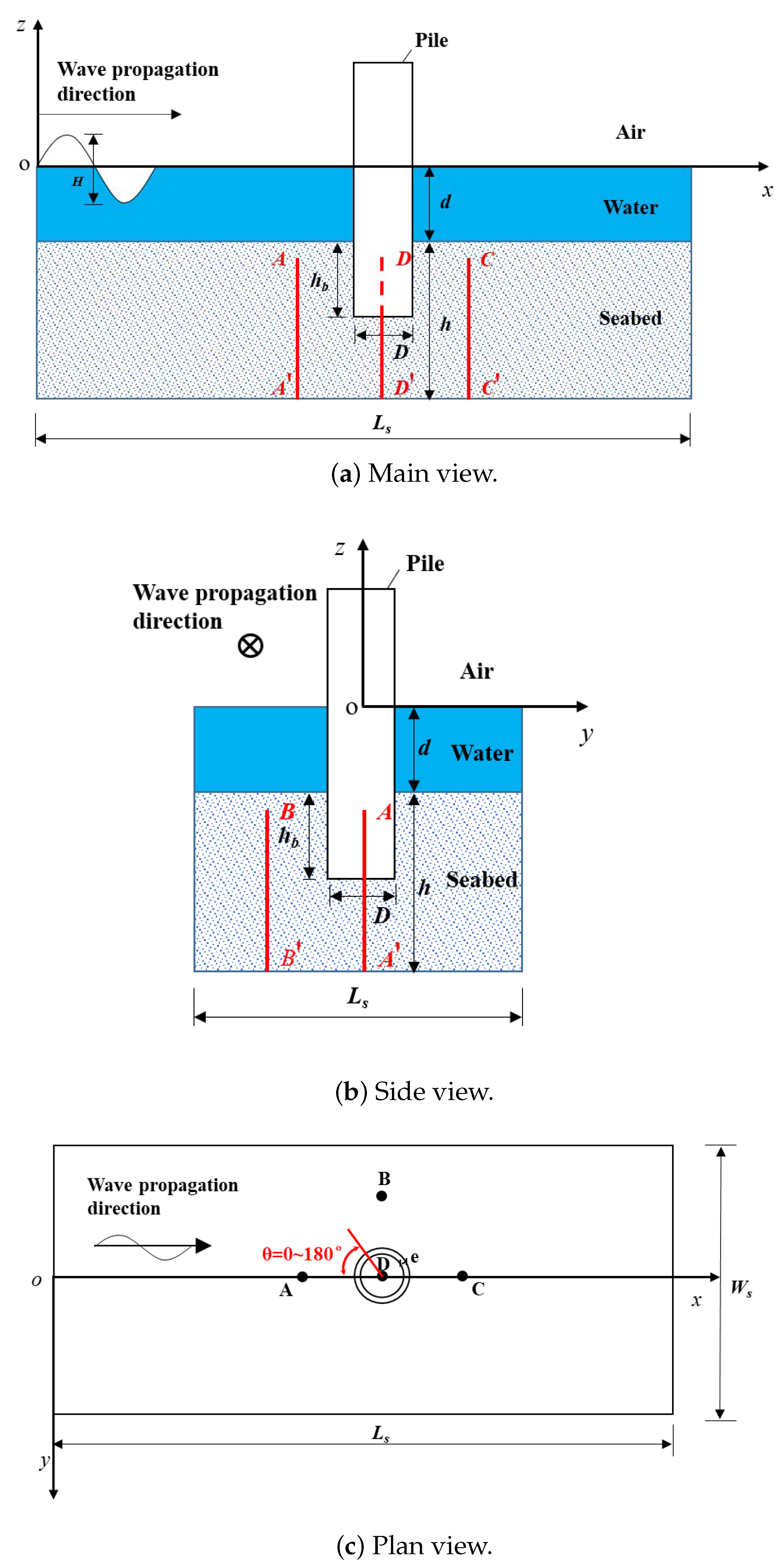
2.3. Computational Domains

Figure 1 shows the hypothetical configuration of the computational domain for the present study. It is noted that the origin of the reference system (e.g., O) is located at the interface between the water and air. Moreover, H is the wave height, d is the water depth, h is the seabed thickness, $h_d$ is the embedded depth of the pile, D is the pile diameter, and e is the wall thickness. $L_s$ is the length of the wave flume, which is equal to three times the wavelength to avoid wave reflection that could arise at the offshore boundary [26]. $W_s$ is the width of the wave flume, which is 10 times the pile diameter. As reported in [27], when the ratio of the width of the structure to the width of the wave flume is less than 0.2, the boundary effect of the flume width can be ignored. Four reference points (i.e., A, B, C and D) were selected for further analysis as reported in the next section. More specifically, the distance between each point and the middle of the pile is equal to 1.5 times the pile’s diameter, and the vertical distance is 1 m below the seabed surface. Among them, Point D is at the center of the bottom of the pile.

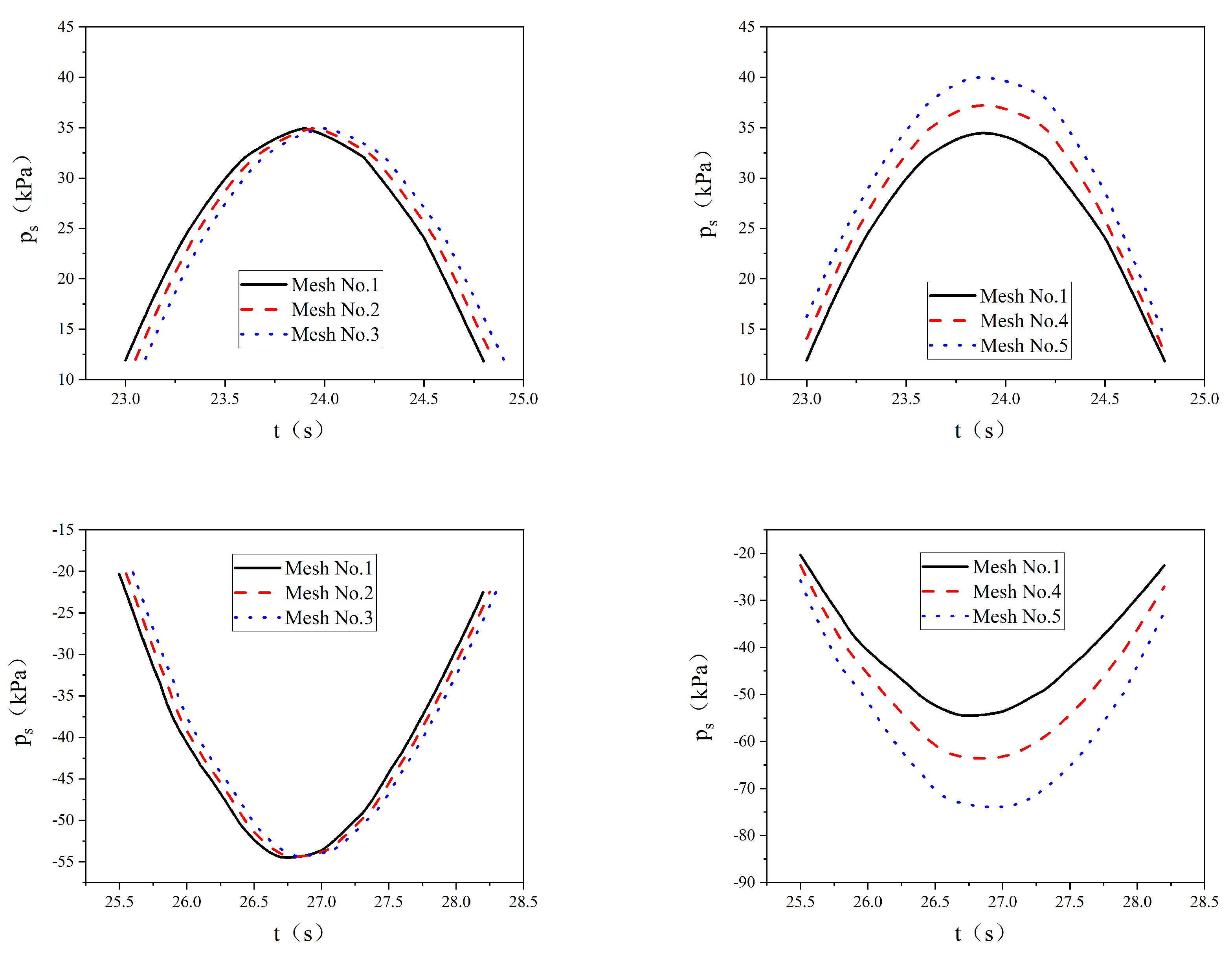
2.4. Numerical Scheme

Generally speaking, the time interval and mesh size used for convergence of wave model are much smaller than that of the seabed model. Nevertheless, to ensure calculation accuracy, this paper adopts a matching time scheme equalling to 0.001 s for these two sub-models and every simulated result is exported at an interval of 0.05 s. On the other hand, the mesh grid is generated by the mesh generation utility blockMesh [28], as shown in Figure 2. The grid sensitivity is analysed through a series of grid convergence tests. The grid sizes of the wave model and the seabed model are shown in the

Table 1. Mesh parameters of wave model.

Mesh No.	$\mathbf{\Delta }\mathit{x}$ = $\mathbf{\Delta }\mathit{y}$	$\mathbf{\Delta }\mathit{z}$	Mesh Number
1	$L_w/150$	H/10	5090160
2	$L_w/100$	H/10	2282880
3	$L_w/50$	H/10	586224
4	$L_w/150$	H/15	76335240
5	$L_w/150$	H/20	10180320

and

Table 2. Mesh parameters of seabed model.

Mesh No.	$\mathbf{\Delta }\mathit{x}$ = $\mathbf{\Delta }\mathit{y}$	$\mathbf{\Delta }\mathit{z}$	Mesh Number
1	$L_w/150$	h/10	5256620
2	$L_w/100$	h/10	4715440
3	$L_w/50$	h/10	1211160
4	$L_w/150$	h/15	10513240
5	$L_w/150$	h/20	15769860

. As can be seen, Figure 3 shows the variation of free water surface $\eta$ with five different meshes over the wave period. Meanwhile, Figure 4 displays the distribution of wave-induced pore pressure $p_s$ with five different meshes near the wave wrest and trough loadings, respectively. By comparing between various mesh sizes, a high calculation accuracy can be observed under the combination of $\Delta x$ = $\Delta y$ = $L_w$/150 plus $\Delta z$ = H/20 and $\Delta x$ = $\Delta y$ = $L_w$/150 plus $\Delta z$ = h/20, which are separately chosen for wave and seabed sub-models. In short, for achieving high computational efficiency, this paper adopts the matching time scheme and the non-matching mesh system during the simulation.

2.5. Boundary Conditions

To solve the flow motion and soil dynamic in the above governing equation, appropriate boundary conditions are employed at the boundaries of these two sub-domains and the surface of the open-ended pile (see Figure 5).

• Wave model: at x = 0, the velocity profile U and the volume fraction $\alpha$ are imposed based on fifth-order wave theory [29] in this work; at x = $L_s$, an active wave absorption technique works by constantly adjusting the boundary conditions with a correction velocity and a corrected phase fraction for removing the wave reflection.
• Seabed model: at z = $-d$, we have ${\sigma }_s^{\prime }=0,{\tau }_s=0,p_s=p_w$; an impermeable boundary condition, $u_s=v_s=w_s=\frac{\partial p_s}{\partial z}=0$, is applied at z = $-(d+h)$; similarly, a fixed wall boundary condition, $u_s=v_s=\frac{\partial p_s}{\partial n}=0$, is adopted at the lateral sides of the computational domain; in terms of the boundary between the pile and the seabed, we assume that the soil skeleton and the structure move synchronously, i.e., $u_s=u_p,{\tau }_s={\tau }_p$.

2.6. Integration of Wave and Seabed Models

Since the wave-induced amplitude of structural vibration and soil deformation is smaller than the wavelength, a one-way coupling algorithm is considered in the dynamic FSSI analysis. Based on the input data, including the wave and seabed parameters, the wave model is executed to obtain the flow field characteristics at each time step. The wave pressure at the bottom of the obtained wave model is applied to the seabed surface through an in-house data exchange port. The seabed model is executed to obtain the characteristics of the wave-induced seabed response (i.e., pore water pressure, effective stress and seabed displacement, etc.), and export the pre-defined numerical results. Overall, Figure 6 illustrates the one-way coupling process of the wave-seabed-structure interactions intuitively.

3. Model Validation

In this section, the present model is validated with the existing published experimental data [10,30,31,32] (see Figure 7) for wave and seabed model, respectively. Moreover, the wave and soil properties of these mentioned experiments are listed in

Table 3. Parameters for verification of wave model.

	No.	H [m]	T [s]	d [m]	D [m]
Umeyama [30]
	W1	0.0103	1	0.3	[-]
	W2	0.0234	1	0.3	[-]
	W3	0.0361	1	0.3	[-]
Zang et al. [31]
	R2	0.14	1.22	0.505	0.25
	R3	0.12	1.63	0.505	0.25

and

Table 4. Parameters for verification of seabed model.

	H [m]	T [s]	d [m]	h [m]	${\mathit{S}}_{\mathit{r}}$ [-]	G [N/m2]	$\mathit{\mu }$ [-]	${\mathit{k}}_{\mathit{s}}$ [m/s]
Chang et al. [32]
	0.25	2	0.562	0.6	1	10${}^7$	0.12	2.11 × 10${}^{-5}$
Wang et al. [10]
	0.1	1.4 & 2	0.6	1	1	8.85 × 10${}^7$	0.3	2.382 × 10${}^{-5}$

. As far as the authors know, there is no flume test for wave-induced excess pore-pressure around an open-ended pile. Therefore, the existing experiment including a solid pile is chosen in the following model verification.

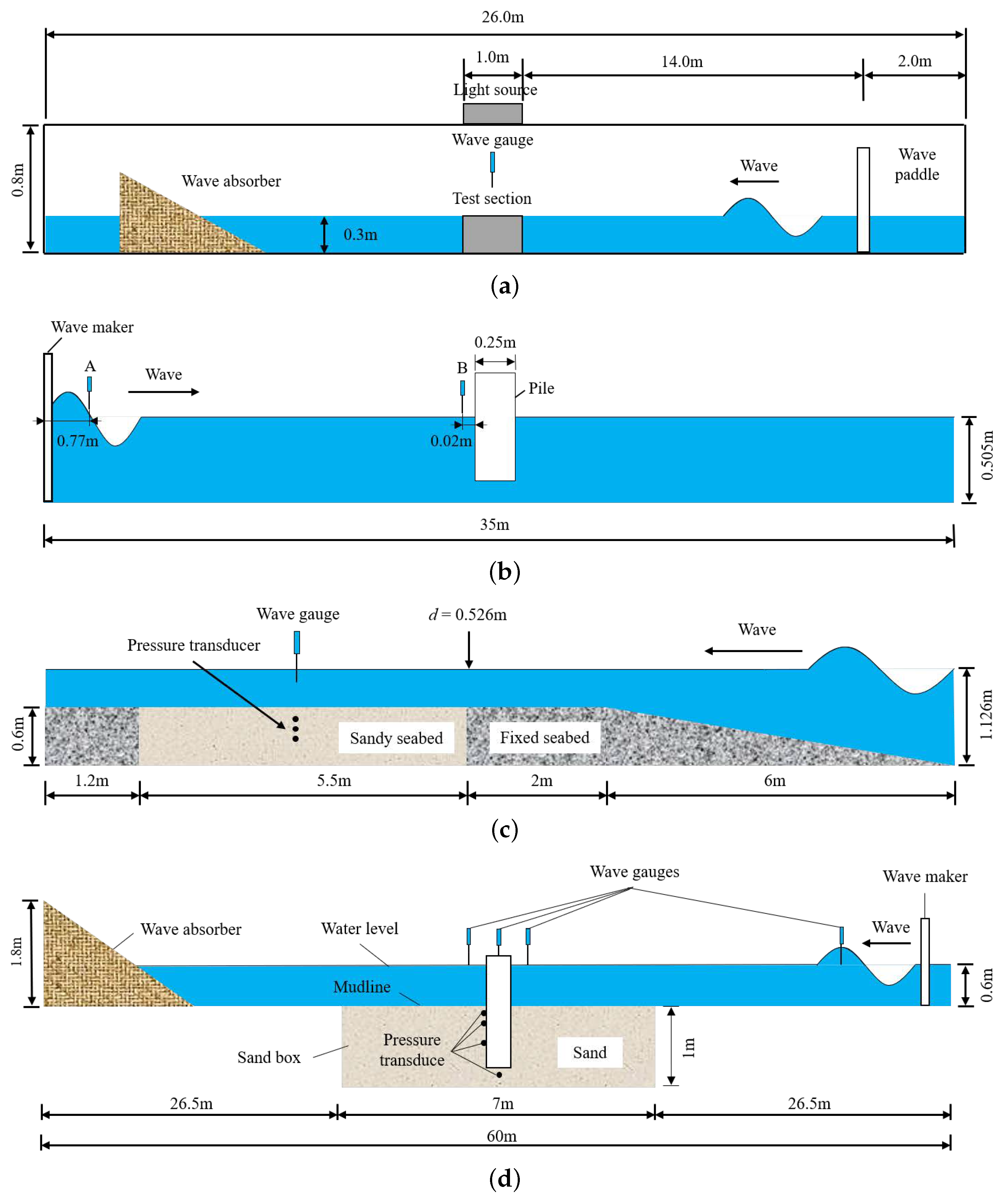
3.1. Wave Model Verification

3.1.1. Verification of Wave Model without a Structure

Umeyama [30] experimentally analysed the hydrodynamic characteristics of ocean waves and currents in a wave flume. This paper does not consider the effect of ocean currents on the seabed response. In all experimental conditions, the water depth and wave period are constant values of 30 cm and 1.0 s, respectively. The wave profile ($\eta$) of their cases W1–W3 was used for comparison, in which the regular wave heights were 1.03 cm, 2.34 cm, and 3.61 cm, respectively. Figure 8 shows the comparison results and setup of the experimental system [30]. As seen, the experimental data and numerical results of free water surface ($\eta$) are generally consistent with each other. The difference between the experimental data and the simulation results may be due to the fact that the bottom boundary condition of the velocity is set to 0 and the water depth in the experiment is relatively shallow.

3.1.2. Verification of Wave Model with a Structure

Zang et al. [31] performed a number of flume tests to study the non-linear interaction between waves and vertical cylinders. As shown in Figure 9a–c, the numerical results at two different points under different wave conditions agree well with the experimental data, showing the “jumping” behaviour of the wave trough in front of the single pile. Generally speaking, this FVM model can effectively capture the variation of $\eta$ near the structure. The difference between the experimental results and the numerical ones can be attributed to the assumption of incompressible fluid in the model, and the appearance of entrained bubbles during the interaction of waves and structures in physical experiments will generate the dissipation of wave energy.

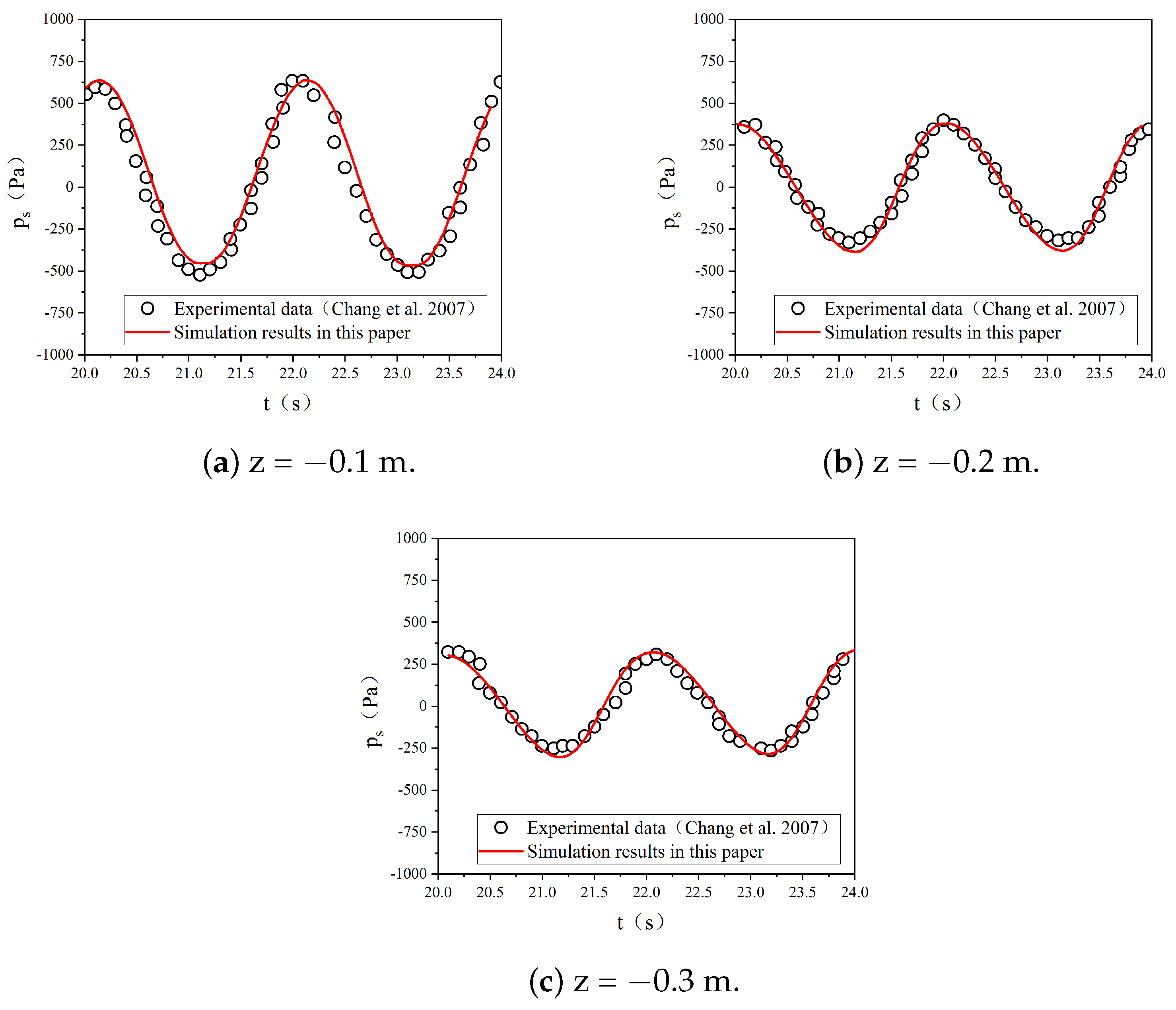
3.2. Seabed Model Verification

3.2.1. Validation of Seabed Model without a Structure

Chang et al. [32] conducted a series of hydraulic model tests on a movable bed within a wave flume with a length of 100 m, a width of 1.5 m and a height of 2 m (see Figure 7c). For model validation, the experimental data of wave-induced pore water pressure at different soil depth is used for comparison (see Figure 10). It can be seen that a good agreement is obtained, indicating that the coupled FVM model can effectively simulate the wave-induced non-linear seabed response.

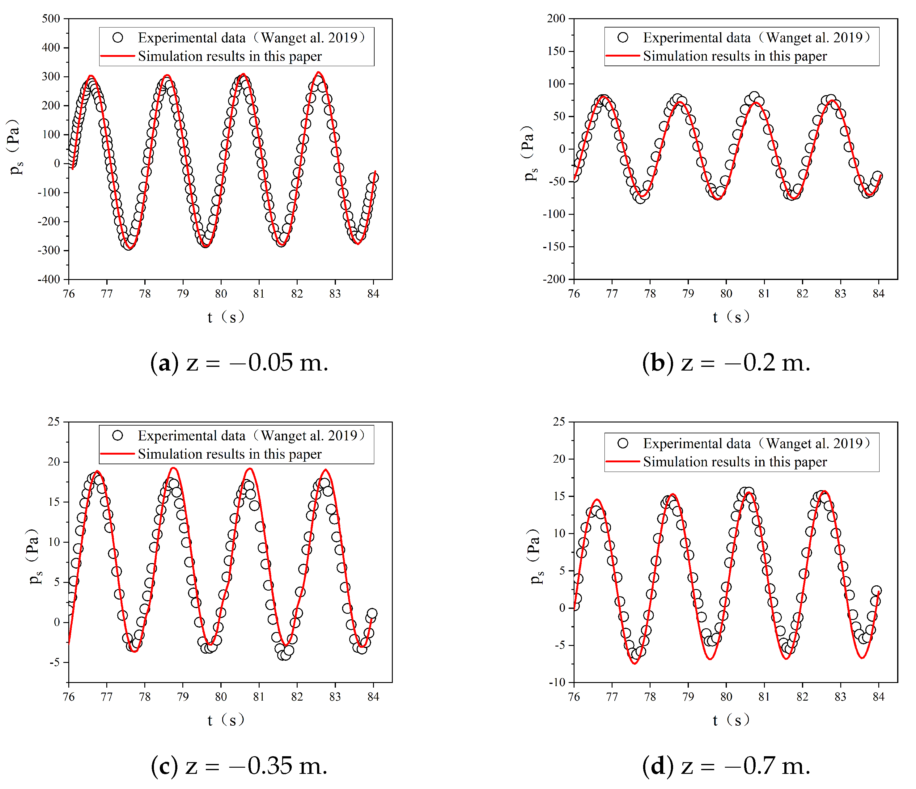
3.2.2. Verification of Seabed Model with a Structure

Wang et al. [10] presented a train of wave flume tests in the specially-designed flume (60.0 m × 1.8 m × 2.0 m), as shown in Figure 7d. The comparison results in terms of the pore water pressure around a single pile at various soil depths are displayed in Figure 11. It is worth noting that the numerical results from the FVM model generally agree with the experimental data. This can ensure that subsequent studies on the seabed response caused by waves around the open-ended piles can be carried out accurately.

4. Results And Discussion

The focus of this research is to numerically evaluate the stability of the seabed foundation around the open-ended pile. Therefore, a series of parametric studies have been conducted to discuss the influence of wave, seabed and pile characteristics on the development of seabed response near the structure. For more information,

Table 5. Model verification wave seabed parameters.

	Parameter	Value	Unit
Wave	Regular wave height (H)	6, 8, 10	m
	Regular wave period (T)	6, 8, 10	s
	Water depth (d)	15, 17, 20	m
Seabed	Seabed thickness (h)	18	m
	Degree of saturation ($S_r$)	0.93, 0.95, 0.97	-
	Shear modulus (G)	10${}^7$	N/m${}^2$
	Poisson’s ratio ($\mu$)	0.33	-
	Porosity ($n_s$)	0.425	-
	Soil permeability ($k_s$)	10${}^{-3}$, 5 × 10${}^{-4}$, 10${}^{-4}$	m/s
Open-ended pile	Pile diameter (D)	4, 5, 6	m
	Buried depth ($h_b$)	8	m
	Pipe wall (e)	0.04	m

summarizes the input data used in this study.

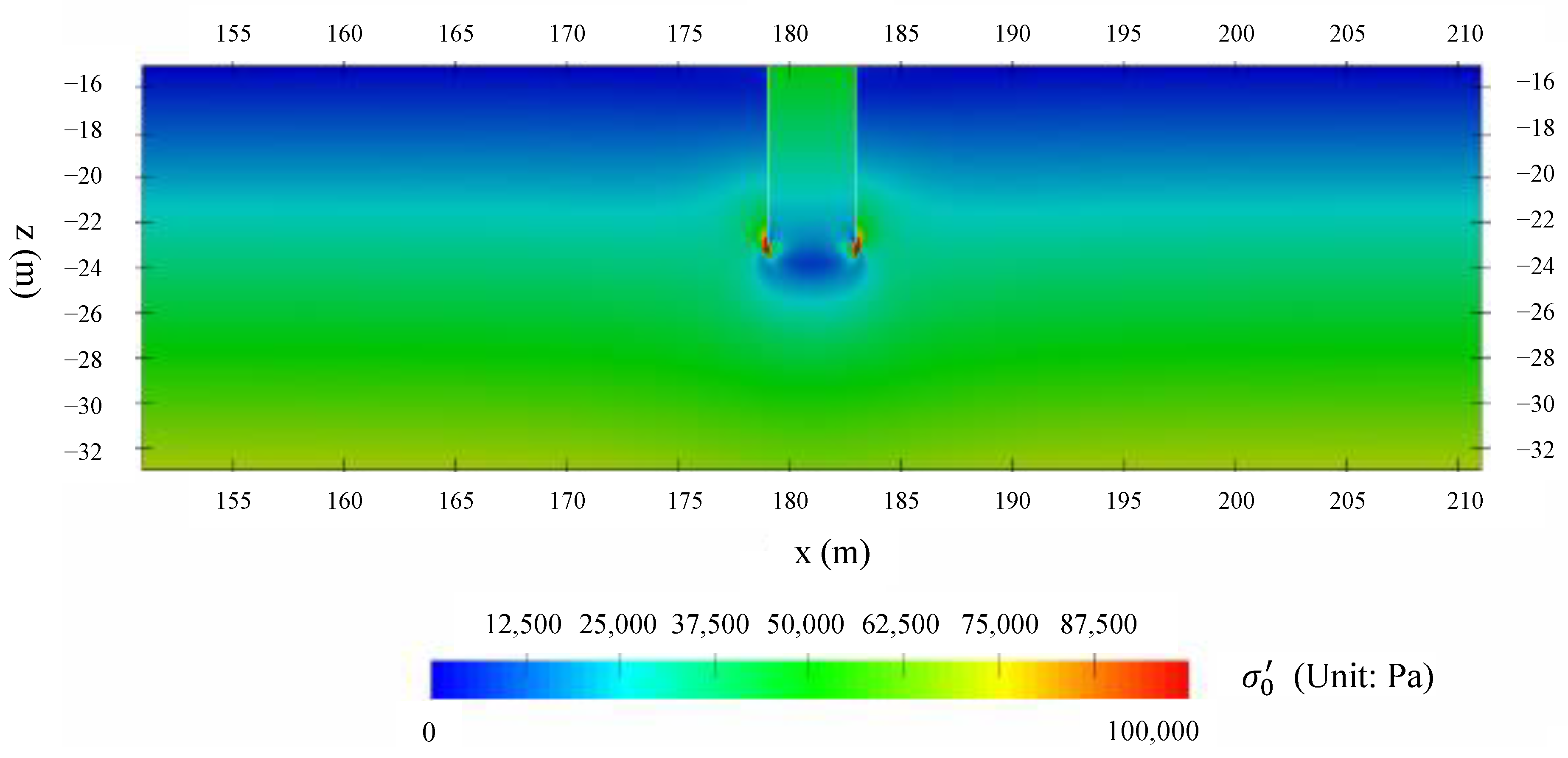
4.1. Seabed Consolidation

In the natural environment, the seabed experiences a consolidation process for a long period. However, the construction process of the offshore wind turbine foundation will inevitably cause disturbances to the surrounding seabed. As a result, the seabed will reach a new equilibrium state on the basis of the original static load consolidation.

Therefore, in this study, taking the effective stress ${\sigma }_0^{\prime }$ of the seabed into consideration as the initial condition, the wave–seabed structure interactions are further analysed. Note that ${\sigma }_0^{\prime }=({\sigma }_{x0}^{\prime }+{\sigma }_{y0}^{\prime }+{\sigma }_{z0}^{\prime })/3$, where ${\sigma }_{x0}^{\prime }$, ${\sigma }_{y0}^{\prime }$ and ${\sigma }_{z0}^{\prime }$ represent the initial effective stress in the x-, y- and z- direction, respectively. Figure 12 shows the distribution of the effective stress of seabed around the open-ended pile after completeness of consolidation. It can be seen from the figure that the effective stress of the seabed gradually increases with the increase in soil depth, and the phenomenon of stress concentration appears at the bottom of the pile. In the inner area of the pile, the effective stress first increases and then decreases with the increase in soil depth. The reduction of the effective stress inside the pile may be induced by the numerical model based on the elastic deformation theory and the thinner pile wall. This could further result in the occurrence of stress concentration at the bottom of the pile, while the stress near the centre of the pipe pile is smaller.

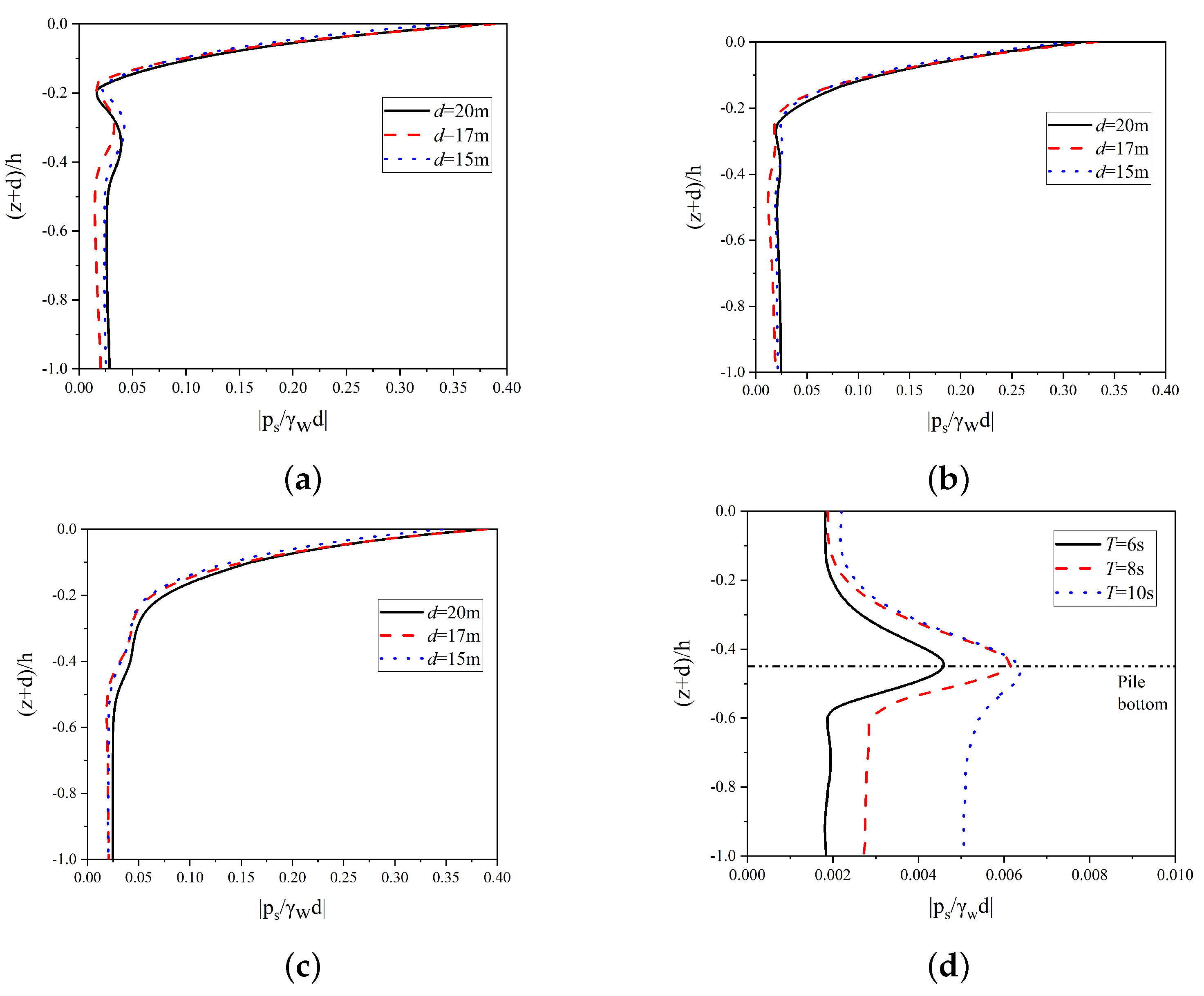
4.2. Influence of Wave Characteristics on the Transient Soil Response around the Open-Ended Pile

Figure 13, Figure 14 and Figure 15 display the curves of the maximum dimensionless wave-induced pore water pressure ($|p_s/{\gamma }_{w}d|$, where $p_s$: the wave-induced pore water pressure; ${\gamma }_w$: the unit weight of the pore water; and d: water depth) at each measuring point (see Figure 1c) as a function of soil depth under different wave conditions. As seen, the wave-induced pore water pressure around the pile is approximately linearly distributed along with the soil depth in the shallow layer of the seabed. In general, due to the gradual dissipation of pore water pressure, the maximum pore water pressure induced by waves and its attenuation rate decreases with increasing soil depth. Especially when $(z+d)/h$<0.2 (where z is the position coordinate of soil depth relative to the mean water level, and its value is negative downward), this trend is more pronounced. On the contrary, the value of $|p_s/{\gamma }_{w}d|$ inside the open-end pipe pile gradually increases with the increase in soil depth, until it reaches the maximum value at the bottom of the pile (i.e., $(z+d)/h$≈0.45). Lin et al. [18] obtained similar conclusions by analysing the wave-induced seabed response at the bottom of a single pile. Thus, this can be explained by the fact that there is no wave pressure on the seabed surface inside the open-ended pile as well as the upward penetration of the pore water pressure near the pile bottom.

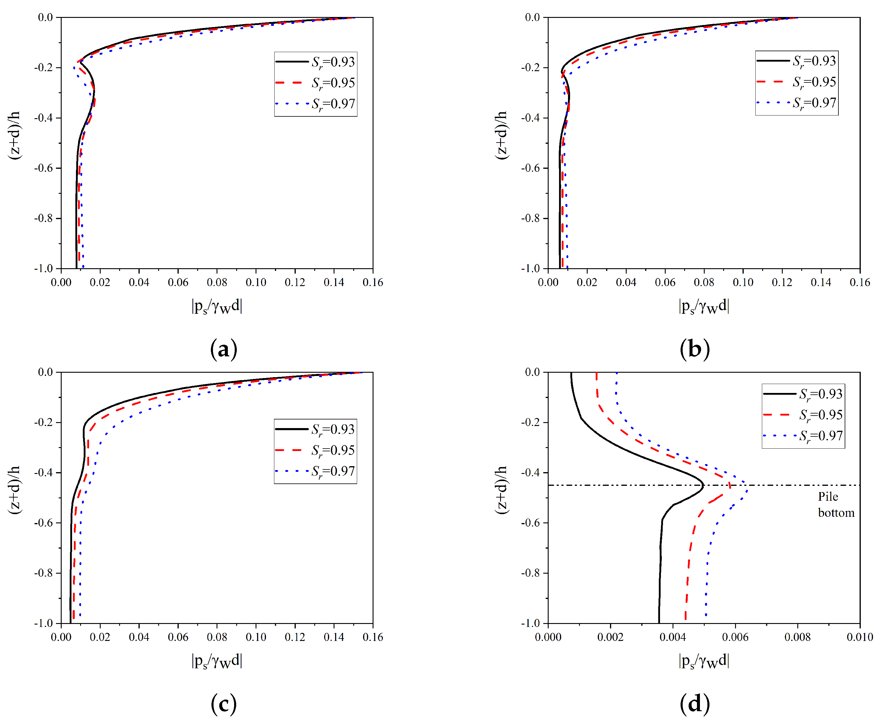
4.3. Influence of Seabed Characteristics on Transient Soil Response around the Open-Ended Pile

Figure 16 indicates that the wave-induced pore water pressure ($|p_s/{\gamma }_{w}d|$) on the wave-facing side of the pile is greater than that in other directions, and its attenuation rate gradually decreases with the increase in soil permeability. This kind of attenuation is more significant in the upper half of the pile, resulting from the amplitude damping and phase lag of transient pore water pressure in the porous seabed [33]. In addition, the ($|p_s/{\gamma }_{w}d|$) inside the open-ended pile increases gradually as the soil depth increases, reaches the maximum at the bottom of the pile, and then gradually decreases to a fixed value. From the perspective of the effect of degree of saturation, it can be observed that the greater the degree of saturation, the smaller the attenuation rate of pore water pressure as the soil depth increases, as shown in Figure 17. In contrast, the degree of saturation has little effect on the pore water pressure. However, its influence gradually becomes obvious with increasing soil depth at vertical line C–C′. Similarly, the pore water pressure inside the open-ended pile gradually increases as the soil depth increases, and it reaches the maximum value at the pile bottom.

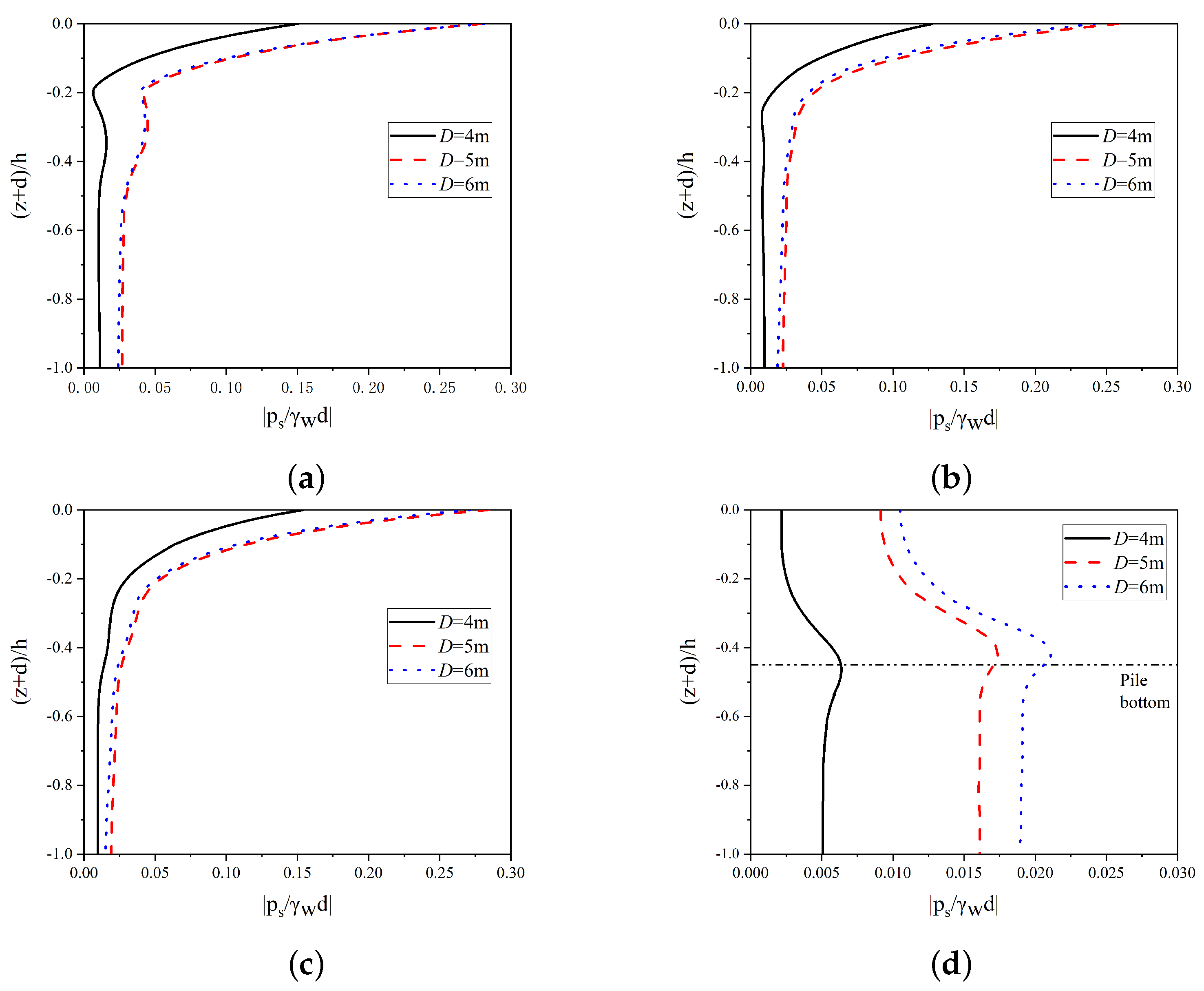
4.4. Influence of Pile Characteristics on Transient Soil Response around the Open-Ended Pile

Figure 18 presents the curves of the maximum wave-induced pore water pressure ($|p_s/{\gamma }_{w}d|$) at each measuring point along with the soil depth for various pile diameters. As can be seen, the wave-induced pore water pressure around the pile body gradually decreases as the soil depth increases. However, it increases first and then decreases inside the open-ended pile. In addition, near the surface of the seabed, the pile diameter has little effect on the pore pressure. However, as the soil depth increases, the pore water pressure increases as the pile diameter increases, and this effect becomes more evident. On the other hand, it can be inferred that increasing pile diameter has an evident blocking effect on the wave propagation from the front face to the back face of the pile foundation. This could widen the difference between the free water surface and the static water surface around the pile, which in turn will cause greater wave pressure on the seabed surface. As for the varying rate of pore pressure along with the soil depth, the numerical results show that the wave-induced pore pressure at three points (i.e., Point A, B and C) decreases significantly as the pile diameter decreases; meanwhile, in the interior of the pipe pile (i.e., point D), the wave-induced pore pressure increases faster with a smaller pile diameter until reaching the pile bottom. However, a greater value of $|p_s/{\gamma }_{w}d|$ can be obtained with a larger pile diameter.

4.5. Influence of Environmental and Structural Characteristics on Transient Soil Liquefaction around the Open-Ended Pile

When there are structures on the seabed, the nearby seabed foundation will reach a consolidated state for a period of time under the self-weight of the soil and the structure, which will cause the pore water pressure in the seabed to attenuate and the soil effective stress to increase. To this end, the liquefaction condition in the seabed foundation is evaluated based on the liquefaction criterion proposed by Zhao et al. [34]:

$${\sigma }_0^{\prime }\le p_s-p_{w0}$$

(12)

in which $p_{w0}$ is dynamic wave pressure at the seabed surface and ${\sigma }_0^{\prime }$ is the mean initial effective stress after pre-consolidation. It should be noted that since the average effective stress of the seabed cannot be measured on-site, this liquefaction standard cannot be used in actual working conditions. However, the transient seafloor liquefaction can be evaluated based on this criterion through numerical results.

The distribution of the transient soil liquefaction depth ($d_L$) around the open-ended pile is shown in Figure 19. Notably, the maximum value of $d_L$ can be observed around the specific location when $\theta$ = 90${}^{\circ }$ (i.e., the lateral sides of the mono-pile). In short, as the wave height and period increase, $d_L$ increases positively. As the water depth, degree of saturation, and soil permeability increase, it increases negatively. Please note that the maximum value of $d_L$ under various conditions is adopted for comparison in the following discussion. More specifically, when the wave height increases from 6 m to 10 m, $d_L$ increases by 0.42 m; when the wave period increases from 6 s to 10 s, $d_L$ increases by 1.35 m; when the water depth increases from 15 m to 20 m, $d_L$ decreases by 0.26 m; when the saturation increases from 93% to 97%, $d_L$ decreases by 0.22 m; when the soil permeability increases from 1 × 10${}^{-4}$ to 1 ×10${}^{-3}$ m/s, $d_L$ decreases by 0.11 m; when the pile diameter increases from 4 m to 6 m, $d_L$ decreases by 0.72 m. By contrast, the wave period has the greatest influence on $d_L$ among the five elements of the environmental characteristic. Nevertheless, the influence of pile diameter on $d_L$ cannot be ignored. On the other hand, $d_L$ at $\theta$ = 90${}^{\circ }$ is greater than that at the front and back of the pile (i.e., $\theta$ = 0${}^{\circ }$ and 180${}^{\circ }$).

5. Conclusions

Based on the established three-dimensional numerical model of wave-open-ended pile–seabed interactions, this paper analyses the influence of wave characteristics, seabed characteristics and pile geometrical characteristics on the seabed dynamics around the piles. The conclusions are as follows:

(1) The wave-induced pore water pressure decreases as the soil depth increases. The existence of the pile foundation significantly alters the development of seabed response. This leads to the largest pore water pressure being on the wave-facing side of the open-ended pile compared to other locations.

(2) The numerical results show that the largest value of $d_L$ can be observed at $\theta$=90${}^{\circ }$. Among the three elements of wave characteristics, the wave period has the greatest influence on the $d_L$, followed by wave height, and water depth has the least influence on it. Compared with the degree of saturation, the soil permeability has a greater impact on $d_L$. The influence of pile diameter on $d_L$ cannot be ignored as well.

(3) Compared with previous research results of solid piles, the pore water pressure around open-ended piles varies with soil depth in the same way. The pore water pressure inside the pile reaches its maximum value at the bottom of the pile, but decreases in the vertical direction on both sides. In addition, as the soil depth increases, the distribution trend of pore water pressure in the inner zone of the pile presents a “V” shape rotated 90 degrees counterclockwise. This implies a greater value of pore water pressure at the bottom of the pile, resulting in seabed residual liquefaction due to the accumulated pore pressure under the cyclic wave loading. Other than this, the existing FSSI experiments on monopile structures show a kind of solid structure rather than open-ended ones. Therefore, future experimental studies need to take this into consideration and provide more complete data for model verification.

References

1. Sumer, B.M. Liquefaction around Marine Structures; World Scientific: Hackensack, NJ, USA, 2014. [Google Scholar]
2. Sumer, B.M.; Fredsøe, J. The Mechanics of Scour in the Marine Environment; World Scientific Publishing Co. Pte. Ltd.: Hackensack, NJ, USA, 2002. [Google Scholar]
3. Jeng, D.S. Mechanics of Wave-Seabed-Structure Interactions: Modelling, Processes and Applications; Cambridge University Press: Cambridge, UK, 2018. [Google Scholar] [CrossRef]
4. Li, Y.; Ong, M.C.; Tang, T. Numerical analysis of wave-induced poro-elastic seabed response around a hexagonal gravity-based offshore foundation. Coast. Eng. 2018, 136, 81–95. [Google Scholar] [CrossRef]
5. Celli, D.; Li, Y.; Ong, M.C.; Di Risio, M. Random wave-induced momentary liquefaction around rubble mound breakwaters with submerged berms. J. Mar. Sci. Eng. 2020, 8, 338. [Google Scholar] [CrossRef]
6. Biot, M.A. General theory of three-dimensional consolidation. J. Appl. Phys. 1941, 26, 155–164. [Google Scholar] [CrossRef]
7. Chang, K.T.; Jeng, D.S. Numerical study for wave-induced seabed response around offshore wind turbine foundation in Donghai offshore wind farm, Shanghai, China. Ocean Eng. 2014, 85, 32–43. [Google Scholar] [CrossRef]
8. Zhang, C.; Zhang, Q.; Wu, Z.; Zhang, J.; Sui, T.; Wen, Y. Numerical study on effects of the embedded monopile foundation on local wave-induced porous seabed response. Math. Probl. Eng. 2015, 184621. [Google Scholar] [CrossRef] [Green Version]
9. Zhang, C.; Sui, T.; Zheng, J.; Xie, M.; Nguyen, V.T. Modelling wave-induced 3D non-homogeneous seabed response. Appl. Ocean Res. 2016, 61, 101–114. [Google Scholar] [CrossRef]
10. Wang, S.; Wang, P.; Zhai, H.; Zhang, Q.; Chen, L.; Duan, L.; Liu, Y.; Jeng, D.S. Experimental study for wave-induced pore water pressures in a porous seabed around a mono-pile. J. Mar. Sci. Eng. 2019, 7, 237. [Google Scholar] [CrossRef] [Green Version]
11. Qi, W.G.; Gao, F.P. Physical modelling of local scour development around a large-diameter monopile in combined waves and current. Coast. Eng. 2014, 83, 72–81. [Google Scholar] [CrossRef] [Green Version]
12. Chen, L.; Zhai, H.; Wang, P.; Jeng, D.S.; Zhang, Q.; Wang, S.; Duan, L.; Liu, Y. Physical modeling of combined waves and current propagating around a partially embedded monopile in a porous seabed. Ocean Eng. 2020, 205, 107307. [Google Scholar] [CrossRef]
13. Zhang, Q.; Zhai, H.; Wang, P.; Wang, S.; Duan, L.; Chen, L.; Liu, Y.; Jeng, D.S. Experimental study on irregular wave-induced pore water pressures in a porous seabed around a mono-pile. Appl. Ocean Res. 2020, 95, 102041. [Google Scholar] [CrossRef]
14. Li, C.; Gao, F.; Yang, L. Breaking-wave induced transient pore pressure in a sandy seabed: Flume modeling and observations. J. Mar. Sci. Eng. 2021, 9, 160. [Google Scholar] [CrossRef]
15. Li, X.; Gao, F.; Yang, B.; Zang, J. Wave-induced pore pressure response and soil liquefaction around pile foundation. Int. J. Offshore Polar Eng. 2011, 21, 233–239. [Google Scholar]
16. Sui, T.; Zhang, C.; Guo, Y.; Zheng, J.; Jeng, D.S.; Zhang, J.; Zhang, W. Three-dimensional numerical model for wave-induced seabed response around mono-pile. Ships Offshore Struct. 2016, 11, 667–678. [Google Scholar] [CrossRef] [Green Version]
17. Sui, T.; Zheng, J.; Zhang, C.; Jeng, D.S.; Zhang, J.; Guo, Y.; He, R. Consolidation of unsaturated seabed around an inserted pile foundation and its effects on the wave-induced momentary liquefaction. Ocean Eng. 2017, 131, 308–321. [Google Scholar] [CrossRef] [Green Version]
18. Lin, Z.; Pokrajac, D.; Guo, Y.; Jeng, D.s.; Tang, T.; Rey, N.; Zheng, J.; Zhang, J. Investigation of nonlinear wave-induced seabed response around mono-pile foundation. Coast. Eng. 2017, 121, 197–211. [Google Scholar] [CrossRef] [Green Version]
19. Duan, L.; Jeng, D.S.; Wang, D. PORO–FSSI–FOAM: Seabed response around a mono-pile under natural loadings. Ocean Eng. 2019, 184, 239–254. [Google Scholar] [CrossRef]
20. Abdelkader, A.; El Naggar, M.H. Hybrid foundation system for offshore wind turbine. Geotech. Geol. Eng. 2018, 36, 2921–2937. [Google Scholar] [CrossRef]
21. Jeng, D.S.; Ye, J.H.; Zhang, J.S.; Liu, P.L.-F. An integrated model for the wave-induced seabed response around marine structures: Model verifications and applications. Coast. Eng. 2013, 72, 1–19. [Google Scholar] [CrossRef]
22. Liang, Z.; Jeng, D.S. PORO–FSSI–FOAM model for seafloor liquefaction around a pipeline under combined random wave and current loading. Appl. Ocean Res. 2021, 107, 102497. [Google Scholar] [CrossRef]
23. Higuera, P.; Lara, J.L.; Losada, I.J. Realistic wave generation and active wave absorption for Navier-Stokes models: Application to OpenFOAM. Coast. Eng. 2013, 71, 102–118. [Google Scholar] [CrossRef]
24. Higuera, P.; Buldakov, E.; Stagonas, D. Simulation of Steep Waves Interacting with a Cylinder by Coupling CFD and Lagrangian Models. Int. J. Offshore Polar Eng. 2021, 31, 87–94. [Google Scholar] [CrossRef]
25. Verruijt, A. Flow Through Porous Media; Chapter Elastic Storage of Aquifers; Academic Press: London, UK, 1969; pp. 331–376. [Google Scholar]
26. Ye, J.; Jeng, D.S. Response of seabed to natural loadin: Waves and current. J. Eng. Mech. 2012, 138, 601–613. [Google Scholar] [CrossRef]
27. Chakrabarti, S.K. Offshore Structure Modeling; World Scientific Publishing Co. Pte. Ltd.: Hackensack, NJ, USA, 1994. [Google Scholar]
28. Greenshields, C.J.; OpenFOAM v9 User Guide. The OpenFOAM Foundation. 2017. Available online: https://cfd.direct/openfoam/user-guide (accessed on 12 October 2021).
29. Skjelbreia, L.; Hendrickson, J.A. Fifth order gravity wave theory. Proceedings of 7th International Conference on Coastal Engineering, Mexico City, Mexico, 29 January 1960; pp. 184–196. [Google Scholar]
30. Umeyama, M. Coupled PIV and PTV measurements of particle velocities and trajectories for surface waves following a steady current. J. Waterw. Port, Coast. Ocean Eng. 2011, 137, 85–94. [Google Scholar] [CrossRef]
31. Zang, J.; Taylor, P.H.; Morgan, G.; Stringer, R.; Orszaghova, J.; Grice, J.; Tello, M. Steep wave and breaking wave impact on offshore wind turbine foundations–ringing re-visited. In Proceedings of the 25th International Workshop on Water Waves and Floating Bodies, Harbin, China, 9–12 May 2010; pp. 9–12. [Google Scholar]
32. Chang, S.C.; Lin, J.G.; Chien, L.K.; Chiu, Y.F. An experimental study on non-linear progressive wave-induced dynamic stresses in seabed. Ocean Eng. 2007, 34, 2311–2329. [Google Scholar] [CrossRef]
33. Yamamoto, T.; Koning, H.; Sellmeijer, H.; Hijum, E.V. On the response of a poro-elastic bed to water waves. J. Fluid Mech. 1978, 87, 193–206. [Google Scholar] [CrossRef]
34. Zhao, H.Y.; Jeng, D.S.; Liao, C.C.; Zhu, J.F. Three-dimensional modeling of wave-induced residual seabed response around a mono-pile foundation. Coast. Eng. 2017, 128, 1–21. [Google Scholar] [CrossRef]
Figure 1. Schematic diagram of wave–pile–seabed interaction model.
Jmse 09 01238 g001
Figure 2. FVM mesh used in computation of the seabed and open-ended pile.
Jmse 09 01238 g002
Figure 3. Free surface elevation ( η ) over time for different mesh schemes (when H = 4.2 m, T = 6.2 s, d = 15 m, and L w = 58.8 m).
Jmse 09 01238 g003
Figure 4. Wave-induced pore pressure ( p s ) over time for different mesh schemes (when S r = 0.99, G = 10 7 Pa, μ = 0.3, n = 0.448, k s = 2.382 × 10 5 m/s, and h = 15 m).
Jmse 09 01238 g004
Figure 5. Schematic diagram of the boundary conditions of the wave model and the seabed model.
Jmse 09 01238 g005
Figure 6. One-way coupling algorithm of FSSI simulation.
Jmse 09 01238 g006
Figure 7. Experimental set-up of (a) Umeyama [30]; (b) Zang et al. [31]; (c) Chang et al. [32]; (d) Wang et al. [10].
Jmse 09 01238 g007
Figure 8. Comparison of numerical results of wave profile with experimental data [30]. Note: z = 0 denotes the mean water level in the experiments.
Jmse 09 01238 g008
Figure 9. Comparison of numerical results of wave profile with experimental data [31]. Note: z = 0 denotes the mean water level in the experiments.
Jmse 09 01238 g009
Figure 10. Comparison of the numerical results of the maximum pore water pressure along the soil depth with the experimental data [32]. Note: z = 0 denotes the seabed surface in the experiments.
Jmse 09 01238 g010
Figure 11. Comparison of numerical results of wave-induced pore water pressure at various soil depths with experimental data [10]. Note: z = 0 denotes the seabed surface in the experiments.
Jmse 09 01238 g011
Figure 12. The distribution of the effective stress around the open-end pipe pile after seabed consolidation.
Jmse 09 01238 g012
Figure 13. Curves of the maximum pore water pressure with different wave height along vertical lines: (a) A–A′; (b) B–B′; (c) C–C′; (d) D–D′. (Test positions are given in Figure 1).
Jmse 09 01238 g013
Figure 14. Curves of the maximum pore water pressure with different wave period along vertical lines: (a) A–A′; (b) B–B′; (c) C–C′; (d) D–D′.
Jmse 09 01238 g014
Figure 15. Curves of the maximum pore water pressure with different water depth along vertical lines: (a) A—A′; (b) B—B′; (c) C—C′; (d) D—D′.
Jmse 09 01238 g015
Figure 16. Curves of the maximum pore water pressure with different soil permeability along vertical lines: (a) A–A′; (b) B–B′; (c) C–C′; (d) D–D′.
Jmse 09 01238 g016
Figure 17. Curves of the maximum pore water pressure with different degree of saturation along vertical lines: (a) A–A′; (b) B–B′; (c) C–C′; (d) D–D′.
Jmse 09 01238 g017
Figure 18. Curves of the maximum pore water pressure with different pile diameter along vertical lines: (a) A–A′; (b) B–B′; (c) C–C′; (d) D–D′.
Jmse 09 01238 g018
Figure 19. The distribution of seabed liquefaction depth at each measuring point vs different wave, seabed and pipe pile characteristics.
Jmse 09 01238 g019