A Wind–Wave-Dependent Sea Spray Volume Flux Model Based on Field Experiments

Abstract

Sea spray can contribute significantly to the exchanges of heat and momentum across the air–sea interface. However, while critical, sea spray physics are typically not included in operational atmospheric and oceanic models due to large uncertainties in their parameterizations. In large part, this is because of the scarcity of in-situ sea spray observations which prevent rigorous validation of existing sea spray models. Moreover, while sea spray is critically produced through the fundamental interactions between wind and waves, traditionally, sea spray models are parameterized in terms of wind properties only. In this study, we present novel in-situ observations of sea spray derived from a laser altimeter through the adoption of the Beer–Lambert law. Observations of sea spray cover a broad range of wind and wave properties and are used to develop a wind–wave-dependent sea spray volume flux model. Improved performance of the model is observed when wave properties are included, in contrast to a parameterization based on wind properties alone. The novel in-situ sea spray observations and the predictive model derived here are consistent with the classic spray model in both trend and magnitude. Our model and novel observations provide opportunities to improve the prediction of air–sea fluxes in operational weather forecasting models.

1. Introduction

Sea spray comprises small water droplets ejected from the sea surface and is of great significance to weather and climate processes [1]. When sea spray droplets are separated from the wave crest and released into the air, the droplets accelerate towards the local wind speed [2,3,4,5]. In doing so, sea spray extracts momentum from the atmosphere and thus reduces the wind speed near the ocean surface [6]. When the heaviest droplets re-enter the ocean, part of the momentum they gained is transferred directly to the ocean surface [7] and as a result, sea spray can contribute to momentum exchange between the upper ocean and the atmosphere and alter the stability of the air–sea boundary layer [8,9,10,11].

In addition to the effects of sea spray on the air–sea momentum transfer, spray can also impact the air–sea heat flux due to the temperature differences between the droplets and the atmosphere [12]. It was reported that spray induced heat flux contributes to more than 10% of the total air–sea heat flux for near surface wind speeds larger than 12 m s⁻¹, while its contribution would become larger than the air–sea heat flux produced directly at the ocean surface once the wind speed exceeds about 30 m s⁻¹ [13]. Evidently, as sea spray can contribute significantly to the momentum, heat, and water vapor flux exchange between the atmosphere and ocean [4,12,14,15], accurate prediction of how much spray is produced at the air–sea boundary is of critical importance.

Sea spray is typically produced through two different processes: bubble bursting and wind shearing [1]. When waves break, air is entrained into the upper ocean in the form of bubble clouds which rise to the sea surface and burst [16,17]. When the bubble caps burst, small droplets are ejected into the air from the surface film followed by droplets emitted from the central jet that forms after the collapse of the bubble cavity [18,19,20,21]. Larger droplets can, however, be produced when winds are sufficiently strong to tear droplets from the wave crests directly [11,22,23,24]. These droplets are referred to as spume droplets and are generated at a wind speed larger than about 7–11 m s⁻¹ [1].

Many studies have been devoted to understanding and quantifying the different sea spray production processes and have led to a variety of sea spray production models [1,22,24,25,26,27]. These spray models typically determine the amount of water injected into the atmosphere per unit area of ocean surface and per unit time [1]. Monahan, Davidson and Spiel [27] initially proposed a spray model based on measurements in the laboratory using the whitecap coverage method. Andreas [6] followed this approach but included more observations to derive an improved spray model. More recently, Troitskaya, Kandaurov, Ermakova, Kozlov, Sergeev and Zilitinkevich [26] used a high-speed digital video camera to observe sea spray generation process and introduced a “bag-based” spray model. However, despite recent advances in our understanding of sea spray production at a small scale, significant uncertainty remains in the accuracy of these spray models when applied in-situ. For instance, Andreas [28] reviewed more than 10 different spray models and stated that under any given wind condition these models range over six orders of magnitudes. More recently, Veron [1] concluded that while the difference between sea spray prediction models for spray drops smaller than spume (i.e., droplets with a radius smaller than 20 $\mathsf{\mu }\mathrm{m}$) has narrowed, the differences between model predictions for spume droplets remains several orders of magnitude. It is this large uncertainty in sea spray production under full wind speed conditions that restricts the reliable implementation of sea spray spume physics in our weather forecasting models.

One of the foremost reasons for the large variability between sea spray prediction models is the scarcity of sea spray observations in the field [29,30,31,32,33,34,35]. This rarity is because conducting field measurements of sea spray close to the sea surface is challenging due to the harsh marine environment. Even when observations are successfully obtained, such observations are often restricted by the temporal and spatial resolution of the instrumentation [1]. For example, Smith, et al. [36] applied optical counters to quantify sea spray properties inshore waters, but their facilities can only identify water drops with a radius smaller than 25 $\mathsf{\mu }\mathrm{m}$ and under calm weather conditions [36]. Rare field spray observations covering a much wider range of droplet radii were obtained by a suite of sensors installed on wing pylons of an airplane [37]. However, due to safety reasons, these measurements were conducted at 30 m above the mean sea level, thereby restricting observations of spume droplets that typically reside much closer to the ocean surface. As such, given the near-absence of sea spray observations in the field under strong wind conditions, current sea spray models are predominantly derived and validated based on observations obtained in the laboratory [11,26,38,39].

Even though laboratory observations have significantly advanced our physical understanding of the sea spray generation processes, the experimental conditions in the laboratory and field are quite different. Firstly, the wind fetch is typically finite in the laboratory, whereas it is infinite in open water. That is, much more wind energy is imparted to the water surface leading to significantly larger physical scales in the field. We note that this has been substantiated by Nilsson, et al. [40] who indicated that the production of sea spray is critically related to the wind fetch. Moreover, waves in the laboratory are generally unidirectional waves with a narrow spectrum and have a direction of propagation equal to that of the wind, they are, in contrast, random and directional in the field. The two-dimensionality of the wave field can be critical as the amount of spray produced at a wind-following wave crest is surely different from a wave crest propagating in the opposite direction of the wind. This thus stresses the need to incorporate wave properties into the sea spray parameterizations.

Including wave properties into the sea spray models was perhaps initiated by Zhao and Toba [41] who introduced the wind–wave Reynolds number ${\mathrm{Re}}_{\mathrm{w}}$ as an indicator for the onset of white capping and thus spray generation. Zhao, et al. [42] proposed to parameterize ${\mathrm{Re}}_{\mathrm{w}}$ into a sea spray model by characterizing the impacts of waves on the whitecap coverage. Norris, et al. [43], based on the observed eddy covariance sea-spray aerosol flux, forced linear fits of sea-spray aerosol flux to the ${\mathrm{Re}}_{\mathrm{w}}$ and derived a wind–wave sea-spray aerosol source model for small-radius sea spray drops. Ovadnevaite, et al. [44] used a direct fit of the size-dependent sea-spray aerosol flux observations to a wind–wave Reynolds number to provide a sea-spray aerosol flux model capturing different wave states. More recently, Laussac, et al. [45] developed a fetch dependent sea-spray aerosol source model by introducing wave age, whereas Lenain and Melville [37] identified the relevance of both wave age and wave steepness. Nevertheless, despite these developments, it remains challenging to incorporate wave effects into sea spray parameterizations, largely due to the limited size of in-situ datasets of concurrent sea spray, wind and wave observations. Thus, to improve our sea spray predictive models, not only do we need in-situ observations of sea spray, but such observations also need to be obtained concurrently with the properties of the wave field.

The objectives of this study are to (i) measure and determine sea spray generation in-situ and (ii) develop a wave-dependent predictive model across a broad range of wind and wave conditions. To achieve this, we build upon the innovative methodologies of Toffoli, et al. [46] and Ma, et al. [47], and present a large set of in-situ sea spray observations derived from measured laser intensity attenuation using laser altimeters. These observations, measured concurrently with wind and wave field properties, are used to develop a wind–wave-dependent spray volume flux model covering a wide range of wind and wave conditions. Section 2 discusses the methodology used to estimate the sea spray volume flux from laser intensity observations and provides a review of the in-situ experiments. Section 3 presents our observations of the sea spray volume flux and the developed parameterization. A discussion of the instrumentation and the spray induced heat flux is considered in Section 4, followed in Section 5 by the conclusions of this study.

2. Methodology

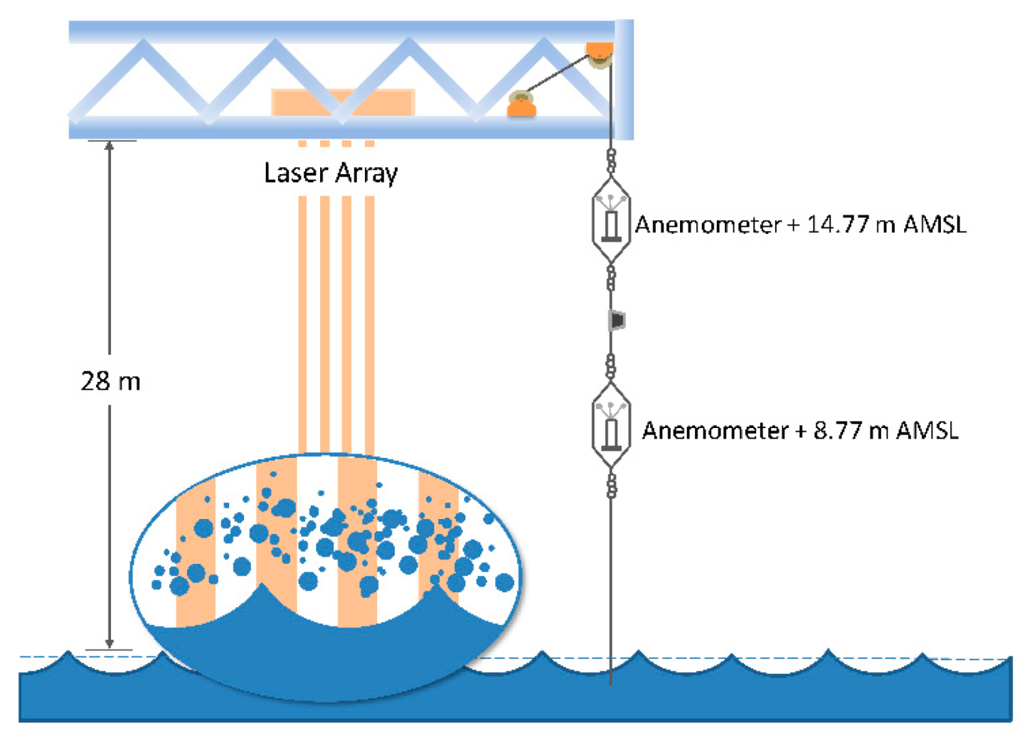
2.1. Sea Spray Volume Flux from Laser Attenuation

When a laser beam propagates through the air, its intensity decreases owing to laser radiation absorption and/or scattering along its path. Attenuation is proportional to the properties of the medium through which it travels. It is this principle that was used by Toffoli, Babanin, Donelan, Haus and Jeong [46] to determine the volume flux of sea spray in the air layer above the surface waves. That is, because each individual droplet scatters and/or absorbs laser radiation, increasing the volume of sea spray produced at the air–sea interface increases laser attenuation. Therefore, the observed laser intensity (i.e., the attenuation thereof) could be used to estimate the volume of sea spray above the ocean surface [37,46,47,48].

Formally, the relation between light intensity and attenuation can be described by the Beer–Lambert Law:

$$I\left(\mathsf{\Delta }z\right)=I_0{e}^{-\mu \mathsf{\Delta }z}$$

(1)

where $I\left(\mathsf{\Delta }z\right)$ is the attenuated laser intensity as a function of the laser propagation distance, $\mathsf{\Delta }z$; $I_0$ is the initial or reference laser intensity; and $\mu$ is the laser attenuation coefficient and depends on the properties of the medium through which it travels. Based on the laboratory measurements conducted in Air–Sea Interaction Salt-Water Tank (ASIST) of the University of Miami, Toffoli, Babanin, Donelan, Haus and Jeong [46] derived a polynomial relationship to estimate the spray volume flux from the time-averaged attenuated laser intensity directly:

$$V\left(I\right)=-3\times {10}^{-10}{I}^2+5\times {10}^{-7}I-8\times {10}^{-5}$$

(2)

where $V\left(I\right)$ is the sea spray volume flux produced per square meter of surface per second and $I$ is the averaged attenuated laser intensity in ${\mathrm{W} \mathrm{s}}^{-2}$. While Equation (2) provides the critical means to estimate the sea spray volume production in-situ, direct application in the field is hindered by its dependence on laser intensity, rather than the material property $\mu$. That is, it is not the laser intensity but the attenuation of laser intensity over the optical path length that ultimately defines the sea spray volume flux. Thus, Equation (2) needs to be reformulated in the form $V=f\left(\mu \right)$. It is here where our methodology strongly diverges from that of Toffoli, Babanin, Donelan, Haus and Jeong [46] and Ma, Babanin and Qiao [47].

To determine $V=f\left(\mu \right)$ from the experiments of Toffoli, Babanin, Donelan, Haus and Jeong [46], the initial laser intensity $I_0$ needs to be defined first (Equation (1)). As the laser intensity would be attenuated in the atmosphere even without sea spray, the base-level intensity $I_0$ is interpreted here as the laser intensity observed in the absence of wind. In Figure 1a the laser intensity variation with wind speed is shown as obtained in the laboratory experiments of Toffoli, Babanin, Donelan, Haus and Jeong [46]. We note that we corrected the wind observations of Toffoli, Babanin, Donelan, Haus and Jeong [46] following Curcic and Haus [49], and excluded the wind speed data below 20 m s⁻¹ and above 60 m s⁻¹ here as the confidence interval of these observations are relatively large (see Figure 5 in Toffoli, Babanin, Donelan, Haus and Jeong [46]). After extrapolating the laser intensity trend to $U_{10}=0$, we define the base-level laser intensity of the experiments of Toffoli, Babanin, Donelan, Haus and Jeong [46] as $I_0=1742 \mathrm{W} {\mathrm{s}}^{-2}$ (see Figure 1a) through the least-squares method (definitions of performance statistics are provided in Appendix A).

Given that the length of the optical path is defined as twice the distance between the sea surface and the measuring unit (for the laboratory experiments of Toffoli, Babanin, Donelan, Haus and Jeong [46] this corresponds to $\mathsf{\Delta }z=2.58 \mathrm{m}$), and using Equation (1), the laser attenuation coefficient $\mu$ for the experiments of Toffoli, Babanin, Donelan, Haus and Jeong [46] can be determined (see Figure 1b). By adopting a power function to define the lowest root mean square logarithmic error RMSLE of the sea spray volume flux $V\left(\mu \right)$, we obtain:

$$V\left(\mu \right)=2.80\times {10}^3·{\mu }^{6.13}$$

(3)

Thus, in any field scenario, the sea spray volume flux can now be calculated using Equations (1) and (3) if the base-level laser intensity ($I_0$), the attenuated laser intensity ($I$) and optical path ($\mathsf{\Delta }z$) are known.

2.2. Experimental Data

Wind, wave and laser intensity observations were obtained from an offshore platform located on the North-West Shelf of Western Australia, situated at a water depth of 125 m [50]. As this region is prone to tropical cyclones, measurements obtained at this platform have been used before to study wind–wave interactions during extreme weather conditions [51]. For more details on the platform and experimental setup, we refer the reader to [50,51]. In the present study, we focus on the extensive dataset that was collected from January to October of 2015.

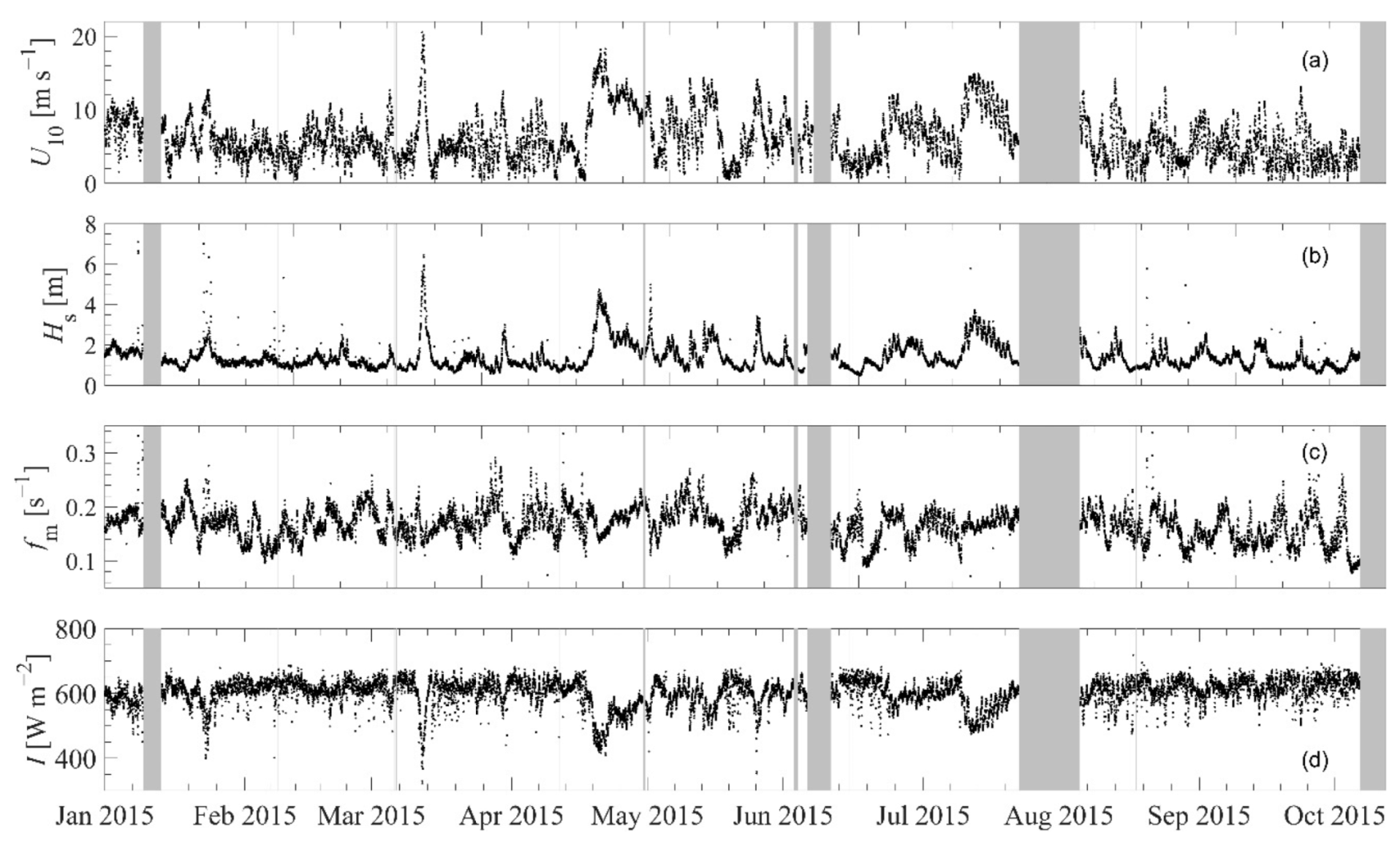
2.2.1. Wind and Wave Observations

Wind speed was measured by two ultrasonic anemometers located at 8.77 m and 14.77 m above mean sea level (MSL), respectively (Figure 2). The anemometers are fixed to a 12-mm moored wire which is kept in balance by an anchor near the seabed. The anemometers sample the three-dimensional wind speed component at a frequency of 20 Hz.

To determine the wind properties, we assume that the mean horizontal wind speed (averaged over 30-min intervals) in the marine atmospheric boundary layer is well described by a logarithmic profile:

$$U_{\mathrm{z}}\left(\mathrm{z}\right)=\frac{U_{\ast }}{\kappa }\ln \left(\frac{z}{z_0}\right)$$

(4)

where $U_{\mathrm{z}}$ is the horizontal wind speed at a distance $z$ above MSL; $U_{\ast }$ is the friction velocity; $\kappa =0.4$ is the von Kármán constant; and $z_0$ is the surface roughness length. With the wind speed measured at two locations above the sea surface, $U_{\ast }$ and $z_0$ can be obtained iteratively to estimate the wind speed at $z=10$ m reference height ($U_{10}$). Time series of $U_{10}$ from January to October 2015 are shown in Figure 3a. We note that from the 8th till the 14th of March Tropical Cyclone Olwyn passed the observation site at a distance of approximately 150–300 km [51].

The sea surface elevation was measured using four Optech Sentinel 3100 lasers positioned 28 m above MSL in a rectangular formation (1.3 m × 1.7 m) (Figure 2). This system uses a laser diode to emit short bursts of laser radiation. The emitted laser beam reflects from the ocean surface to return to the laser unit. The laser unit records the intensity of the returned beam and its propagation time. From the time of propagation optical path, and thus the position of the sea surface, can be defined.

Observations of sea surface elevation were used to determine the wave energy spectrum $F\left(f\right)$ over a period of 30 min. The spectrum was used to determine the statistical properties of the wave field, including the mean wave frequency $f_{\mathrm{m}}=\frac{{\displaystyle \int }f·F\left(f\right)df}{{\displaystyle \int }F\left(f\right)df}$ and the significant wave height, $H_{\mathrm{s}}=4\sqrt{{{\displaystyle \int }}_{f_s}^{f_{max}}F\left(f\right)df}$, where $f_s=0.8\times \frac{0.13g}{U_{10}}$ is the splitting wave frequency, which is used to separate the swell from wind waves [52], $g$ is the acceleration of gravity, and $f_{max}$ is the upper-frequency limit of the spectrum. We choose to remove swell contributions from the statistical representation of the wave properties, as wind waves are expected to dominate sea spray production as swell waves are less likely to break due to their smaller steepness. Timeseries of the significant wave height of wind waves and the mean wave frequency from January to October in 2015 are shown in Figure 3b,c, respectively.

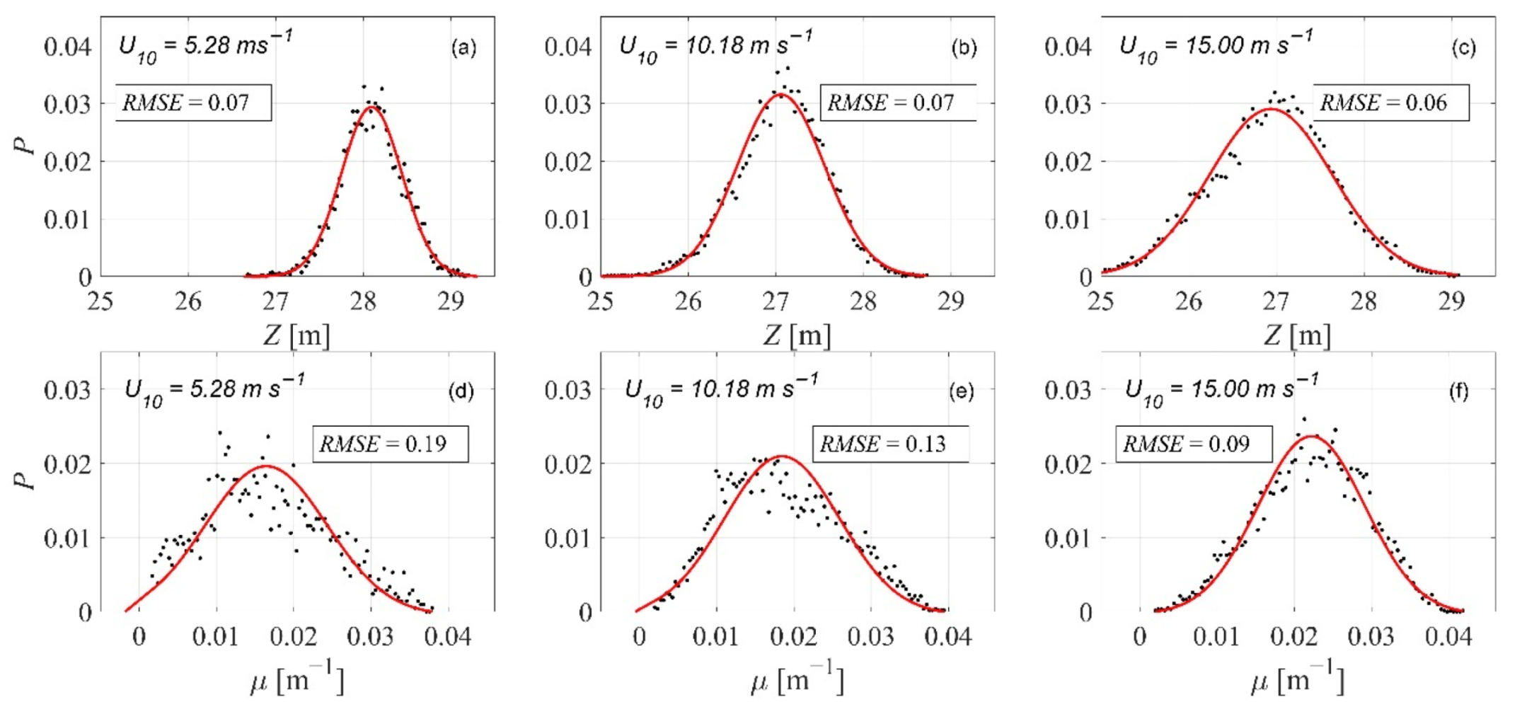
2.2.2. Laser Intensity

The attenuated laser intensity ($I$) was measured simultaneously with the sea surface elevation and examples of its distribution for three different wind speeds are shown in Figure 4. The probability density distribution of the attenuated laser intensity typically consists of three modes. The first mode of the measured laser intensity ranges from $0$ to $200 {\mathrm{W} \mathrm{s}}^{-2}$ and is typically much lower than its mean due to the partial dropout of the returning laser radiation, that is, fewer than 50% of laser shots return to the laser unit. The third mode of the laser intensity covers a high-intensity range from about $1000$ to $2000{ \mathrm{W} \mathrm{s}}^{-2}$ and is caused by a laser saturation error. In this mode, the reflection of the laser beam from the sea surface is too strong (i.e., the laser works best on a diffusive surface), thereby contaminating the observed intensity of the reflected laser beam. We note that, hereafter, only laser intensity observations from the second mode are considered.

3. Results

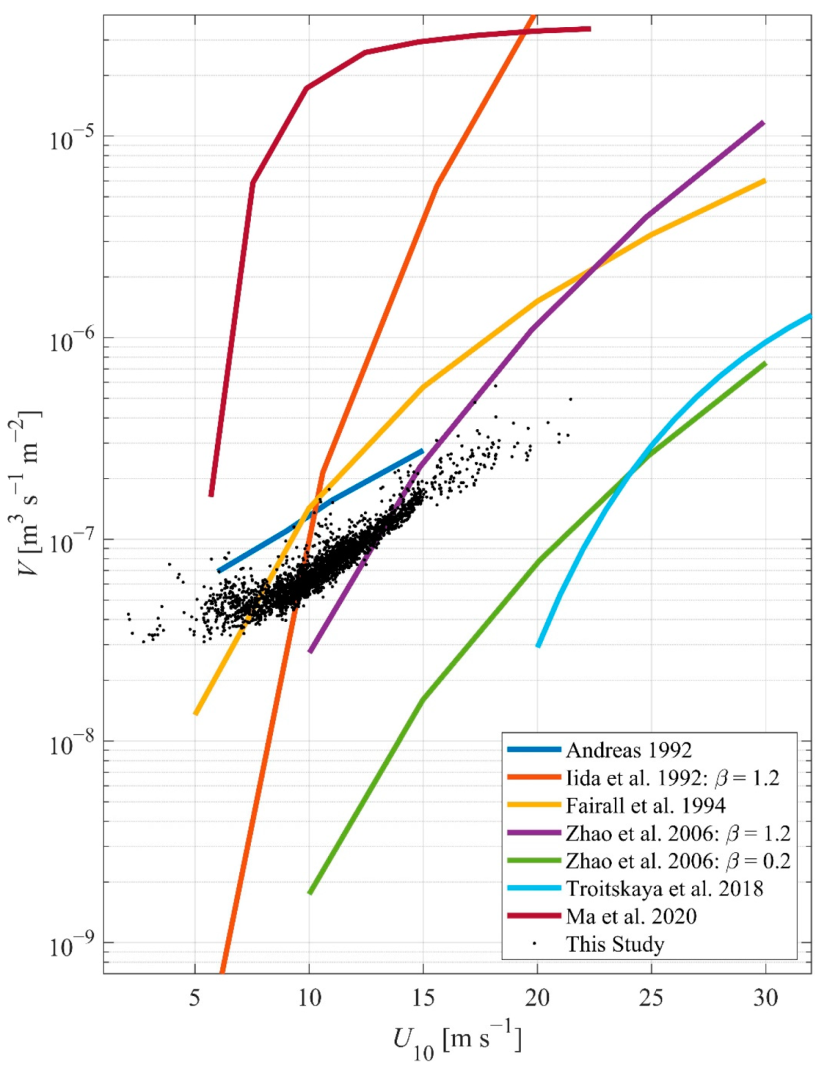
3.1. Sea Spray Volume Flux

Before Equation (3) can be applied to estimate the sea spray volume flux from the laser intensity observations, the base-level intensity $I_0$ needs to be determined for the field experimental setup. Figure 5 shows the probability density function of the laser intensity observations over the complete period from January to October 2015. The base-level laser intensity was determined by extrapolating the probability density distribution of the attenuated laser intensity to 0, yielding $I_0=1400 {\mathrm{W} \mathrm{s}}^{-2}$.

As the removal of the first and third mode from the laser intensity record can unwantedly impact the accuracy of the data, a quality control procedure is applied to the laser attenuation observations before they are used to estimate sea spray volume flux. We first discard any observations where more than 50% of the record is removed. While the removal of half the timeseries is large, we confirm that there is no correlation between the removed data and the phase of the measured surface elevation and thus no bias is expected in the measured laser intensity after the removal. To reduce the impact of data removal on the accuracy of the observations, we fit a Gaussian distribution to the distribution of the laser attenuation timeseries and dismiss any data where the RMSE $\ge 0.13$ (given 100 interval bins). This value was chosen as a trade-off between the volume of discarded data and the scatter of the probability density distribution of $\mu$. Similar to an example of the distribution of sea surface elevation (Figure 6a–c), Figure 6d,e provides an example of the distributions of $\mu$ where $\mathrm{RMSE}\le 0.19$. With $I_0$ being $1400 {\mathrm{W} \mathrm{s}}^{-2}$ and $\mathsf{\Delta }z$ being twice the distance between laser source and the instantaneous sea surface, the mean laser attenuation coefficient can then be determined through Equation (1). Figure 7 illustrates the variation of attenuation coefficient with wind speed prior to and following the quality control.

Given that $\mu$ is now known, the sea spray volume flux can be estimated using Equation (3) (Figure 8). Our observations of the sea spray volume flux increase steadily with wind speed and are well within the ranges of existing sea spray volume flux parameterizations. Notably, our observations are consistent with the model proposed by Andreas [6] in both trend and magnitude. Although extrapolation of our observations to higher wind speeds comes with great uncertainties, the rate of increase with wind speed would correspond well to the models of Fairall, Kepert and Holland [4], Zhao, Toba, Sugioka and Komori [42] and Troitskaya, Kandaurov, Ermakova, Kozlov, Sergeev and Zilitinkevich [26].

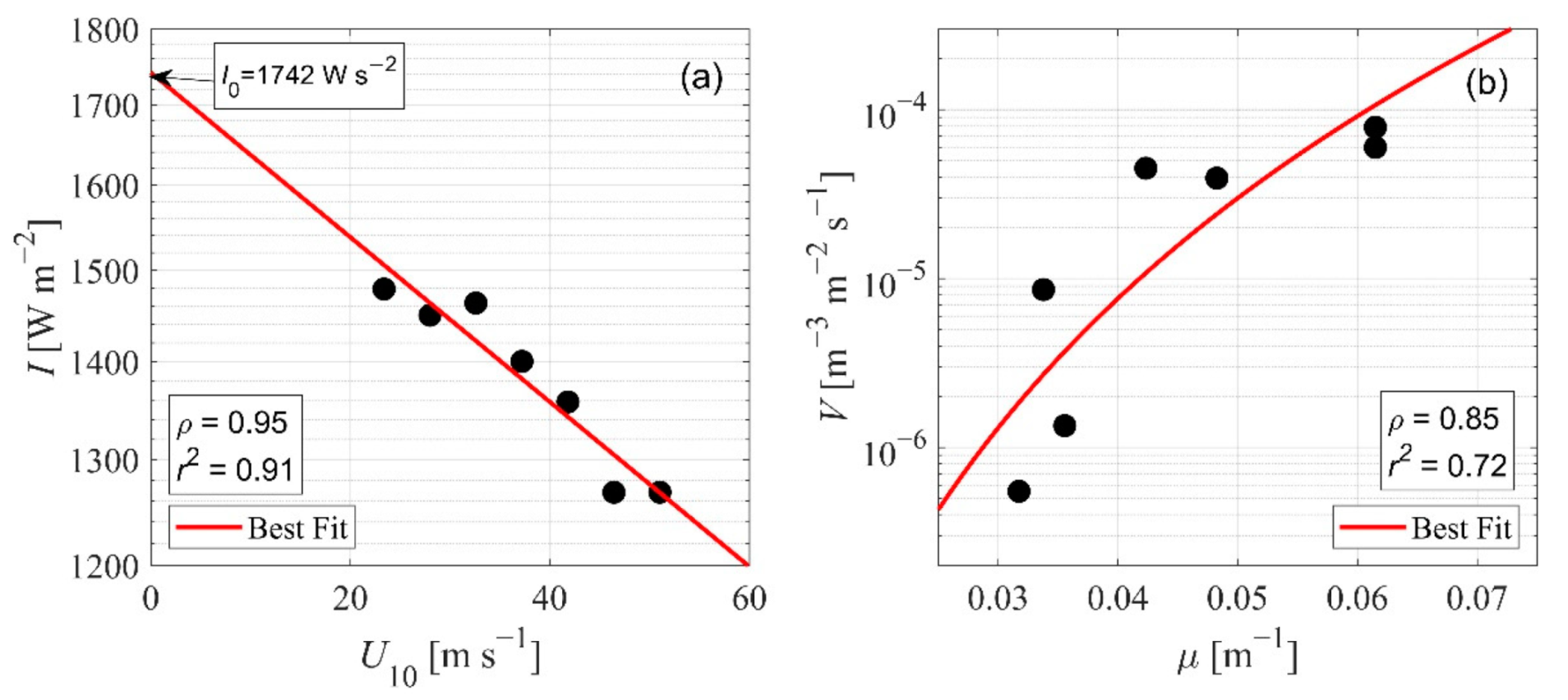
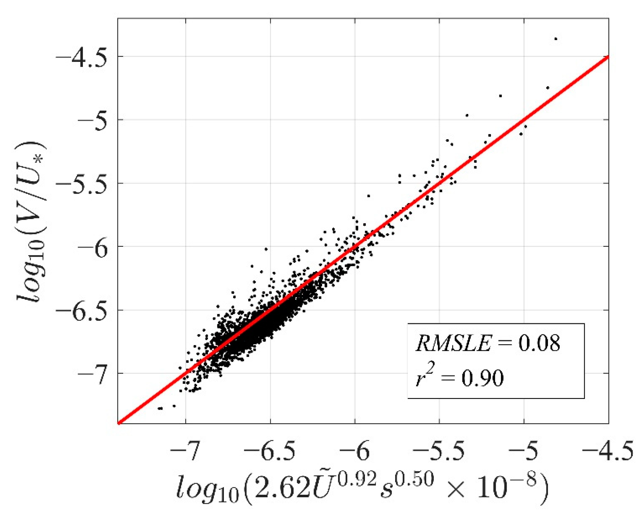
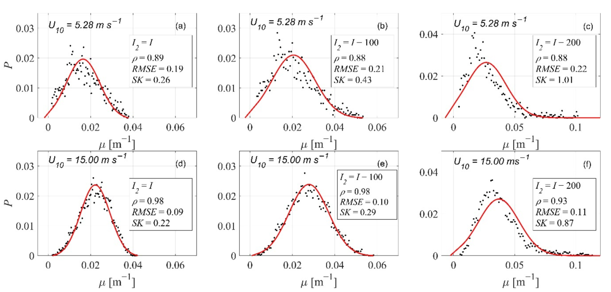
3.2. Sea Spray Volume Flux Parameterization

Using the field observations of the sea spray volume flux, a sea spray volume flux model can be constructed. As sea spray droplets are generated at the ocean surface through the processes of wave breaking and wind shear, the sea spray volume flux is expected to be determined by the properties of the surface roughness length, local wind, and wave field.

$$V=f\left(\mathrm{wind},\mathrm{wave}\right).$$

(5)

For dimensional consistency, non-dimensional parameters were adopted to construct the model. As the wind stress fundamentally defines the resistance of the ocean surface to the wind, and thus the capacity of wind to tear of droplets from the wave crests, the friction velocity is used to normalize the wind speed, i.e., $\tilde{U}=\frac{U_{10}}{U_{\ast }}$. To include the effects of breaking waves, the mean wave steepness, $s=\frac{H_{\mathrm{s}}{k}_m}{2}$ is used here as a proxy of wave breaking severity, where $k_m$ is the mean wavenumber. In line with $\tilde{U}$, the sea spray volume flux, which ultimately has the dimensions of ${\mathrm{m} \mathrm{s}}^{-1}$, is also scaled by the shear velocity $\tilde{V}=\frac{V\left(\mu \right)}{U_{\ast }}$, as $U_{\ast }$ includes both effects of wind and waves. We note that this scaling via $U_{\ast }$ is commonly adopted by others as well. For instance, Emanuel [54] provided a scaling parameter functioned by $U_{\ast }$ on the basis of a scale analysis of spray, and later adopted by Fairall, Banner, Peirson, Asher and Morison [29]. Additionally, both Lenain and Melville [37] and Zhao, Toba, Sugioka and Komori [42] scaled the production of sea spray using parameters defined by $U_{\ast }$. A simple power-law model is used to parameterize the sea spray volume flux:

$$\tilde{V}=a{\tilde{U}}^b{s}^c.$$

(6)

The best-fit relation, based on the lowest RMSLE, is shown in Figure 9, and is given by $a=2.62\times {10}^{-8}$, $b=0.92$, and $c=0.50$ with $RMSLE=0.08$ and $r^2=0.90$. Therefore, the wind–wave-dependent sea spray flux model is:

$$\tilde{V}=2.62{\tilde{U}}^{0.92}{s}^{0.50}\times {10}^{-8}.$$

(7)

Taking into consideration that Equation (7) is an empirical fit rather than a complete physical construct, we hypothesize that the volume flux varies linearly with the non-dimensional wind speed and as the square of the mean wave steepness. In that case, Equation (7) reduces to the form:

$$\frac{V}{U_{10}}=1.99\sqrt{s}\times {10}^{-8}$$

(8)

where $a=1.99\times {10}^{-8}$, $b=1.00$, and with $RMSLE=0.09$ and $r^2=0.89$. In addition, to further identify the role of wave properties in the production of sea spray, we eliminate the $\sqrt{s}$ term from Equation (8) and then refit $\tilde{V}$ by $\tilde{U}$ alone based on the lowest RMSLE to determine the relation between spray production and wind alone. We note, however, that this still implicitly includes wave effects through $U_{\ast }$. This then results in $a=1.15\times {10}^{-8}, b=0.87$, with $RMSLE=0.10$ and $r^2=0.87$. The increase in RMSLE and decrease in $r^2$ with respect to Equation (7) thus suggesting that the inclusion of wave properties through the mean wave steepness improves the spray volume flux parameterization. This is highly consistent with recent studies indicating that it is necessary to incorporate wave properties into sea spray models, rather than using wind properties alone to parameterize the sea spray production [37,41,42,43,44,45].

4. Discussion

In this study, we presented rare in-situ observations of the ocean sea spray flux under a wide range of wind and wave conditions using laser altimeters. We did so by adopting the principles of the Beer–Lambert Law, stating that as the laser beam propagates through the atmosphere laden with sea spray, the droplets largely scatter and/or absorb part of the laser radiation to attenuate and dominant the variation of intensity of the laser beam. While this conceptual idea of estimating spray volume flux using the laser intensity attenuation rate was used to estimate the sea spray flux in the innovative laboratory and field studies of Toffoli, Babanin, Donelan, Haus and Jeong [46] and Ma, Babanin and Qiao [47], the fundamental principle of the Beer–Lambert Law was not considered. We therefore extended the methodologies used by Toffoli, Babanin, Donelan, Haus and Jeong [46] and Ma, Babanin and Qiao [47] to obtain estimates of the ocean sea spray flux in situ and developed a sea spray flux parameterization covering, for the very first time, a wide range of wind and wave conditions.

Some caution is, however, required in interpreting the laser attenuation rate as a proxy of the sea spray volume flux. Strictly speaking, it is the sea spray volume, and not its flux, which attenuates the laser intensity and one can only determine the sea spray volume flux from the observed laser attenuation rate if the total volume of sea spray droplets diffused upwards into the atmospheric boundary layer is small compared to the volume of droplets that re-enter the ocean rapidly. This is, for instance, the case in the experiments of Toffoli, Babanin, Donelan, Haus and Jeong [46] where the optical path length $\mathsf{\Delta }z$ is relatively small. To validate that we did not erroneously overestimate $V$ by ignoring those droplets that were airborne for significant periods of time, we consider the laser attenuation probability density function of a 5 m s⁻¹ and 15 m s⁻¹ wind speed event (Figure 10a,d). Here, we assume a priori that the amount of suspended sea spray is negligible. We mimic the presence of background sea spray by reducing the observed laser intensity uniformly in time which leads to a positively skewed distribution of the laser attenuation (Figure 10b,c,e,f) as opposed to the Gaussian distributions we observe (Figure 6). As such, if a considerable volume of suspended sea spray droplets would indeed be present, the quality control procedure described in Section 3.1 would likely have removed the event from the dataset. We note that the impact of added background sea spray on the skewness of the laser attenuation distribution is most apparent for the low wind speed case. It is perhaps for this reason that the sea spray volume flux prior to quality control is relatively large (see Figure 7) as under these conditions the sea spray volume between the laser and the ocean is dominated by the suspended droplets rather than those droplets instantaneously produced at the sea surface. Lastly, as previously substantiated by studies at severe winds [6,42], spume droplets account for the majority of the total volumetric concentration of spray in the air [42]. To be more precise, when the volume fraction of spume droplets is addressed in contemporary sea spray models [1,6,14,55], spume dominates more than $95\%$ of the overall volumetric concentration of the spray for $U_{10}=10-15{ \mathrm{m} \mathrm{s}}^{-1}$. This is not only because individual spume droplets have a larger radius, thus containing significantly more water, but also because the quantity of spume droplets formed is substantial [26,38]. As such, the impact of suspended sea spray droplets on our estimation of the sea spray volume flux is expected to be modest. However, when wind speeds are low, resulting in a near-absence of spume droplets, we expect that suspended droplets cannot be ignored. Targeted control experiments are required to elucidate the environmental restrictions on the methodologies utilized in this investigation, particularly the impacts of suspended droplets at low winds and the physical sea surface roughness on laser backscatter modulation. Opportunities to derive the droplet size distribution from laser altimeters should be explored to improve the further potential of the methods proposed in this study and allow a more detailed comparison against existing physical and theoretical models.

While sea spray can critically contribute to the heat exchange between the atmosphere and ocean, its physics are often not considered in contemporary air–sea flux prediction models, such as the popular COARE 2.6 bulk flux algorithm [13,56,57]. The foremost reason that sea spray is not considered is the significant uncertainty of current sea spray volume flux models which is mostly caused by the lack of in-situ observational data to validate against. To circumvent such limitations, studies tend to interpret sea spray model performance by validating the coupled air–sea models instead through much more readily available and measurable properties, such as wind speed and wave height [9,56,57,58,59]. Here, however, we developed a sea spray volume flux model based on uniquely in-situ observations of sea spray. Promisingly, our observations are consistent with the spray model of Andreas [6] in both magnitude and trend.

Considering the coincidence between our observations and the model of Andreas [6], our results indirectly substantiate the critical importance of sea spray on the dynamics of extreme marine weather events. For example, Zhao, Qiao, Cavaleri, Wang, Bertotti and Liu [58], through implementing the spray model of Andreas [6] into FIO-AOW system, suggested that the sea spray enhances heat transfer at sea surface and leads to a substantial increase in wind velocity especially in the areas surrounding the TC eye [58]. Moreover, Garg, Ng and Narasimalu [59] included sea spray induced heat flux into the air–sea numerical module in the WRF-MIKE3-MIKE 21 SW coupled model and stated that when considering the spray-mediated heat flux there would be a reduction in the sensible heat flux, increase in the storm intensity and broadening of the storm core [59]. Thus, our results tend to imply, albeit indirectly, that sea spray has indeed a positive feedback on storm intensification and assists in sustaining tropical cyclones [12,13].

Previous studies have stressed the need to incorporate wave properties in sea spray production parameterizations as sea spray is ultimately generated through the interactions between wind and waves [43,44,58]. In their spray and/or aerosol models, wave age is considered as the dominant wave parameter to characterize the sea state (noting that the wind–wave Reynolds number can be interpreted as the product of the wind stress and wave age). However, while important, wave age alone cannot fully capture the properties of the sea state as it provides information on the relative speed of the most energetic wave with respect to the wind only. In this study, we observe that the wave steepness provides a better proxy to our dataset in contrast to the wave age. Given that wave steepness is a critical parameter in the quantification of wave breaking, our observations signify the importance of wave breaking in the generation of sea spray. In addition, even though our observations and our model are consistent with the sea spray volume flux model of Andreas [6], it is here where our model is distinctly different from Andreas [6] which, unlike our model, does not depend explicitly on the properties of the wave field. In addition, as our observations are restricted to 22 m s⁻¹ only, it remains open how our parameterization performs for higher wind speeds as the physical processes that drive wind–wave interactions are expected to change at a wind speed of about 29 m s⁻¹ [49,60]. Therefore, more in-situ observations during extreme marine weather conditions are required to determine the dependence of sea spray generation on both wind and wave properties, while further numerical studies are required to determine how our wave steepness depended on model impacts storm dynamics as opposed to sea spray models relying on wind properties alone.

5. Conclusions

We presented a large and novel dataset of in-situ sea spray observations obtained under a wide range of wind and wave field conditions. Using the Beer–Lambert law we expanded the methodologies adopted by Toffoli, Babanin, Donelan, Haus and Jeong [46] and Ma, Babanin and Qiao [47] to estimate the sea spray volume flux from laser intensity observations. Sea spray observations are used to develop a nondimensional wind–wave-dependent sea spray volume flux model $V/U_{\ast }=2.62{\left(\frac{U_{10}}{U_{\ast }}\right)}^{0.92}{s}^{0.50}\times {10}^{-8}$, or the approximation thereof $V/U_{10}=1.99\sqrt{s}\times {10}^{-8}$, where $V$, $U_{10}$, and are the spray volume flux, 10-m wind speed and wind speed, respectively, and $s$ is the mean wave steepness. We find that our observations and the derived spray model correspond well to the sea spray model of Andreas [6]. Based on previous studies that adopted the spray model of Andreas [6], our observations indirectly substantiate the importance of sea spray in enhancing the air–sea heat and moisture exchange, and storm intensification. In addition, as our observations of the sea spray volume flux are limited to wind speeds up to 22 m s⁻¹, more observations of sea spray are needed to understand the impact of waves on sea spray generation during extreme marine weather conditions.

References

1. Veron, F. Ocean spray. Annu. Rev. Fluid Mech. 2015, 47, 507–538. [Google Scholar] [CrossRef]
2. Wu, L.; Cheng, X.; Zeng, Q.; Jin, J.; Huang, J.; Feng, Y. On the upward flux of sea-spray spume droplets in high-wind conditions. J. Geophys. Res. Atmos. 2017, 122, 5976–5987. [Google Scholar] [CrossRef]
3. Edson, J.B.; Andreas, E.L. Modeling the role of sea spray on air-sea heat and moisture exchange. Final Rep. 1997, 6, 18. [Google Scholar]
4. Fairall, C.; Kepert, J.; Holland, G. The effect of sea spray on surface energy transports over the ocean. Global Atmos. Ocean Syst. 1994, 2, 121–142. [Google Scholar]
5. Van Eijk, A.; Kusmierczyk-Michulec, J.; Francius, M.; Tedeschi, G.; Piazzola, J.; Merritt, D.; Fontana, J. Sea-spray aerosol particles generated in the surf zone. J. Geophys. Res. Atmos. 2011, 116, 29397–29409. [Google Scholar] [CrossRef] [Green Version]
6. Andreas, E.L. Sea spray and the turbulent air-sea heat fluxes. J. Geophys. Res. Oceans 1992, 97, 11429–11441. [Google Scholar] [CrossRef]
7. Andreas, E.L. Spray stress revisited. J. Phys. Oceanogr. 2004, 34, 1429–1440. [Google Scholar] [CrossRef]
8. Powell, M.D.; Vickery, P.J.; Reinhold, T.A. Reduced drag coefficient for high wind speeds in tropical cyclones. Nature 2003, 422, 279–283. [Google Scholar] [CrossRef]
9. Liu, B.; Liu, H.; Xie, L.; Guan, C.; Zhao, D. A coupled atmosphere–wave–ocean modeling system: Simulation of the intensity of an idealized tropical cyclone. Mon. Weather Rev. 2011, 139, 132–152. [Google Scholar] [CrossRef]
10. Donelan, M.A.; Haus, B.K.; Reul, N.; Plant, W.J.; Stiassnie, M.; Graber, H.C.; Brown, O.B.; Saltzman, E.S. On the limiting aerodynamic roughness of the ocean in very strong winds. Geophys. Res. Lett. 2004, 31, L18306. [Google Scholar] [CrossRef] [Green Version]
11. Veron, F.; Hopkins, C.; Harrison, E.L.; Mueller, J.A. Sea spray spume droplet production in high wind speeds. Geophys. Res. Lett. 2012, 39, L16602. [Google Scholar] [CrossRef] [Green Version]
12. Andreas, E.L.; Emanuel, K.A. Effects of sea spray on tropical cyclone intensity. J. Atmos. Sci. 2001, 58, 3741–3751. [Google Scholar] [CrossRef] [Green Version]
13. Andreas, E.L.; Persson, P.O.G.; Hare, J.E. A bulk turbulent air–sea flux algorithm for high-wind, spray conditions. J. Phys. Oceanogr. 2008, 38, 1581–1596. [Google Scholar] [CrossRef]
14. Andreas, E.L. A new sea spray generation function for wind speeds up to 32 ms−1. J. Phys. Oceanogr. 1998, 28, 2175–2184. [Google Scholar] [CrossRef] [Green Version]
15. De Leeuw, G.; Andreas, E.L.; Anguelova, M.D.; Fairall, C.; Lewis, E.R.; O’Dowd, C.; Schulz, M.; Schwartz, S.E. Production flux of sea spray aerosol. Rev. Geophys. 2011, 49, RG2001. [Google Scholar] [CrossRef] [Green Version]
16. Thorpe, S. Bubble clouds and the dynamics of the upper ocean. Q. J. R. Meteorol. Soc. 1992, 118, 1–22. [Google Scholar] [CrossRef]
17. Melville, W.K. The role of surface-wave breaking in air-sea interaction. Annu. Rev. Fluid Mech. 1996, 28, 279–321. [Google Scholar] [CrossRef]
18. Spiel, D.E. More on the births of jet drops from bubbles bursting on seawater surfaces. J. Geophys. Res. Oceans 1997, 102, 5815–5821. [Google Scholar] [CrossRef]
19. Resch, F.; Afeti, G. Film drop distributions from bubbles bursting in seawater. J. Geophys. Res. Oceans 1991, 96, 10681–10688. [Google Scholar] [CrossRef]
20. Lhuissier, H.; Villermaux, E. Bursting bubble aerosols. J. Fluid Mech. 2012, 696, 5. [Google Scholar] [CrossRef] [Green Version]
21. MacIntyre, F. Flow patterns in breaking bubbles. J. Geophys. Res. 1972, 77, 5211–5228. [Google Scholar] [CrossRef]
22. Andreas, E. Andreas, E. A review of spray generation function for the open ocean. In Atmosphere-Ocean Interactions Volume 1; Perrie, W., Ed.; WIT Press: Billerica, MA, USA, 2002; pp. 1–46. [Google Scholar]
23. Andreas, E.L.; Edson, J.B.; Monahan, E.C.; Rouault, M.P.; Smith, S.D. The spray contribution to net evaporation from the sea: A review of recent progress. Bound. Layer Meteorol. 1995, 72, 3–52. [Google Scholar] [CrossRef]
24. Koga, M. Direct production of droplets from breaking wind-waves—Its observation by a multi-colored overlapping exposure photographing technique. Tellus 1981, 33, 552–563. [Google Scholar] [CrossRef] [Green Version]
25. Monahan, E.C. Sea spray as a function of low elevation wind speed. J. Geophys. Res. 1968, 73, 1127–1137. [Google Scholar] [CrossRef]
26. Troitskaya, Y.; Kandaurov, A.; Ermakova, O.; Kozlov, D.; Sergeev, D.; Zilitinkevich, S. The “bag breakup” spume droplet generation mechanism at high winds. Part I: Spray generation function. J. Phys. Oceanogr. 2018, 48, 2167–2188. [Google Scholar] [CrossRef]
27. Monahan, E.C.; Davidson, K.L.; Spiel, D.E. Whitecap aerosol productivity deduced from simulation tank measurements. J. Geophys. Res. Oceans 1982, 87, 8898–8904. [Google Scholar] [CrossRef]
28. Andreas, E.L. Parameterizing scalar transfer over snow and ice: A review. J. Hydrometeorol. 2002, 3, 417–432. [Google Scholar] [CrossRef]
29. Fairall, C.; Banner, M.; Peirson, W.; Asher, W.; Morison, R. Investigation of the physical scaling of sea spray spume droplet production. J. Geophys. Res. Oceans 2009, 114, C10001. [Google Scholar] [CrossRef]
30. Hultin, K.A.H.; Nilsson, E.D.; Krejci, R.; Mårtensson, E.M.; Ehn, M.; Hagström, Å.; de Leeuw, G. In situ laboratory sea spray production during the marine aerosol production 2006 cruise on the northeastern atlantic ocean. J. Geophys. Res. Atmos. 2010, 115, D062012. [Google Scholar] [CrossRef]
31. Norris, S.J.; Brooks, I.M.; Hill, M.K.; Brooks, B.J.; Smith, M.H.; Sproson, D.A.J. Eddy covariance measurements of the sea spray aerosol flux over the open ocean. J. Geophys. Res. Atmos. 2012, 117, D07210. [Google Scholar] [CrossRef]
32. Hartery, S.; Toohey, D.; Revell, L.; Sellegri, K.; Kuma, P.; Harvey, M.; McDonald, A.J. Constraining the surface flux of sea spray particles from the southern ocean. J. Geophys. Res. Atmos. 2020, 125, D032026. [Google Scholar] [CrossRef]
33. Ozeki, T.; Toda, S.; Yamaguchi, H. Field investigation of impinging seawater spray on the R/V mirai using spray particle counter type sea spray meter. In Proceedings of the 33rd International Symposium on Okhotsk Sea and Polar Oceans, Hokkaido, Japan, 18–21 February 2018; pp. 93–96. [Google Scholar]
34. Engelmann, R.; Kanitz, T.; Baars, H.; Heese, B.; Althausen, D.; Skupin, A.; Wandinger, U.; Komppula, M.; Stachlewska, I.S.; Amiridis, V. The automated multiwavelength Raman polarization and water-vapor lidar Polly XT: The neXT generation. Atmos. Meas. Tech. 2016, 9, 1767–1784. [Google Scholar] [CrossRef] [Green Version]
35. Dhar, S.; Khawaja, H.A. Recognizing potential of LiDAR for comprehensive measurement of sea spray flux for improving the prediction of marine icing in cold conditions—A review. Ocean Eng. 2021, 223, 108668. [Google Scholar] [CrossRef]
36. Smith, M.; Park, P.; Consterdine, I. Marine aerosol concentrations and estimated fluxes over the sea. Q. J. R. Meteorol. Soc. 1993, 119, 809–824. [Google Scholar] [CrossRef]
37. Lenain, L.; Melville, W.K. Evidence of sea-state dependence of aerosol concentration in the marine atmospheric boundary layer. J. Phys. Oceanogr. 2017, 47, 69–84. [Google Scholar] [CrossRef]
38. Mehta, S.; Ortiz-Suslow, D.G.; Smith, A.W.; Haus, B.K. A Laboratory investigation of spume generation in high winds for fresh and seawater. J. Geophys. Res. Atmos. 2019, 124, 11297–11312. [Google Scholar] [CrossRef]
39. Ortiz-Suslow, D.G.; Haus, B.K.; Mehta, S.; Laxague, N.J.M. Sea spray generation in very high winds. J. Atmos. Sci. 2016, 73, 3975–3995. [Google Scholar] [CrossRef]
40. Nilsson, E.D.; Hultin, K.A.H.; Mårtensson, E.M.; Markuszewski, P.; Rosman, K.; Krejci, R. Baltic sea spray emissions: In situ eddy covariance fluxes vs. simulated tank sea spray. Atmosphere 2021, 12, 274. [Google Scholar] [CrossRef]
41. Zhao, D.; Toba, Y. Dependence of whitecap coverage on wind and wind-wave properties. J. Oceanogr. 2001, 57, 603–616. [Google Scholar] [CrossRef]
42. Zhao, D.; Toba, Y.; Sugioka, K.-i.; Komori, S. New sea spray generation function for spume droplets. J. Geophys. Res. 2006, 111, C02007. [Google Scholar] [CrossRef]
43. Norris, S.J.; Brooks, I.M.; Salisbury, D.J. A wave roughness Reynolds number parameterization of the sea spray source flux. Geophys. Res. Lett. 2013, 40, 4415–4419. [Google Scholar] [CrossRef] [Green Version]
44. Ovadnevaite, J.; Manders, A.; De Leeuw, G.; Ceburnis, D.; Monahan, C.; Partanen, A.-I.; Korhonen, H.; O’Dowd, C. A sea spray aerosol flux parameterization encapsulating wave state. Atmos. Chem. Phys. 2014, 14, 1837–1852. [Google Scholar] [CrossRef] [Green Version]
45. Laussac, S.; Piazzola, J.; Tedeschi, G.; Yohia, C.; Canepa, E.; Rizza, U.; Van Eijk, A.M.J. Development of a fetch dependent sea-spray source function using aerosol concentration measurements in the north-western mediterranean. Atmos. Environ. 2018, 193, 177–189. [Google Scholar] [CrossRef]
46. Toffoli, A.; Babanin, A.V.; Donelan, M.A.; Haus, B.K.; Jeong, D. Estimating sea spray volume with a laser altimeter. J. Atmos. Ocean. Technol. 2011, 28, 1177–1183. [Google Scholar] [CrossRef]
47. Ma, H.; Babanin, A.V.; Qiao, F. Field observations of sea spray under Tropical Cyclone Olwyn. Ocean Dyn. 2020, 70, 1439–1448. [Google Scholar] [CrossRef]
48. Fairall, C.; Pezoa, S.; Moran, K.; Wolfe, D. An observation of sea-spray microphysics by airborne doppler radar. Geophys. Res. Lett. 2014, 41, 3658–3665. [Google Scholar] [CrossRef]
49. Curcic, M.; Haus, B.K. Revised Estimates of ocean surface drag in strong winds. Geophys. Res. Lett. 2020, 47, e2020GL087647. [Google Scholar] [CrossRef]
50. Babanin, A.V.; Wake, G.G.; McConochie, J. Field observation site for air-sea interactions in tropical cyclones. In Proceedings of the International Conference on Offshore Mechanics and Arctic Engineering, Busan, Korea, 18 October 2016; p. V003T002A002. [Google Scholar]
51. Voermans, J.J.; Rapizo, H.; Ma, H.; Qiao, F.; Babanin, A.V. Air–sea momentum fluxes during tropical cyclone olwyn. J. Phys. Oceanogr. 2019, 49, 1369–1379. [Google Scholar] [CrossRef]
52. Portilla, J.; Ocampo-Torres, F.J.; Monbaliu, J. Spectral partitioning and identification of wind sea and swell. J. Atmos. Ocean. Technol. 2009, 26, 107–122. [Google Scholar] [CrossRef]
53. Iida, N.; Toba, Y.; Chaen, M. A new expression for the production rate of sea water droplets on the sea surface. J. Oceanogr. 1992, 48, 439–460. [Google Scholar] [CrossRef]
54. Emanuel, K. A similarity hypothesis for air–sea exchange at extreme wind speeds. J. Atmos. Sci. 2003, 60, 1420–1428. [Google Scholar] [CrossRef]
55. Monahan, E.C.; Staniec, A.; Vlahos, P. Spume drops: Their potential role in air-sea gas exchange. J. Geophys. Res. Oceans 2017, 122, 9500–9517. [Google Scholar] [CrossRef]
56. Zhang, L.; Zhang, X.; Perrie, W.; Guan, C.; Dan, B.; Sun, C.; Wu, X.; Liu, K.; Li, D. Impact of sea spray and sea surface roughness on the upper ocean response to super typhoon haitang. J. Phys. Oceanogr. 2021, 51, 1929–1945. [Google Scholar]
57. Zhang, L.; Zhang, X.; Chu, P.C.; Guan, C.; Fu, H.; Chao, G.; Han, G.; Li, W. Impact of sea spray on the yellow and east China seas thermal structure during the passage of typhoon rammasun. J. Geophys. Res. Oceans 2017, 122, 7783–7802. [Google Scholar] [CrossRef] [Green Version]
58. Zhao, B.; Qiao, F.; Cavaleri, L.; Wang, G.; Bertotti, L.; Liu, L. Sensitivity of typhoon modeling to surface waves and rainfall. J. Geophys. Res. Oceans 2017, 122, 1702–1723. [Google Scholar] [CrossRef]
59. Garg, N.; Ng, E.Y.K.; Narasimalu, S. The effects of sea spray and atmosphere–wave coupling on air–sea exchange during a tropical cyclone. Atmos. Chem. Phys. 2018, 18, 6001–6021. [Google Scholar] [CrossRef] [Green Version]
60. Babanin, A.V.; Rogers, W.E.; de Camargo, R.; Doble, M.; Durrant, T.; Filchuk, K.; Ewans, K.; Hemer, M.; Janssen, T.; Kelly-Gerreyn, B.; et al. Waves and Swells in High Wind and Extreme Fetches, Measurements in the Southern Ocean. Front. Mar. Sci. 2019, 6, 361. [Google Scholar] [CrossRef] [Green Version]
Figure 1. The recalibration of laboratory observations of Toffoli, Babanin, Donelan, Haus and Jeong [46]: (a) the attenuated laser intensity I against wind speed U 10 and (b) the sea spray volume flux V against the laser attenuation coefficient μ . The red line defines the best data fit based on the power law.
Jmse 09 01168 g001
Figure 2. Configuration of the observation platform and instruments. The rectangular laser array is attached to the flare bridge 28 m above MSL. Two anemometers are fixed at 8.77 m and 14.77 m above the MSL, respectively.
Jmse 09 01168 g002
Figure 3. Timeseries of wind and wave properties over 30 min periods: (a) The mean wind speed at 10 m reference height, U 10 (b) The significant wave height of wind waves, H s . (c) The mean wave frequency, f m . (d) The attenuated laser intensity of the second laser intensity mode, I . Periods where data are unavailable are highlighted in grey.
Jmse 09 01168 g003
Figure 4. (a) An example of the probability density distribution of the attenuated laser intensity I for a 5 m s−1 wind speed event. (b,c) Same as (a) but for a 10 m s−1 and 15 m s−1 wind speed event, respectively.
Jmse 09 01168 g004
Figure 5. The probability density distribution of the attenuated laser intensity with initial laser intensity, I 0 = 1400   W   s 2 , from January to October in 2015.
Jmse 09 01168 g005
Figure 6. Examples of the probability density distribution of the laser range, Z, (ac), and the laser intensity attenuation coefficient, μ (df) under various wind conditions. Red solid lines are Gaussian regression fitting to experimental samples for a 5 m s−1, 10 m s−1 and 15 m s−1 wind speed event, respectively. The root mean square error RMSE was utilized to evaluate the performance of the fitting.
Jmse 09 01168 g006
Figure 7. The attenuation coefficient varies with U 10 . Grey dots are the laser intensity attenuation coefficient with systemic error. Black dots are the laser intensity attenuation coefficient after quality control.
Jmse 09 01168 g007
Figure 8. Comparison of the estimated sea spray volume flux from field observations in this study (black dots) with parametrizations of: Andreas [6], the blue line; Iida, et al. [53] with wave age of 1.2, the orange line; Fairall, Kepert and Holland [4] with, the yellow line; Zhao, Toba, Sugioka and Komori [42] with wave age of 1.2 and 0.2, the purple line and green line, respectively; Troitskaya, Kandaurov, Ermakova, Kozlov, Sergeev and Zilitinkevich [26], the light blue line; Ma, Babanin and Qiao [47], the red solid line.
Jmse 09 01168 g008
Figure 9. Logarithm-scale plot of dimensionless sea spray volume flux of the measurement versus wind–wave-dependent model (Equation (7)). The solid red line is 1:1 line.
Jmse 09 01168 g009
Figure 10. (a) An example of the probability density distribution of the laser attenuation coefficient for a 5 m s−1 wind speed event. Red solid line is Gaussian regression fitting to experimental samples for a 5 m s−1 wind speed event. (b,c) Same as (a) but with artificially reduced laser intensity of 100, and 200 W   s 2 , respectively. (d) An example of the probability density distribution of the laser attenuation coefficient for a 15 m s−1 wind speed event. Red solid line is Gaussian regression fitting to experimental samples for a 15 m s−1 wind speed event. (e,f) Same as (d) but with artificially reduced laser intensity of 100, and 200 W   s 2 , respectively.
Jmse 09 01168 g010
Publisher’s Note: MDPI stays neutral with regard to jurisdictional claims in published maps and institutional affiliations.