A Vector Wavenumber Integration Model of Underwater Acoustic Propagation Based on the Matched Interface and Boundary Method

Abstract

Acoustic particle velocities can provide additional energy flow information of the sound field; thus, the vector acoustic model is attracting increasing attention. In the current study, a vector wavenumber integration (VWI) model was established to provide benchmark solutions of ocean acoustic propagation. The depth-separated wave equation was solved using finite difference (FD) methods with second- and fourth-order accuracy, and the sound source singularity in this equation was treated using the matched interface and boundary method. Moreover, the particle velocity was calculated using the wavenumber integration method, consistent with the calculation of the sound pressure. Furthermore, the VWI model was verified using acoustic test cases of the free acoustic field, the ideal fluid waveguide, the Bucker waveguide, and the Munk waveguide by comparing the solutions of the VWI model, the analytical formula, and the image method. In the free acoustic field case, the errors of the second- and fourth-order FD schemes for solving the depth-separated equation were calculated, and the actual orders of accuracy of the FD schemes were tested. Moreover, the time-averaged sound intensity (TASI) was calculated using the pressure and particle velocity, and the TASI streamlines were traced to visualize the time-independent energy flow in the acoustic field and better understand the distribution of the acoustic transmission loss.

1. Introduction

Ocean acoustic waves propagate over long distances because their energy attenuates less in water than does that of electromagnetic waves; consequently, acoustic waves have been widely used in target detection, environmental monitoring, and underwater communication [1]. Underwater acoustic wave propagation excited by a time harmonic source can be described by the Helmholtz equation in the frequency domain, which can be solved using the wavenumber integration technique [2,3], the fast field program (FFP) [4,5,6], normal modes [7], ray theory [8], the parabolic equation [9], the finite difference method (FDM) [10], and the spectral method [11]. As these models for predicting the scalar sound level have reached a high level of development, our interest herein is in developing a vector model to accurately predict the particle velocity.

As a result of the growing interest in observing and investigating the underwater vector acoustic field [12], research is increasingly being conducted on the structure of the local vortices of the energy flux vector in acoustic waveguides [13]. Compared with experiments, vector acoustic simulations can more rapidly and economically provide more acoustic fields; accordingly, computer simulation and visualization techniques are highly important for studying the vector acoustic field [14,15,16,17]. Although the particle velocity can be obtained by calculating the pressure gradient using the FDM [18], the grid sizes in all coordinate directions must be sufficiently small to reduce numerical errors, resulting in a large number of grid points. Hence, other methods that can be used to analytically calculate some of the particle velocity components need to be developed, such as the analytical Lie-algebraic approach [19,20] and acoustic vector models that compute the particle velocity directly. Smith [21] introduced general numerical algorithms of the acoustic particle velocity field from the parabolic equation and normal mode models, and test cases of a Pekeris waveguide and range-dependent benchmark wedge were presented to verify the results of both models. Gulin [22] developed an analytical numerical acoustic model in terms of a scalar-vector description; the Helmholtz equation was replaced by two first-order partial differential equations that were used to govern the sound pressure and the velocity vector of fluid particles, and the normal mode method was utilized to simulate the acoustic scalar-vector field in layered stratified media. The FFP, which has become the most common wavenumber integration method in underwater acoustics, uses the far-field approximation and fast Fourier transform (FFT) to accelerate the computation. For instance, Zhu [23] developed a vector acoustic FFP model for an ocean-like environment with a sound speed profile of water and a multilayered elastic sediment bottom and analyzed the correlation between the sound pressure and the particle velocity.

The objective of this study was to obtain the most accurate vector acoustic model possible that can be used to provide benchmark solutions in range-independent environments for verifying other numerical acoustic models, such as FDM models [10] and spectral method models [11]. However, although the normal mode method, parabolic equation, and FFP mentioned above have the advantages of a small computational load and good numerical stability, they have difficulty effectively satisfying the required accuracy due to approximation errors. For instance, parabolic and far-field approximations should be used in the parabolic equation [24]; the branch cut integral is commonly neglected in normal modes [25]; and the far-field approximation needs to be applied to the FFP [26,27]. In contrast, the wavenumber integration method is attractive because it is basically an implementation of the integral transform technique for general range-independent media and directly evaluates the integrals of the solutions to the depth-separated wave equation (depth equation for short) by numerical quadrature; consequently, the field solution can be accurately calculated to any desired degree [2] (page 233). However, the wavenumber integration method incurs a relatively large computational load; nevertheless, for the model to generate benchmark solutions, guaranteeing the accuracy of the model is most often the greatest challenge, with reducing the computation time usually being a secondary priority [28].

To address the abovementioned challenges, a vector wavenumber integration (VWI) model was established in this study and verified using benchmark cases of underwater acoustic propagation. The primary contributions of this study are as follows:

(1) An FDM to solve the depth equation is proposed. Several methods exist for solving the depth equation, such as the propagator matrix approach [4] and the direct global matrix approach [29]; however, these approaches require that the density be approximated by the piecewise constant in each element along the depth direction, meaning that the range-independent environments are approximated as layered media. To further improve the solving accuracy of the depth equation solution, FD schemes with second-order (2nd-order) and fourth-order (4th-order) accuracy that can treat the density variation are proposed in this paper, and the recently developed matched interface and boundary (MIB) method is used to address the sound source singularity [30,31].

(2) A VWI model is established. In the present model, the particle velocity at any position in the sound field can be directly calculated using wavenumber integration (consistent with the calculation of the sound pressure sharing the zero-order Bessel function of the first kind) instead of calculating the spatial gradient of the pressure (two-dimensional grids are necessary, and the grid sizes in both directions need to be sufficiently small [18]).

(3) A sound field analysis method that displays both propagation loss contours and streamlines of the time-averaged sound intensity (TASI) is proposed. The TASI can be computed using the pressure and particle velocity and displayed using streamlines, thereby bettering our understanding of the transmission loss (TL) distribution and the net transport of sound energy. For instance, TASI streamlines in the test cases show that the regions through which the energy flow is concentrated form zones of sound convergence.

2. The FDM for Solving the Depth Equation

Within a range-independent marine environment, because a simple point source is omnidirectional, the solutions of the steady-state acoustic field are symmetric about the z-axis and independent of the circumferential direction in a cylindrical coordinate system; thus, the Helmholtz equation in the frequency domain can be expressed as [2]:

$$\frac{1}{r}\frac{\partial }{\partial r}\left(r\frac{\partial P}{\partial r}\right)+\rho \frac{\partial }{\partial z}\left(\frac{1}{\rho }\frac{\partial P}{\partial z}\right)+k^{2}P=-\frac{2}{r}\delta \left(r\right)\delta \left(z-z_s\right)$$

(1)

where z is the vertical coordinate (in m), which is positive in the direction of increasing depth and passes through the source point; z_s is the source depth (z-coordinate of the source); r is the coordinate (in m) in the range direction from the source; P(r,z) is the relatively complex sound pressure field (referenced to the pressure at a distance of 1 m from the sound source) and is assumed to have a time factor of e^−iωt; ρ(z) is the medium density (in g/cm³); δ is the Dirac delta function; and k(z) = 2πf/c(z) is the wavenumber (f is the sound frequency in Hz and c(z) is the speed of sound in the medium in m/s). We can apply a Hankel transform in the range direction to Equation (1) and define

$$\varphi \left(k_r,z\right)={\displaystyle {\int }_0^{\infty }P\left(r,z\right)}{J}_0\left(k_{r}r\right)rdr$$

(2)

where $\varphi$ is the wavenumber kernel function (kernel for short), k_r is the horizontal wavenumber, and J₀ is the zero-order Bessel function of the first kind. Then, the sound pressure can be expressed in terms of the Sommerfeld integral:

$$P\left(r,z\right)={\displaystyle {\int }_0^{\infty }\varphi \left(k_r,z\right)}{J}_0\left(k_{r}r\right)k_{r}d{k}_r$$

(3)

Multiplying Equation (1) by $J_0\left(k_{r}r\right)rdr$ and integrating over r from 0 to ∞ (${\displaystyle {\int }_0^{\infty }\left(\cdot \right)}{J}_0\left(k_{r}r\right)rdr$), we can obtain the depth equation:

$$\rho \frac{\partial }{\partial z}\left(\frac{1}{\rho }\frac{\partial \varphi \left(k_r,z\right)}{\partial z}\right)+k_z^2\varphi \left(k_r,z\right)=-2\delta \left(z-z_s\right)$$

(4)

where $k_z^2=k^2-k_r^2$. The wavenumber integration model consists of two successive steps: one is to obtain the kernel by solving Equation (4); the other is to attain the pressure by numerically integrating Equation (3).

2.1. The Boundary and Source Interface Conditions

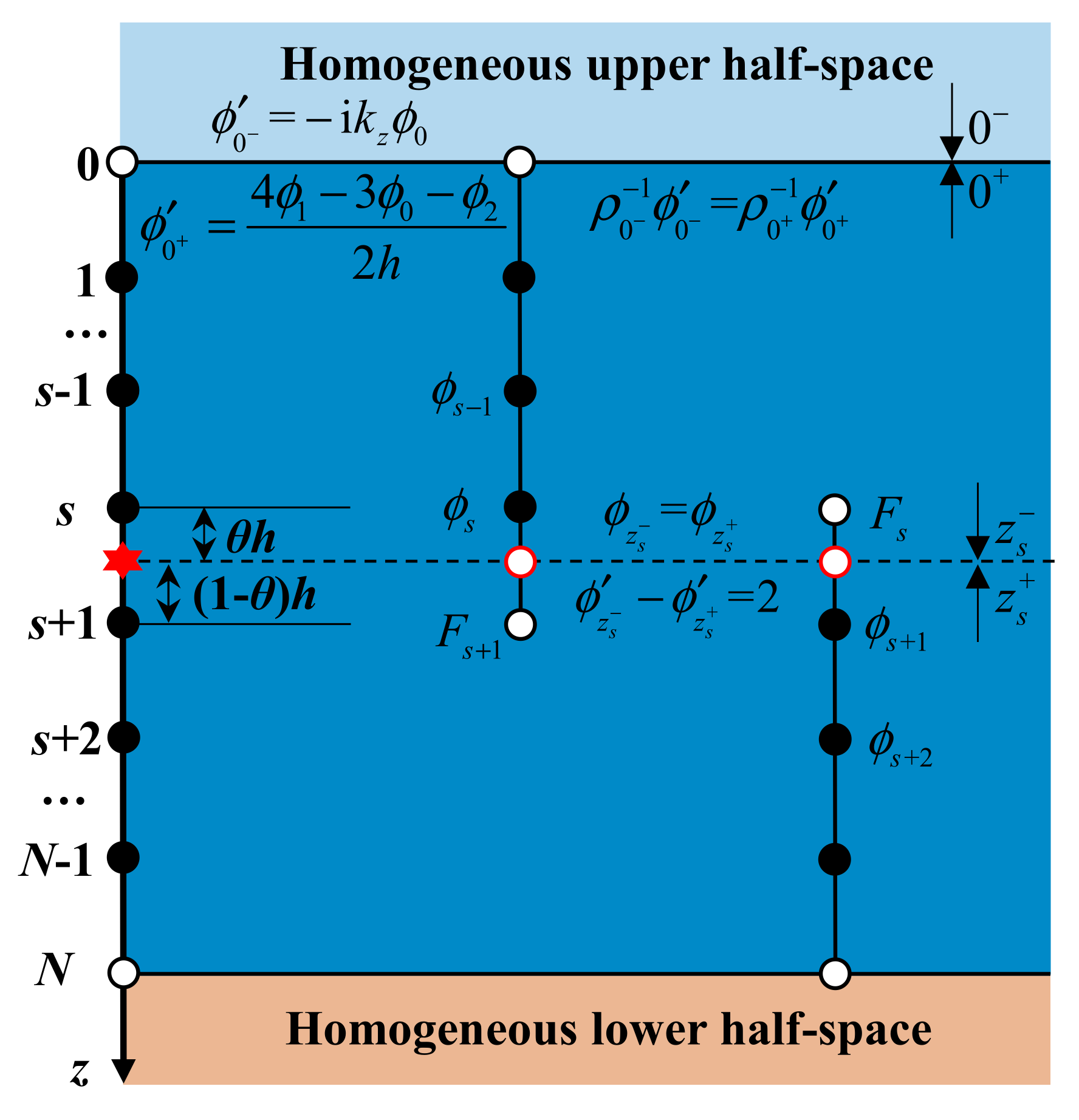
As shown in Figure 1, the kernel ($\varphi$) is continuous at the upper boundary, and its derivative with respect to the depth (${\varphi }^{\prime }$) satisfies

$${\rho }_{0^{+}}^{-1}{{\varphi }^{\prime }}_{0^{+}}={\rho }_{0^{-}}^{-1}{{\varphi }^{\prime }}_{0^{-}}$$

(5)

where the subscripts “$0^{-}$” and “$0^{+}$” represent the upper and lower surfaces, respectively, of the upper boundary (grid point 0). The derivative inside the water (${{\varphi }^{\prime }}_{0^{+}}$) can be calculated using kernels on the interior grid points by the FDM. To calculate the derivative outside the water (${{\varphi }^{\prime }}_{0^{-}}$), considering the homogeneous properties of the half-space above the water column, Equation (4) can be changed to the plane wave equation away from the source:

$${\partial }^2\varphi /\partial z^2+k_z^2\varphi =0$$

(6)

Because only upgoing waves are present in the upper half-space, the solution of Equation (6) is:

$$\varphi =C{e}^{-\mathrm{i}{k}_{z,0^{-}}z}$$

(7)

where C is a constant. Then, ${{\varphi }^{\prime }}_{0^{-}}$ can be expressed by the kernel on the upper boundary:

$${{\varphi }^{\prime }}_{0^{-}}=-\mathrm{i}{k}_{z,0^{-}}{\varphi }_0$$

(8)

The lower boundary conditions at grid point N can be treated as symmetric (only downgoing waves are present) to the upper boundary conditions.

The source interface conditions state that the kernel must be continuous (${\varphi }_{z_s^{-}}={\varphi }_{z_s^{+}}$), and the derivative of the kernel follows the jump condition. Let $z_s^{-}=z_s-\epsilon$ and $z_s^{+}=z_s+\epsilon$, where $\epsilon \to 0$. Then, Equation (4) is integrated over depth z from $z_s^{-}$ to $z_s^{+}$ along the z-axis through the source. We can obtain the jump condition of the derivative of the kernel:

$${{\varphi }^{\prime }}_{z_s^{-}}-{{\varphi }^{\prime }}_{z_s^{+}}=2$$

(9)

2.2. The FDM for the Depth Equaiton

As shown in Figure 1, equally-spaced grids in the depth direction are used in this paper, and h is the grid step size in meters. At the interior grid points far from the boundaries and source, the second derivatives in Equation (4) can be discretized using the standard 2nd-order accuracy FD scheme:

$${\left[\rho \frac{\partial }{\partial z}\left(\frac{1}{\rho }\frac{\partial \varphi }{\partial z}\right)\right]}_i=\frac{{\rho }_i}{h}\left[{\left(\frac{1}{\rho }\frac{\partial \varphi }{\partial z}\right)}_{i+1/2}-{\left(\frac{1}{\rho }\frac{\partial \varphi }{\partial z}\right)}_{i-1/2}\right]=\frac{{\rho }_i}{h}\left(\frac{{\varphi }_{i+1}-{\varphi }_i}{{\rho }_{i+1/2}h}-\frac{{\varphi }_i-{\varphi }_{i-1}}{{\rho }_{i-1/2}h}\right)$$

(10)

where ${\rho }_{i+1/2}=\rho \left(z_{i+1/2}\right)$ and ${\rho }_{i-1/2}=\rho \left(z_{i-1/2}\right)$. Then, the discretized depth equation at interior points can be expressed as:

$$\frac{1}{h^2}\frac{{\rho }_i}{{\rho }_{i-1/2}}{\varphi }_{i-1}+\left[\left(k^2-k_r^2\right)-\frac{1}{h^2}\left(\frac{{\rho }_i}{{\rho }_{i-1/2}}+\frac{{\rho }_i}{{\rho }_{i+1/2}}\right)\right]{\varphi }_i+\frac{1}{h^2}\frac{{\rho }_i}{{\rho }_{i+1/2}}{\varphi }_{i+1}=0$$

(11)

At the lower surface of the upper boundary, the derivative of the kernel (${\varphi }^{\prime }$) can be approximated using the 2nd-order FD scheme:

$${{\varphi }^{\prime }}_{0^{+}}=\left(-3{\varphi }_0+4{\varphi }_1-{\varphi }_2\right)/\left(2h\right)$$

(12)

After inserting Equations (5) and (8), we can establish the equation:

$${\rho }_{0^{+}}^{-1}\left(-3{\varphi }_0+4{\varphi }_1-{\varphi }_2\right)/\left(2h\right)=-\mathrm{i}{\rho }_{0^{-}}^{-1}{k}_{z,0^{-}}{\varphi }_0$$

(13)

and we can attain the following relationship between the kernel on the upper boundary ${\varphi }_0$ and the kernels at the interior points (${\varphi }_1$ and ${\varphi }_2$):

$${\varphi }_0={\rho }_{0^{-}}\left(4{\varphi }_1-{\varphi }_2\right)/\left(3{\rho }_{0^{-}}-2i{k}_{z,0^{-}}h{\rho }_{0^{+}}\right)$$

(14)

Specifically, for the pressure-release upper boundary, we can set the density in the upper half-space to zero (${\rho }_{0^{-}}=0$, and thus, ${\varphi }_0=0$). The lower boundary can be treated as symmetrical with respect to the upper boundary, and thus, we can derive the following relationship between the kernel on the lower boundary (${\varphi }_N$) and the kernels at the interior points (${\varphi }_{N-1}$ and ${\varphi }_{N-2}$):

$${\varphi }_N={\rho }_{N^{+}}\left(4{\varphi }_{N-1}-{\varphi }_{N-2}\right)/\left(3{\rho }_{N^{+}}-2i{k}_{z,N^{+}}h{\rho }_{N^{-}}\right)$$

(15)

At grid points near the source interface, the MIB method is used to form the FD schemes. The MIB is a numerical method that can treat discontinuous interfaces: the solution on each side of the source interface is smoothly extended beyond the interface by means of fictitious domains, and the fictitious values in the fictitious domains are determined simultaneously by enforcing the source interface conditions at the exact position of the interface [31,32]. Assuming that the source interface lies between the grid nodes s and s + 1, the interface splits this grid step into two pieces with sizes of θh at the upper part and (1 − θ)h at the lower part, where 0 ≤ θ < 1. Because the derivative is discontinuous at the source interface, the MIB method smoothly extends the solution on the upper side of the source interface beyond the interface by means of fictitious domains and sets the fictitious kernel F_s+1 at the location of grid point s + 1; symmetrically, the fictitious kernel F_s is supplied at the location of grid point s to smoothly extend the solution from the lower side of the source interface to the upper side. Using Lagrange interpolation polynomials, the kernel at the source interface can be interpolated from the upper and lower sides:

$${\varphi }_{z_s^{-}}=\theta \left(\theta -1\right){\varphi }_{s-1}/2+\left(1-{\theta }^2\right){\varphi }_s+\theta \left(\theta +1\right)F_{s+1}/2$$

(16)

$${\varphi }_{z_s^{+}}=\left[1+\theta \left(\theta -3\right)/2\right]F_s-\theta \left(\theta -2\right){\varphi }_{s+1}+\theta \left(\theta -1\right){\varphi }_{s+2}/2$$

(17)

Moreover, the derivatives of the kernel at the source interface can be approximated using the 2nd-order FD scheme from the upper and lower sides:

$${{\varphi }^{\prime }}_{z_s^{-}}={\left(2h\right)}^{-1}\left[\left(2\theta -1\right){\varphi }_{s-1}-4\theta {\varphi }_s+\left(1+2\theta \right)F_{s+1}\right]$$

(18)

$${\varphi }_{z_s^{+}}={\left(2h\right)}^{-1}\left[\left(2\theta -3\right)F_s+4\left(1-\theta \right){\varphi }_{s+1}+\left(2\theta -1\right){\varphi }_{s+2}\right]$$

(19)

Applying source interface conditions of ${\varphi }_{z_s^{-}}={\varphi }_{z_s^{+}}$ and Equation (9), the fictitious kernels in the fictitious domains can be determined simultaneously:

$$\left\{\begin{array}{l}{F}_s=\frac{-{\theta }^2{\varphi }_{s-1}+{\left(\theta +1\right)}^2{\varphi }_s-3{\theta }^2{\varphi }_{s+1}+{\theta }^2{\varphi }_{s+2}+2\theta \left(\theta +1\right)h}{1+2\theta -2{\theta }^2}\\ F_{s+1}=\frac{{\left(\theta -1\right)}^2{\varphi }_{s-1}-3{\left(\theta -1\right)}^2{\varphi }_s+{\left(\theta -2\right)}^2{\varphi }_{s+1}-{\left(\theta -1\right)}^2{\varphi }_{s+2}+2\left(\theta -2\right)\left(\theta -1\right)h}{1+2\theta -2{\theta }^2}\end{array}\right.$$

(20)

Thus, by using the above FDM with 2nd-order accuracy, a linear system of the discretized depth equation at all grid points (excluding the boundary points 0 and N) can be obtained and solved using direct methods for solving linear systems:

$$A\varphi =b,A\in {\mathrm{C}}^{\left(N-1\right)\times \left(N-1\right)},\varphi ,b\in {\mathrm{C}}^{N-1}$$

(21)

where

$$b_i=\left\{\begin{array}{cc}\frac{-1}{h}\frac{{\rho }_s}{{\rho }_{s+1/2}}\frac{2\left(\theta -2\right)\left(\theta -1\right)}{1+2\theta -2{\theta }^2},& i=s\\ \frac{-1}{h}\frac{{\rho }_{s+1}}{{\rho }_{s+1/2}}\frac{2\theta \left(\theta +1\right)}{1+2\theta -2{\theta }^2},& i=s+1\\ 0,& else\end{array}\right.$$

(22)

and

$$A=\left(\begin{array}{cccccccc}{a}_{1,1}& a_{1,2}& & & & & & \\ a_{2,1}& a_{2,2}& a_{2,3}& & & & 0& \\ & \ddots & \ddots & \ddots & & & & \\ & & a_{s,s-1}& a_{s,s}& a_{s,s+1}& a_{s,s+2}& & \\ & & a_{s+1,s-1}& a_{s+1,s}& a_{s+1,s+1}& a_{s+1,s+2}& & \\ & & & & \ddots & \ddots & \ddots & \\ & 0& & & & a_{N-2,N-3}& a_{N-2,N-2}& a_{N-2,N-1}\\ & & & & & & a_{N-1,N-2}& a_{N-1,N-1}\end{array}\right)$$

(23)

where

$$\left\{\begin{array}{l}{a}_{1,1}=k_z^2+\frac{1}{h^2}\left(\frac{{\rho }_1}{{\rho }_{1/2}}\frac{{\rho }_{0^{-}}+2\mathrm{i}{k}_{z,0^{-}}h{\rho }_{0^{+}}}{3{\rho }_{0^{-}}-2\mathrm{i}{k}_{z,0^{-}}h{\rho }_{0^{+}}}-\frac{{\rho }_1}{{\rho }_{3/2}}\right)\\ a_{1,2}=\frac{1}{h^2}\left(\frac{{\rho }_1}{{\rho }_{3/2}}-\frac{{\rho }_1}{{\rho }_{1/2}}\frac{{\rho }_{0^{-}}}{3{\rho }_{0^{-}}-2\mathrm{i}{k}_{z,0^{-}}h{\rho }_{0^{+}}}\right)\end{array}\right.$$

(24)

$$\left\{\begin{array}{l}{a}_{N-1,N-1}=k_z^2+\frac{1}{h^2}\left(\frac{{\rho }_{N-1}}{{\rho }_{N-1/2}}\frac{{\rho }_{N^{+}}+2\mathrm{i}{k}_{z,N^{+}}h{\rho }_{N^{-}}}{3{\rho }_{N^{+}}-2\mathrm{i}{k}_{z,N^{+}}h{\rho }_{N^{-}}}-\frac{{\rho }_{N-1}}{{\rho }_{N-3/2}}\right)\\ a_{N-1,N-2}=\frac{1}{h^2}\left(\frac{{\rho }_{N-1}}{{\rho }_{N-3/2}}-\frac{{\rho }_{N-1}}{{\rho }_{N-1/2}}\frac{{\rho }_{N^{+}}}{3{\rho }_{N^{+}}-2\mathrm{i}{k}_{z,N^{+}}h{\rho }_{N^{-}}}\right)\end{array}\right.$$

(25)

$$\left\{\begin{array}{l}{a}_{s,s-1}=\frac{1}{h^2}\left(\frac{{\rho }_s}{{\rho }_{s-1/2}}+\frac{{\rho }_s}{{\rho }_{s+1/2}}\frac{{\left(\theta -1\right)}^2}{1+2\theta -2{\theta }^2}\right)\\ a_{s,s}=k_z^2-\frac{1}{h^2}\left(\frac{{\rho }_s}{{\rho }_{s-1/2}}+\frac{{\rho }_s}{{\rho }_{s+1/2}}\frac{{\left(\theta -2\right)}^2}{1+2\theta -2{\theta }^2}\right)\\ a_{s,s+1}=\frac{1}{h^2}\frac{{\rho }_s}{{\rho }_{s+1/2}}\frac{{\left(\theta -2\right)}^2}{1+2\theta -2{\theta }^2}\\ a_{s,s+2}=-\frac{1}{h^2}\frac{{\rho }_s}{{\rho }_{s+1/2}}\frac{{\left(\theta -1\right)}^2}{1+2\theta -2{\theta }^2}\end{array}\right.$$

(26)

$$\left\{\begin{array}{l}{a}_{s+1,s-1}=\frac{-1}{h^2}\frac{{\rho }_{s+1}}{{\rho }_{s+1/2}}\frac{{\theta }^2}{1+2\theta -2{\theta }^2}\\ a_{s+1,s}=\frac{1}{h^2}\frac{{\rho }_{s+1}}{{\rho }_{s+1/2}}\frac{{\left(\theta +1\right)}^2}{1+2\theta -2{\theta }^2}\\ a_{s+1,s+1}=k_z^2-\frac{1}{h^2}\left[\frac{{\rho }_{s+1}}{{\rho }_{s+3/2}}+\frac{{\rho }_{s+1}}{{\rho }_{s+1/2}}\frac{{\left(\theta +1\right)}^2}{1+2\theta -2{\theta }^2}\right]\\ a_{s+1,s+2}=\frac{1}{h^2}\left(\frac{{\rho }_{s+1}}{{\rho }_{s+3/2}}+\frac{{\rho }_{s+1}}{{\rho }_{s+1/2}}\frac{{\theta }^2}{1+2\theta -2{\theta }^2}\right)\end{array}\right.$$

(27)

$$\left\{\begin{array}{l}{a}_{i,i-1}=\frac{1}{h^2}\frac{{\rho }_i}{{\rho }_{i-1/2}}\\ a_{i,i}=k_z^2-\frac{1}{h^2}\left(\frac{{\rho }_i}{{\rho }_{i-1/2}}+\frac{{\rho }_i}{{\rho }_{i+1/2}}\right)\\ a_{i,i+1}=\frac{1}{h^2}\frac{{\rho }_i}{{\rho }_{i+1/2}}\end{array}\right.,\mathrm{where}1<i<s\mathrm{or}s+1<i<N-1$$

(28)

To improve the numerical accuracy of the kernels, a 4th-order FD scheme is also developed, which is described in Appendix A.

3. VWI Approaches

In addition to the sound pressure P, the VWI model also needs to calculate the acoustic particle velocity. According to Euler’s equation, the acoustic particle velocity can be calculated from the spatial gradient of pressure [33]:

$$V\left(r,z\right)=\left[U\left(r,z\right),W\left(r,z\right)\right]=\frac{1}{\mathrm{i}\rho \omega }\nabla P\left(r,z\right)$$

(29)

In the present VWI model, the particle velocity at any position in the acoustic field is directly calculated using the wavenumber integration method without a two-dimensional grid. Using Equations (3) and (29), the horizontal and vertical components of the particle velocity can be expressed as follows:

$$U=\frac{1}{\mathrm{i}\rho \omega }{P}_r{}^{\prime }=\frac{-1}{\mathrm{i}\rho \omega }{\displaystyle {\int }_0^{\infty }\varphi \left(k_r,z\right)J_1\left(k_{r}r\right)}{k}_r^{2}d{k}_r$$

(30)

$$W=\frac{1}{\mathrm{i}\rho \omega }{P^{\prime }}_z={\displaystyle {\int }_0^{\infty }w\left(k_r,z\right)}{J}_0\left(k_{r}r\right)k_{r}d{k}_r$$

(31)

where $P_r{}^{\prime }=\partial P/\partial r$, $P_z{}^{\prime }=\partial P/\partial z$, J₁ is the first-order Bessel function of the first kind ($\partial J_0\left(k_{r}r\right)/\partial r=-k_r{J}_1\left(k_{r}r\right)$), and $w={\varphi }^{\prime }/\left(\mathrm{i}\rho \omega \right)$ is the kernel of the vertical component of the particle velocity and can also be calculated using the FDM. For the 2nd-order FD scheme:

$${{\varphi }^{\prime }}_i=\frac{1}{2h}\left\{\begin{array}{l}{F}_{s+1}-{\varphi }_{s-1},i=s\\ {\varphi }_{s+2}-F_s,i=s+1\\ {\varphi }_{i+1}-{\varphi }_{i-1},else\end{array}\right.$$

(32)

For the 4th-order FD scheme:

$${{\varphi }^{\prime }}_i=\frac{1}{12h}\left\{\begin{array}{l}-3{\varphi }_0-10{\varphi }_1+18{\varphi }_2-6{\varphi }_3+{\varphi }_4,i=1\\ 3F_{s+1}+10{\varphi }_s-18{\varphi }_{s-1}+6{\varphi }_{s-2}-{\varphi }_{s-3},i=s\\ -3F_s-10{\varphi }_{s+1}+18{\varphi }_{s+2}-6{\varphi }_{s+3}+{\varphi }_{s+4},i=s+1\\ 3{\varphi }_N+10{\varphi }_{N-1}-18{\varphi }_{N-2}+6{\varphi }_{N-3}-{\varphi }_{N-4},i=N-1\\ 8\left({\varphi }_{i+1}-{\varphi }_{i-1}\right)-\left({\varphi }_{i+2}-{\varphi }_{i-2}\right),else\end{array}\right.$$

(33)

In the cycles of wavenumber integration, the zero-order Bessel function of the first kind J₀(k_rr) can be shared by the integrals of the pressure P in Equation (3) and the vertical component of the particle velocity W in Equation (31).

3.1. Algorithm Parameters

To numerically evaluate the wavenumber integrals in Equations (3), (30) and (31), the kernel needs to be evaluated at discrete horizontal wavenumbers. In this paper, k_r ∈ [0, k_max] is discretized equidistantly to N_k cells, and the kernel at the midpoint of each cell is used as the average value of that cell for wavenumber integration. Thus, discretized horizontal wavenumbers used to solve the depth equation can be expressed as:

$$k_{r,n}=\left(n-1/2\right)\Delta k_r,n=1,2,\dots ,N_k$$

(34)

where $\Delta k_r$ is the horizontal wavenumber step size. To achieve more accurate integrals, $\Delta k_r$ should be small enough to avoid aliasing and wrap-around effects [2], which means that a sufficient number of sampling points is needed at the maximum range R_max. In this paper, the horizontal wavenumber step size is estimated using:

$$\Delta k_r=2\pi /\left(n_R{R}_{\max }\right)$$

(35)

where n_R is the number of samples of the horizontal wavenumber in each 2π period (the Bessel functions exhibit periodic oscillations similar to the cosine function) at r = R_max. Then, the total number of samples of the horizontal wavenumber can be calculated by $N_k=k_{\max }/\Delta k_r$, where $k_{\max }$ is the finite maximum value of the horizontal wavenumber used to truncate the range of the infinite Sommerfeld integrals.

In addition, to avoid the vertical wavenumber k_z = 0, the integration path is commonly moved into the complex plane [34], which means that:

$$k_n=k_{r,n}-i{\epsilon }_k$$

(36)

where ${\epsilon }_k=3\Delta k_r/\left(2\mathsf{\pi }{\log }_{10}\mathrm{e}\right)$ and e is the natural constant. Then, the discrete wavenumber integrals of Equations (3) and (29) can be expressed as:

$$P\left(r,z\right)=\Delta k_r{\displaystyle \sum _{n=1}^{N_k}\varphi \left(k_n,z\right)J_0\left(k_{n}r\right)k_n}$$

(37)

$$V\left(r,z\right)=\Delta k_r\left(\frac{\mathrm{i}}{\rho \omega }{\displaystyle \sum _{n=1}^{N_k}\varphi \left(k_n,z\right)J_1\left(k_{n}r\right)k_n^2},{\displaystyle \sum _{n=1}^{N_k}w\left(k_n,z\right)J_0\left(k_{n}r\right)k_n}\right)$$

(38)

3.2. Vector Sound Intensity

After the particle velocity field is calculated using the VWI method, the TASI streamlines can be traced to visualize the time-independent energy flow in the acoustic field. Although sound intensity streamlines have been applied in several studies [35,36,37], these streamlines are rarely shown together with the TL contours to better understand the TL distribution.

For a steady-state (time-harmonic) sound field, the TASI I can be obtained by temporally averaging the instantaneous intensity over one time period (T = 2π/ω), which can be expressed as [35]:

$$I=\frac{1}{2}\mathrm{Re}\left\{P{V}^{*}\right\}=\frac{1}{2}\mathrm{Re}\left\{P^{*}V\right\}$$

(39)

Additionally, the two components of I can be expressed as:

$$I_r=\frac{1}{2}\mathrm{Re}\left\{P{V}_r^{*}\right\}\mathrm{and}{I}_z=\frac{1}{2}\mathrm{Re}\left\{P{V}_z^{*}\right\}$$

(40)

The TASI governs the net transport of energy, whose direction is proportional to the spatial gradient of the pressure phase and perpendicular to the resultant wave fronts (surfaces of the constant-pressure phase). The TASI streamline curves are tangent to the direction of the local TASI vector at every point [35,38], and these streamlines can describe the way in which sound energy is transferred, physically coming only from the sound source and propagating along the streamlines to infinity [39].

4. Benchmarking for Vector Acoustic Fields

Four benchmark cases were used to test the present VWI model: the free acoustic field, the ideal fluid waveguide, the Bucker waveguide, and the Munk waveguide. Moreover, the TASI vectors and streamlines are calculated and traced to visualize the time-averaged energy flow path, and the TL distribution is interpreted from the perspective of streamlines.

4.1. The Free Acoustic Field

If the acoustic environment is a homogeneous and unbounded medium (free space), the solution of the acoustic Helmholtz equation is analytical and can be expressed using the Sommerfeld–Weyl integral [2] (page 88):

$$P\left(r,z\right)=\frac{e^{\mathrm{i}kR}}{R}={\displaystyle {\int }_0^{\infty }\frac{\mathrm{i}}{k_z}{\mathrm{e}}^{\mathrm{i}{k}_z\left|z-z_s\right|}{J}_0\left(k_{r}r\right)k_{r}d{k}_r}$$

(41)

where $R=\sqrt{r^2+{\left(z-z_s\right)}^2}$ is the distance from the source point (0, z_s) to the position (r, z). Moreover, the exact kernel is:

$${\varphi }^{\mathrm{Exact}}=\mathrm{i}{\mathrm{e}}^{\mathrm{i}{k}_z\left|z-z_s\right|}/k_z$$

(42)

which can be used to verify the numerical solution of the kernel solved by using the FDM.

Herein, the thickness of the uniform medium (water) is 5000 m, the sound speed and density of the medium are 1500 m/s and 1 g/cm³, respectively, no attenuation occurs within the medium, and the properties of the medium in the upper and lower half-space are the same as those of the water. The depths of the sound source and the receiver are 2500 m and 20 m, respectively, the largest receiver range is 24 km, and the source frequency is 5 Hz. The interval step size in the range direction is 25 m, and n_R = 10 and k_max = 10 k_ref, where k_ref = 2πf/c_ref is the reference wavenumber and c_ref = 1500 m/s is the reference sound speed.

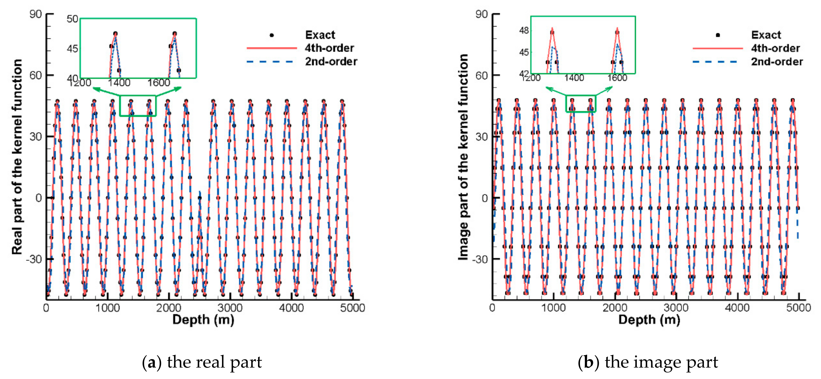
First, the FDM is verified using Equation (42). Setting the grid step size in the depth direction to h = 20 m, comparisons of the kernel (k_r = k_r,1) obtained using the exact formula and the 2nd- and 4th-order FD schemes are shown in Figure 2a,b, demonstrating that the three results agree well and that the solutions of the 4th-order FD scheme are more accurate than those of the 2nd-order FD scheme.

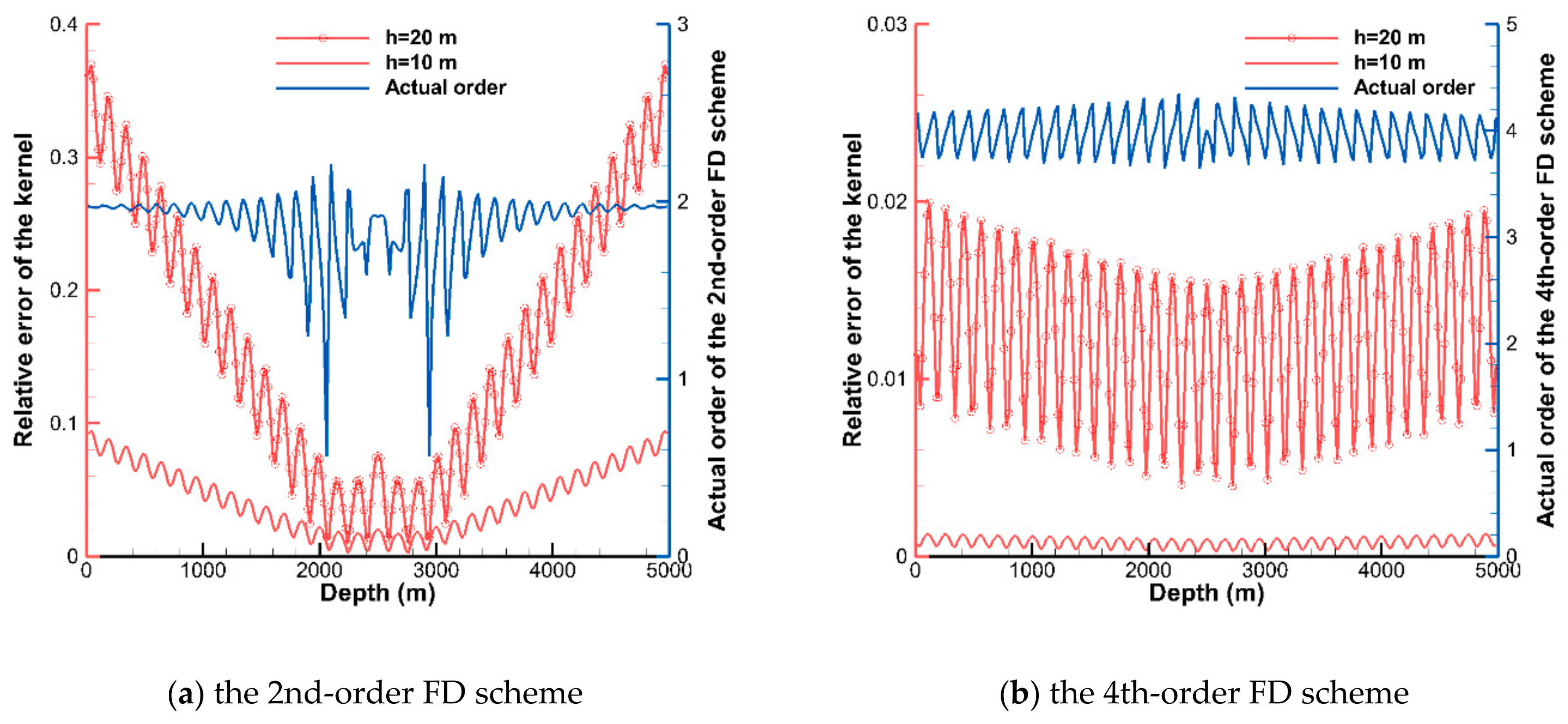
Furthermore, the actual orders of the formal 2nd- and 4th-order FD schemes were tested. The relative error of the kernel at the ith grid point can be expressed as:

$$E_i\left(h\right)=\left|{\varphi }_i^{\mathrm{FDM}}-{\varphi }_i^{\mathrm{Exact}}\right|/\left|{\varphi }_i^{\mathrm{Exact}}\right|$$

(43)

where ${\varphi }_i^{\mathrm{FDM}}$ is the numerical solution of the kernel on grid point i and ${\varphi }_i^{\mathrm{Exact}}$ is the exact solution. In this paper, two grid size steps (in the depth direction) of h₁ = 20 m and h₂ = 10 m are used to solve the depth equation. Then, at the depth of z = ih₁ = 2ih₂, the actual orders of the FD schemes can be calculated using:

$$n\left(z\right)=\frac{{\log }_e\left[E_i\left(h_1\right)/E_{2i}\left(h_2\right)\right]}{{\log }_e\left(h_1/h_2\right)}$$

(44)

Figure 3a,b show the relative errors of the kernel and actual orders with respect to the formal 2nd- and 4th-order FD schemes (k_r = k_r,1), respectively, demonstrating that the relative errors can be decreased by reducing the grid step size; the relative errors near the source depth (2500 m) are smaller than those near the boundaries; the 4th-order FD scheme has smaller relative errors than the 2nd-order FD scheme; and the actual orders of the 2nd- and 4th-order FD schemes are close to their formal orders. It is worth pointing out that the MIB method exhibits good performance at the discontinuous source interface, meaning that the actual orders of the FD schemes do not decrease near the source interface.

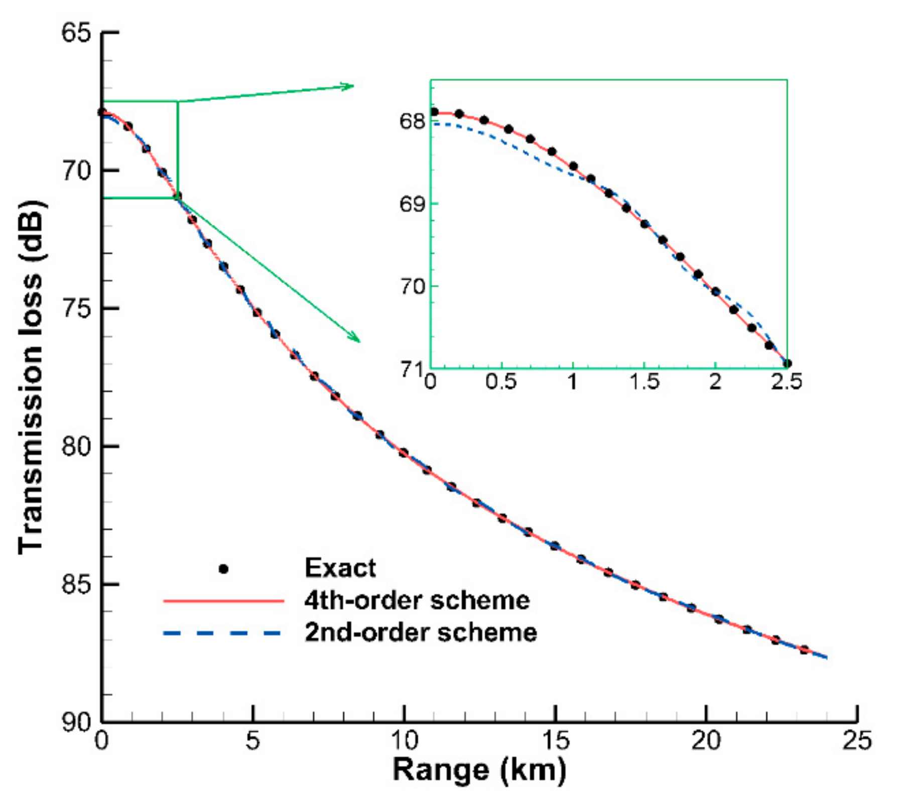
Figure 4 shows the TL curves along the receiver line z = 20 m, where TL = −20 log₁₀|P| (in dB) and |P| denotes the magnitude of the complex pressure P. The solutions of the 2nd- and 4th-order FD schemes (h = 20 m) match the exact analytical formula well in general, and the curve of the 4th-order FD scheme is closer to that of the exact formula than that of the 2nd-order FD scheme.

Figure 5 plots the TL contours and TASI streamlines obtained from the VWI model using the 2nd-order FD scheme (a) and the 4th-order FD scheme (b). In both figures, the TL contour lines are approximately concentric circles (the 4th-order scheme is more accurate than the 2nd-order scheme), whereas the TASI streamlines are straight lines from the source point to infinity, which is consistent with the characteristics of spherical waves in free space.

4.2. The Ideal Fluid Waveguide

The ideal fluid waveguide is represented by a range-independent homogeneous water column with pressure-release upper and lower boundaries [2] (page 102). The density and sound speed of the water are ρ_w = 1 g/cm³ and c_w = 1500 m/s, respectively, and the densities of the medium in the upper and lower half-spaces are both 0 g/cm³. The parameters of the sound field are as follows: the depth of the seabed is 100 m, the depths of the sound source and receiver line are 35 m and 25 m, respectively, the largest receiver range is 3 km, and the source frequency is 20 Hz. In the VWI model, n_R = 10 and k_max = 10 k_ref. The interval step sizes in the range and depth directions are both 5 m.

The image method can be used to calculate the theoretical solutions of the ideal fluid waveguide, and the acoustic pressure can be expressed using the summation of the physical source and an infinite number of image sources as follows (in this paper, the summations of the image method are truncated at m = 500):

$$P\left(r,z\right)={\displaystyle \sum _{m=1}^{\infty }\left(\frac{e^{ik{R}_{m1}}}{R_{m1}}-\frac{e^{ik{R}_{m2}}}{R_{m2}}-\frac{e^{ik{R}_{m3}}}{R_{m3}}+\frac{e^{ik{R}_{m4}}}{R_{m4}}\right)}$$

(45)

with

$$R_{mn}=\sqrt{r^2+{\left(z-z_{mn}\right)}^2},n=1,2,3,4$$

where

$$z_{m1}=2\left(m-1\right)H+z_s,z_{m2}=2mH-z_s,z_{m3}=-z_{m1},\mathrm{and}{z}_{m4}=-z_{m2}$$

and H is the depth of the seabed in meters.

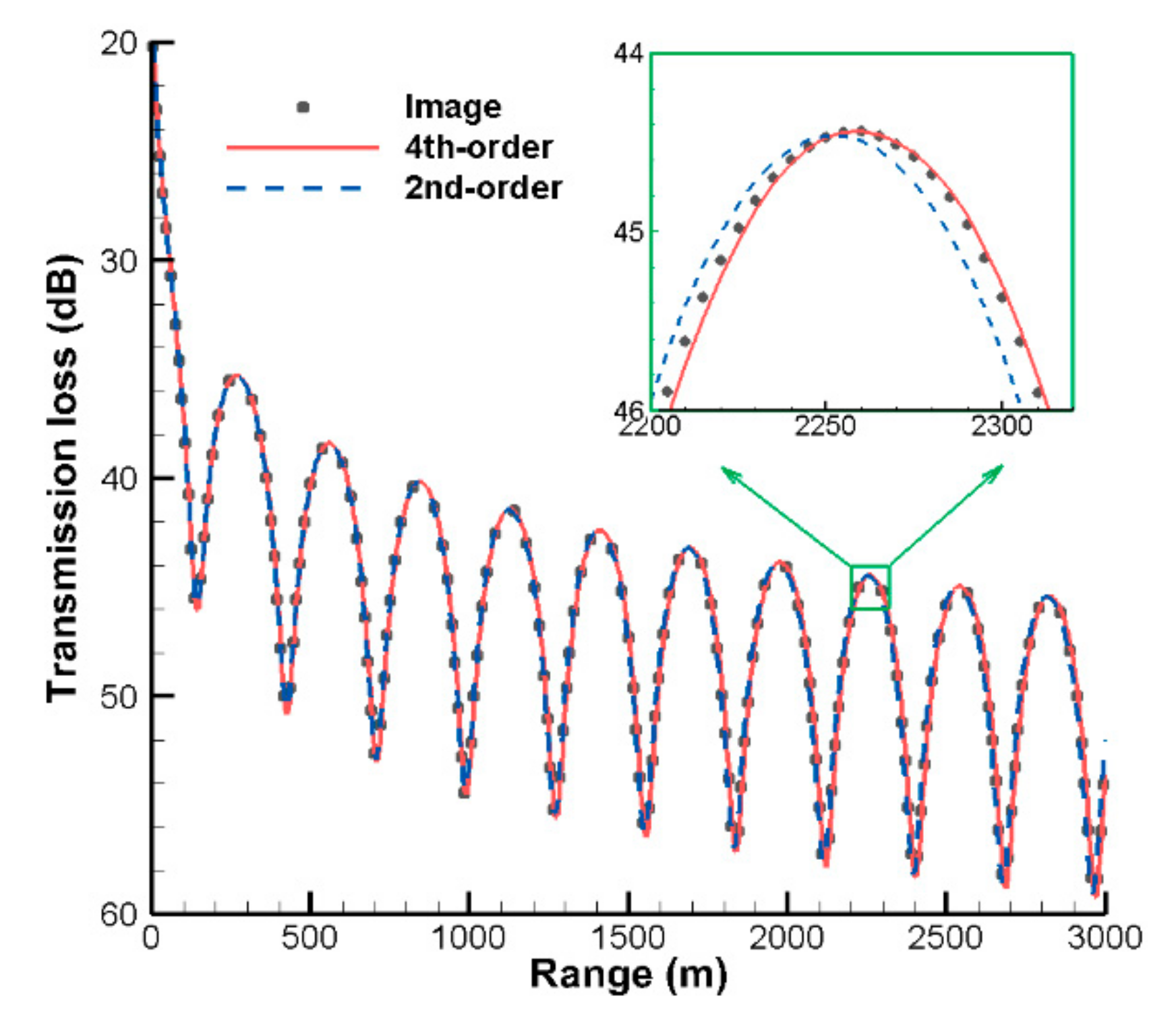
Figure 6 shows the TL curves along the receiver line calculated by the image method and the present VWI model using the 2nd- and 4th-order FD schemes. The three curves generally match well. Moreover, at the peaks and troughs of the curves, the solutions of the 4th-order FDM are closer to those of the image method than those of the 2nd-order FDM.

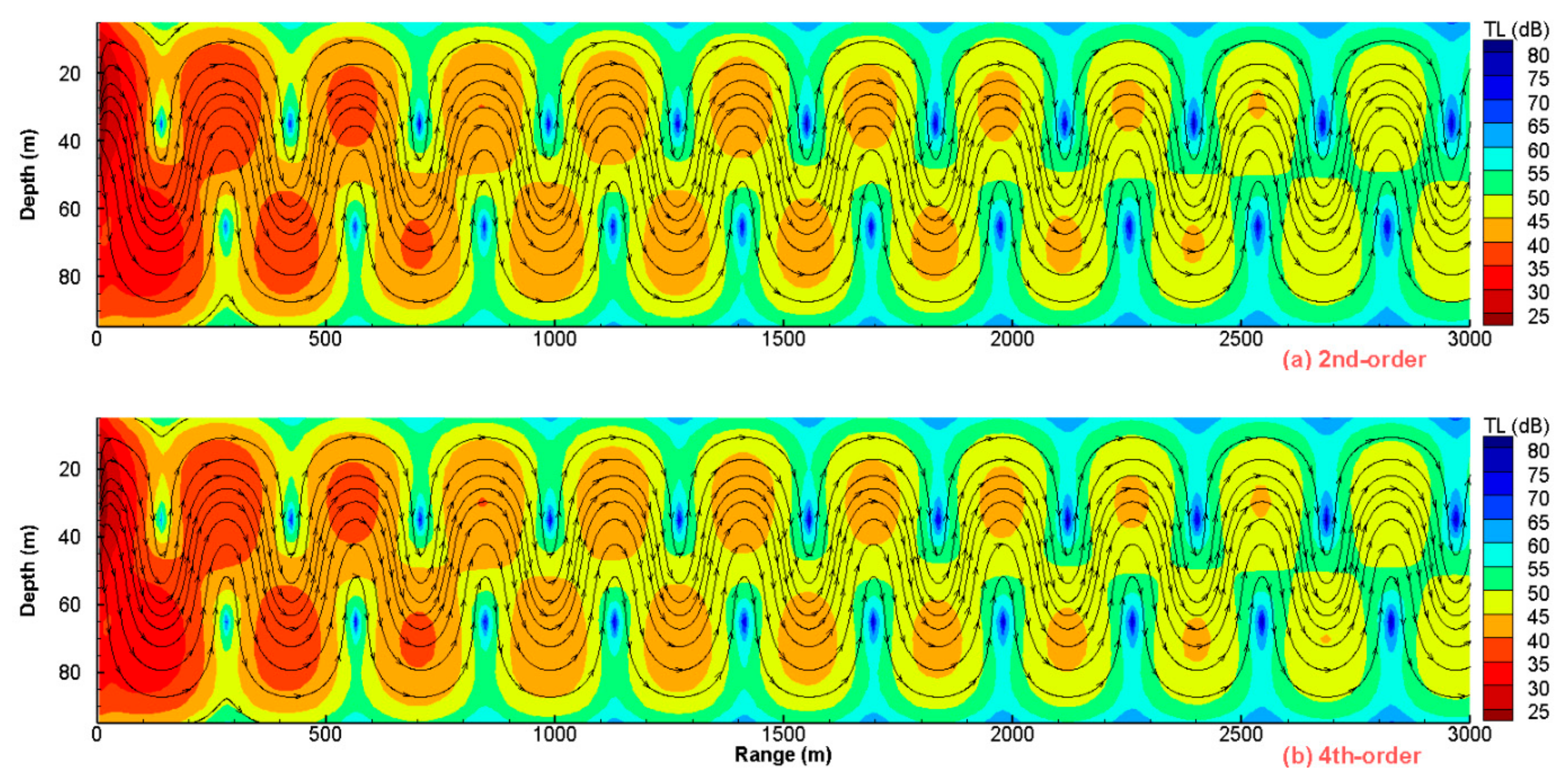
The TL contours and TASI streamlines obtained from the present VWI model using the 2nd- and 4th-order FD schemes are shown in Figure 7a,b, respectively, and they match well throughout the whole field. The main characteristic of the sound field is that the TASI streamlines are periodic in the range direction.

4.3. The Bucker Waveguide

The Bucker waveguide consists of a shallow water waveguide containing a bilinear sound speed (in m/s) profile in the water column [40]:

$$c\left(z\right)=1498+\left|120-z\right|/60$$

(46)

The depth of the water is 240 m, and the density of the water is ρ_w = 1.0 g/cm³. The density of the medium in the upper half-space is 0 g/cm³, whereas the homogeneous lower half-space of the penetrable sediment layer has a sound speed of 1505 m/s and a density of 2.1 g/cm³, and no attenuation occurs in this problem. The depths of the sound source and the receiver line are 30 m and 90 m, respectively, the largest receiver range is 2 km, and the source frequency is 100 Hz. In the VWI model, n_R = 10 and k_max = 10 k_ref. The interval step sizes in the range and depth directions are both 1 m. Because the density contrast in this waveguide yields a significant number of virtual modes close to the real wavenumber axis, normal mode models ignoring the continuous spectrum cannot provide accurate solutions. Alternatively, wavenumber integration models have no restrictions on the density contrast and are therefore capable of providing exact solutions for this environment [2] (page 300).

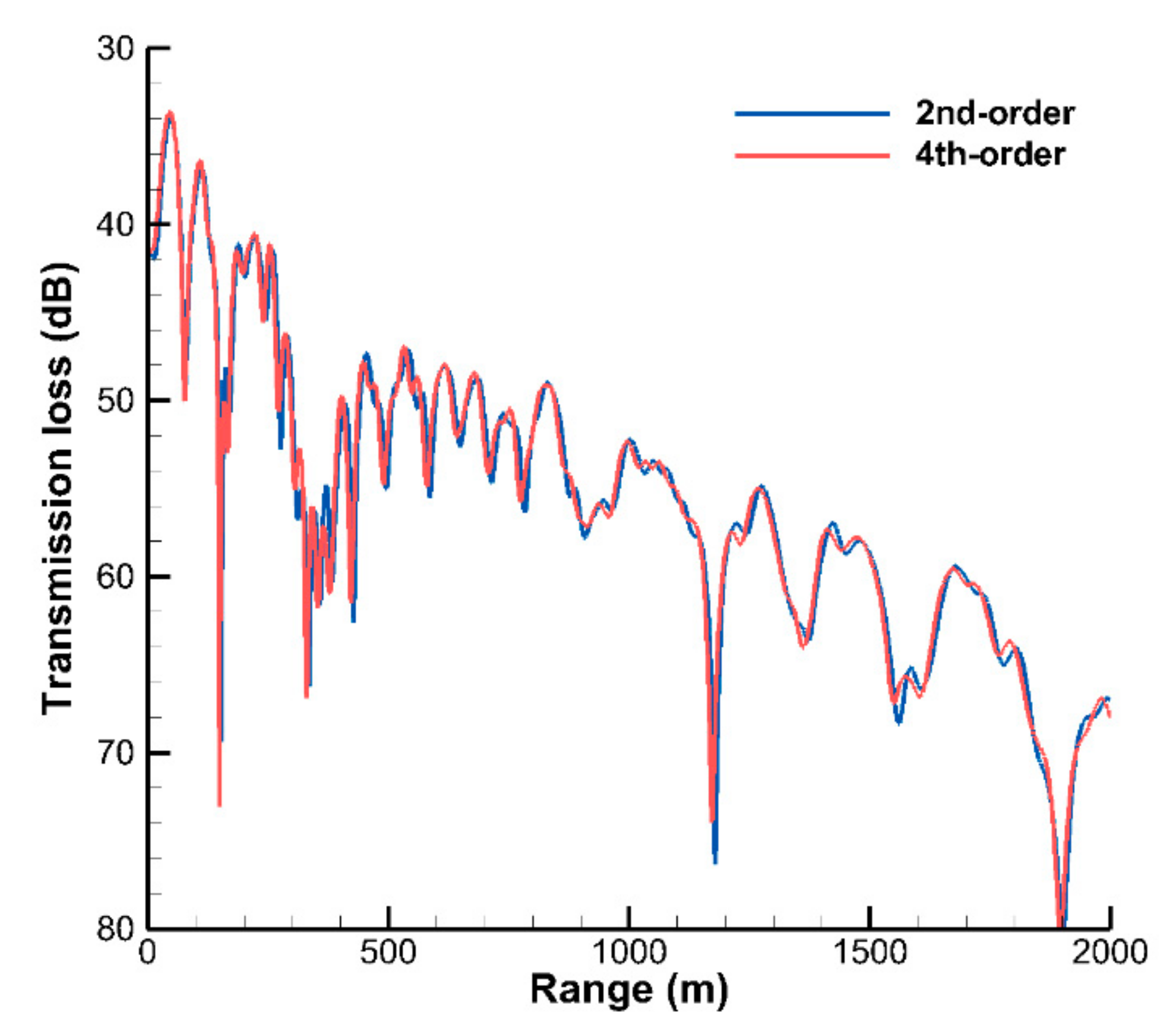
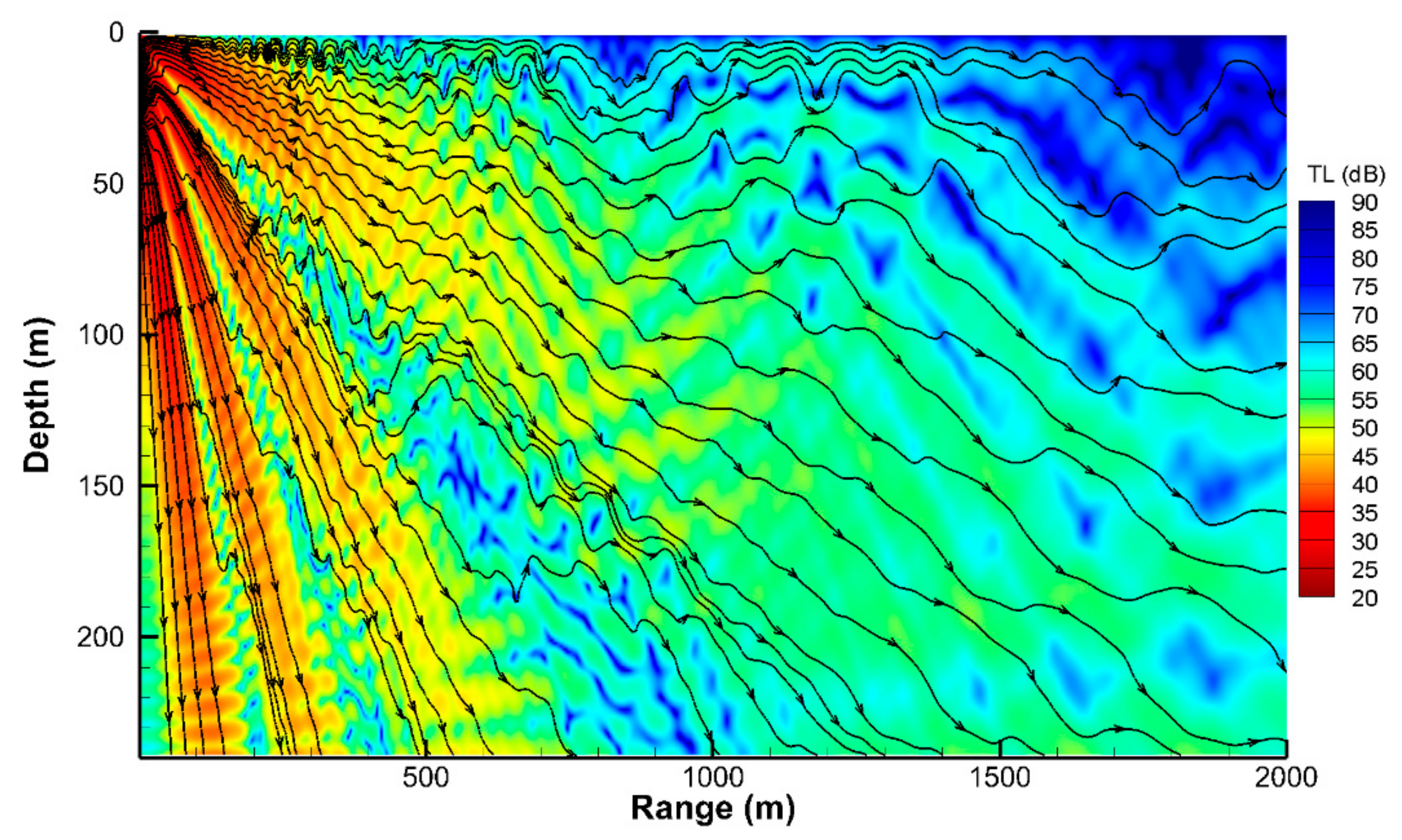
Figure 8 shows the TL curves along the receiver line calculated by the present VWI model using the 2nd- and 4th-order FD schemes, demonstrating that the two curves match well in all ranges. Figure 9 shows the TL contours obtained from the present VWI model using the 4th-order FDM, revealing that the acoustic regions with denser TASI streamlines have a smaller TL, which means that the energy distribution in the sound field is not uniform.

4.4. The Munk Waveguide

The Munk waveguide has the following analytical sound speed (in m/s) profile in water [2] (page 356):

$$c\left(z\right)=1500\left[1+0.00737\left(\tilde{z}-1+e^{-\tilde{z}}\right)\right]$$

(47)

where the scaled depth $\tilde{z}=2\left(z-1300\right)/1300$. The depth of the water is 5000 m, and the density of the water is ρ_w = 1.0 g/cm³. The density of the medium in the upper half-space is 0 g/cm³, whereas the homogeneous lower half-space of the penetrable sediment layer has a sound speed of 1600 m/s, a density of 1.8 g/cm³, and an attenuation rate of 0.8 dB/λ. The depths of the sound source and the receiver line are both 100 m, and the source frequency is 50 Hz. In the VWI model, n_R = 8 and k_max = k_ref. The interval step sizes in the range and depth directions are 300 m and 3.75 m, respectively.

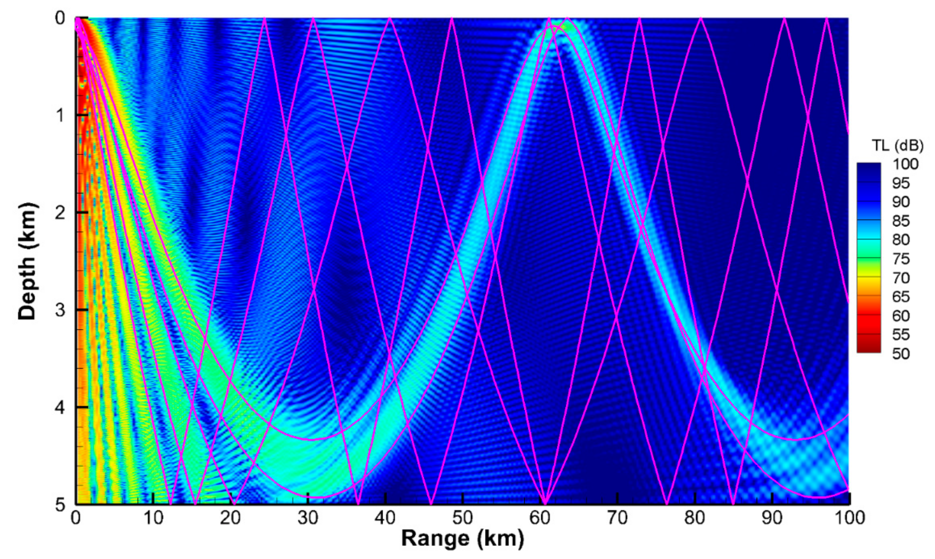
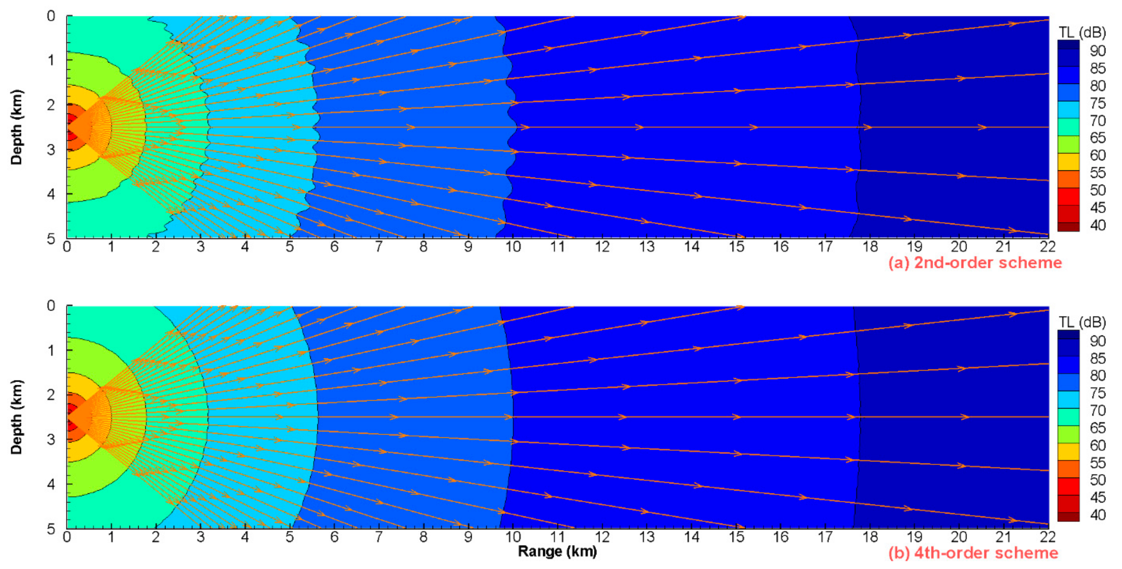
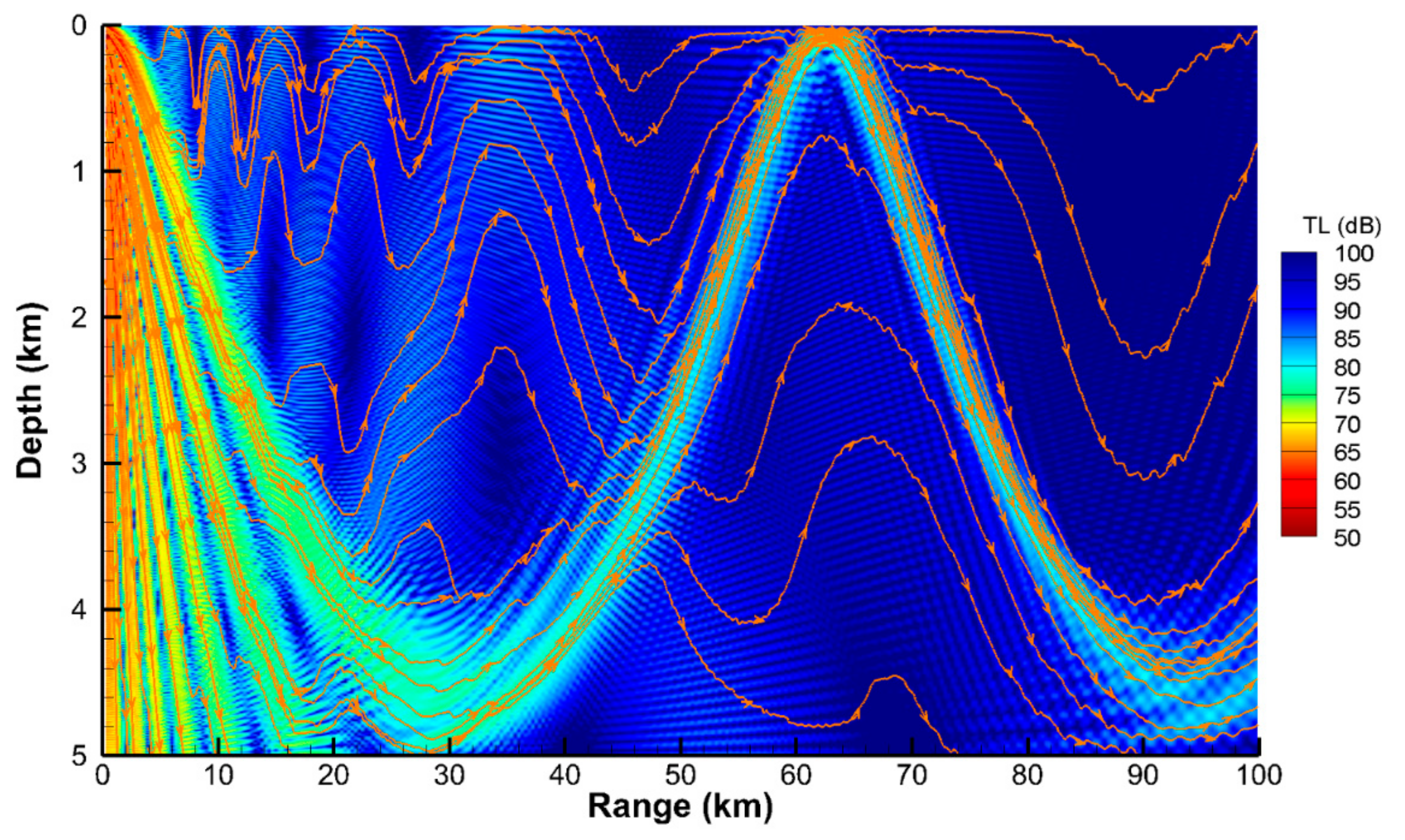
Figure 10 shows the TL contours obtained from the present VWI model using the 2nd-order FDM and the acoustic rays calculated using the BELLHOP model in the acoustic toolbox [41]. Figure 11 shows the TL contours and TASI streamlines obtained from the VWI model using the 4th-order FDM, indicating that the acoustic regions with denser TASI streamlines have a smaller TL, and the regions through which the energy flow is concentrated form zones of sound convergence.

Moreover, the TL contours in Figure 10 and Figure 11 match well, but the acoustic rays are significantly different from the TASI streamlines due to the following reasons. First, the TASI streamlines are calculated using the sound field solutions of the vector acoustic model, but the geometric rays are traced to calculate the solutions of the acoustic field. Second, because only one TASI vector direction may exist at any point in the field, the TASI streamlines cannot intersect; in contrast, the geometric rays can intersect among the multipath arrivals of propagating wavefronts in an ocean-like waveguide. Third, the TASI streamlines can accurately visualize the time-averaged energy flux, whereas the geometric rays intuitively visualize the approximate propagation of an acoustic field from the source to a receiver and do not include the diffracted components of the field.

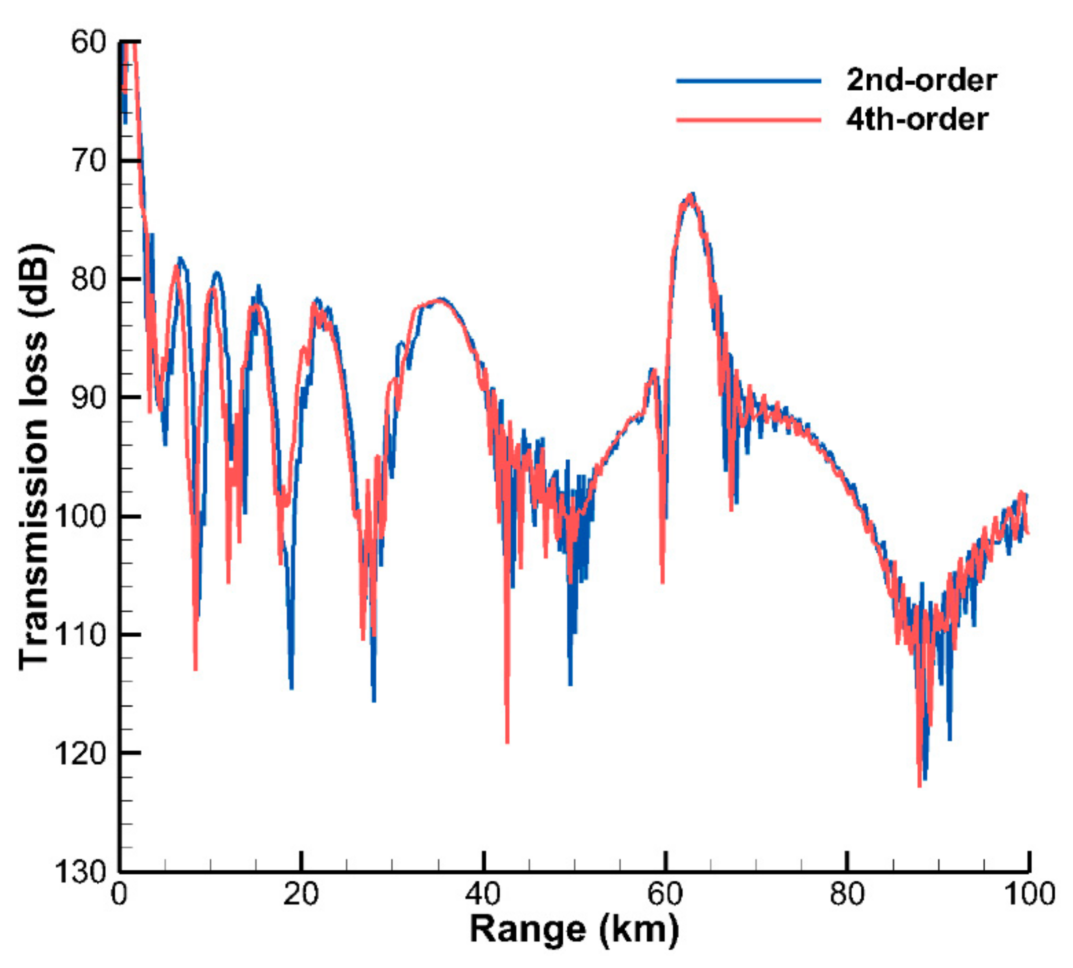
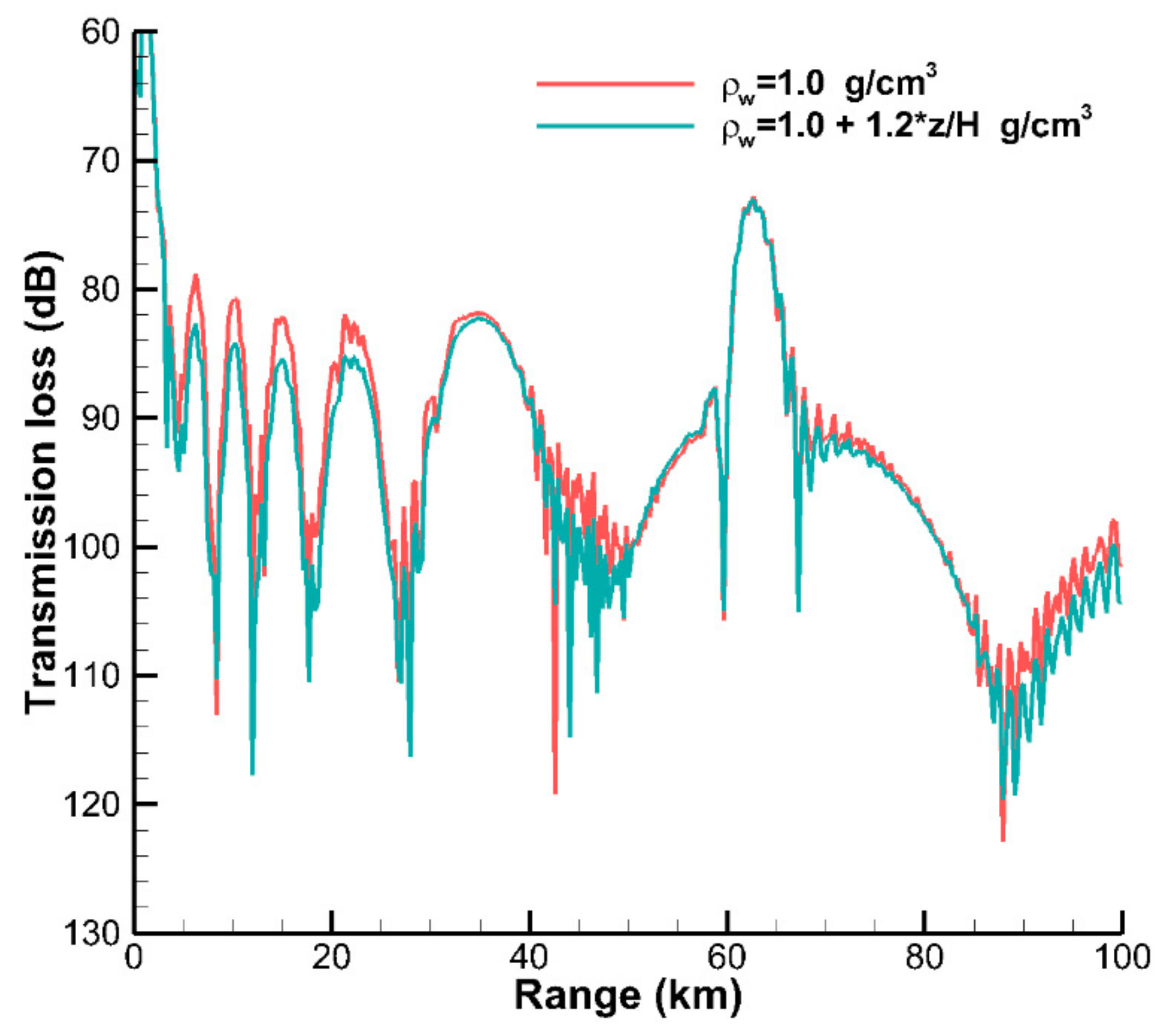
Figure 12 shows the TL curves along the receiver line calculated by the present VWI model using the 2nd- and 4th-order FD schemes, and the two curves match well in all ranges. To test the effect of the density variation with depth on the acoustic field, a density profile in water is used for the Munk waveguide (other properties remain unchanged):

$${\rho }_{\mathrm{w}}\left(z\right)=1.0+1.2z/H(\mathrm{in}\mathrm{g}/{\mathrm{cm}}^3)$$

(48)

where H = 5000 m is the seabed depth. Figure 13 shows the TL curves along the receiver line for the Munk waveguide with different density profiles in water calculated by the present VWI model using the 4th-order FDM, demonstrating that the density variation of water has an important influence on the peaks and troughs of the TL curves.

5. Conclusions and Discussion

The present range-independent VWI model can serve as a benchmark vector model for other acoustic models, such as FDM models and spectral method models. Moreover, by applying the particle velocity, the TASI streamlines can be computed and displayed, thereby bettering our understanding of the TL distribution, and these TASI streamlines can also be applied to other vector acoustic models. Furthermore, the particle velocity can be used to investigate the vortex-like structure and Stokes parameters [42] of the vector acoustic field.

It should be mentioned that the present VWI model is computationally intensive because it includes three Sommerfeld integrals (the pressure and two velocity components), and the linear system of the discretized depth equation using the FDM is solved directly because it is difficult to use the efficient forward elimination and backward substitution algorithm since matrix A is not a diagonal banded form as a result of the MIB method. Thus, parallel computing techniques [43] should be applied to the VWI model in future research to accelerate the computation.

In addition to the FDM combined with the MIB method in this paper, finite element methods and spectral methods [7] with high orders of accuracy can also be used to solve the depth equation, and a performance comparison among these methods may be studied in the future. Furthermore, the MIB method shows good performance in addressing the discontinuous source interface of the one-dimensional depth equation, and thus, it is very attractive to apply the MIB method to treat seabed discontinuities in FDM models [44].

References

1. Etter, P.C. Underwater Acoustic Modeling and Simulation, 5th ed.; CRC Press: Boca Raton, FL, USA, 2018. [Google Scholar]
2. Jensen, F.B.; Kuperman, W.A.; Porter, M.B.; Schmidt, H. Computational Ocean Acoustics, 2nd ed.; Springer: New York, NY, USA, 2011. [Google Scholar]
3. Lippert, T.; Lippert, S. Modelling of pile driving noise by means of wavenumber integration. Acoust. Aust. 2012, 40, 178–182. [Google Scholar]
4. West, M.; Sack, R.A.; Walkden, F. The fast field program (FFP). A second tutorial: Application to long range sound propagation in the atmosphere. Appl. Acoust. 1991, 33, 199–228. [Google Scholar]
5. Li, Y.L.; White, M.J. New fast field programs for a multiple—Source system. J. Acoust. Soc. Am. 1994, 96, 3277. [Google Scholar] [CrossRef] [Green Version]
6. Franke, S.J.; Swenson, G.W. A brief tutorial on the fast field program (FFP) as applied to sound propagation in the air. Appl. Acoust. 1989, 27, 203–215. [Google Scholar] [CrossRef]
7. Tu, H.; Wang, Y.; Lan, Q.; Liu, W.; Xiao, W.; Ma, S. A Chebyshev-Tau spectral method for normal modes of underwater sound propagation with a layered marine environment. J. Sound Vib. 2021, 492, 115784. [Google Scholar] [CrossRef]
8. Porter, M.B. Beam tracing for two- and three-dimensional problems in ocean acoustics. J. Acoust. Soc. Am. 2019, 146, 2016–2029. [Google Scholar] [CrossRef]
9. Wang, Y.; Tu, H.; Liu, W.; Xiao, W.; Lan, Q. Application of a Chebyshev collocation method to solve a parabolic equation model of underwater acoustic propagation. Acoust. Aust. 2021, 49, 281–291. [Google Scholar] [CrossRef]
10. Liu, W.; Cheng, X.; Xiao, W.; Wang, Y.; Zhang, L. A direct high-order finite difference solution to the Helmholtz equation in ocean acoustics. In Proceedings of the OCEANS 2018, Charleston, SC, USA, 22–25 October 2018. [Google Scholar]
11. Ma, X.; Wang, Y.; Zhu, X.; Liu, W.; Lan, Q.; Xiao, W. A spectral method for two-dimensional ocean acoustic propagation. J. Mar. Sci. Eng. 2021, 9, 892. [Google Scholar] [CrossRef]
12. Eliseevnin, V.A.; Tuzhilkin, Y.I. Acoustic power flux in a waveguide. Acoust. Phys. 2001, 47, 688–694. [Google Scholar] [CrossRef]
13. Shchurov, V.A. Peculiarities of real shallow sea wave-guide vortex structure. J. Acoust. Soc. Am. 2019, 145, 525–530. [Google Scholar] [CrossRef]
14. Deal, T.J.; Smith, K.B. Reciprocity relationships in vector acoustics and their application to vector field calculations. J. Acoust. Soc. Am. 2017, 142, 523–529. [Google Scholar] [CrossRef]
15. Yu, Y.; Ling, Q.; Xu, J. Pressure and velocity cross-spectrum of normal modes in low-frequency acoustic vector field of shallow water and its application. J. Syst. Eng. Electron. 2015, 26, 241–249. [Google Scholar] [CrossRef]
16. Dall’Osto, D.R.; Dahl, P.H.; Woong Choi, J. Properties of the acoustic intensity vector field in a shallow water waveguide. J. Acoust. Soc. Am. 2012, 131, 2023–2035. [Google Scholar] [CrossRef]
17. Wang, W.; Yang, D.; Shi, J. A prediction method for acoustic intensity vector field of elastic structure in shallow water waveguide. Shock. Vib. 2020, 2020, 5389719. [Google Scholar] [CrossRef]
18. Sheng, X.L.; Mei, J.D.; Guo, Y.; Yin, J.W.; Guo, L.X. The application of vertical sound intensity in shallow and low frequency sound field. In Proceedings of the OCEANS 2011, Waikoloa, HI, USA, 19–22 September 2011. [Google Scholar]
19. Petrov, P.S.; Prants, S.V.; Petrova, T.N. Analytical Lie-algebraic solution of a 3D sound propagation problem in the ocean. Phys. Lett. A 2017, 381, 1921–1925. [Google Scholar] [CrossRef]
20. Petrov, P.N.; Petrov, P.S. Asymptotic solution for the problem of sound propagation in a shallow sea with the bathymetry described by a parametric quadratic function. J. Acoust. Soc. Am. 2019, 146, 1946–1955. [Google Scholar] [CrossRef]
21. Smith, K.B. Validating range-dependent, full-field models of the acoustic vector field in shallow water environments. J. Comput. Acoust. 2008, 16, 471–486. [Google Scholar]
22. Gulin, O.E.; Yang, D. On the certain semi-analytical models of low-frequency acoustic fields in terms of scalar-vector description. Chin. J. Acoust. 2004, 23, 58–70. [Google Scholar]
23. Han-hao, Z.; Sheng-chun, P.; Wei, L.; Hai-gang, Z. Research on acoustic vector properties in shallow water for geoacoustic parameters inversion. In Proceedings of the IEEE/OES Acoustics in Underwater Geosciences Symposium, Rio de Janeiro, Brazil, 24–26 July 2013; pp. 1–6. [Google Scholar]
24. Tu, H.; Wang, Y.; Liu, W.; Ma, X.; Xiao, W.; Lan, Q. A Chebyshev spectral method for normal mode and parabolic equation models in underwater acoustics. Math. Probl. Eng. 2020, 2020, 7461314. [Google Scholar] [CrossRef]
25. Westwood, E.K.; Koch, R.A. Elimination of branch cuts from the normal-mode solution using gradient half spaces. J. Acoust. Soc. Am. 1999, 106, 2513–2523. [Google Scholar] [CrossRef]
26. Li, Y.L.; White, M.J. A note on using the fast field program. J. Acoust. Soc. Am. 1994, 95, 3100–3102. [Google Scholar] [CrossRef]
27. Raspet, R.; Lee, S.W.; Gilbert, R.; Bong, N.; Kuester, E.; Chang, D.C.; Richards, W.F. A fast-field program for sound propagation in a layered atmosphere above an impedance ground. Acoust. Soc. Am. J. 1985, 77, 345–352. [Google Scholar] [CrossRef]
28. Robertson, J.S. A classification scheme for computational ocean acoustic benchmark problems. Appl. Acoust. 1989, 27, 65–68. [Google Scholar] [CrossRef]
29. Schmidt, H.; Tango, G. Efficient global matrix approach to the computation of synthetic seismograms. Geophys. J. R. Astron. Soc. 1986, 84, 331–359. [Google Scholar] [CrossRef]
30. Zhou, Y.C.; Wei, G.W. On the fictitious-domain and interpolation formulations of the matched interface and boundary (MIB) method. J. Comput. Phys. 2006, 219, 228–246. [Google Scholar] [CrossRef]
31. Pan, K.; Tan, Y.; Hu, H. An interpolation matched interface and boundary method for elliptic interface problems. J. Comput. Appl. Math. 2010, 234, 73–94. [Google Scholar] [CrossRef] [Green Version]
32. Kreiss, H.O.; Petersson, N.A. An embedded boundary method for the wave equation with discontinuous coefficients. SIAM J. Sci. Comput. 2006, 28, 2054–2074. [Google Scholar] [CrossRef] [Green Version]
33. Deal, T.; Smith, K. Modeling Acoustic Vector Fields for Inverse Problems. In Proceedings of the 2016 IEEE/OES China Ocean Acoustics (COA), Harbin, China, 9–11 January 2016; pp. 1–5. [Google Scholar]
34. Luo, W.; Yu, X.; Yang, X.; Zhang, R. Analytical solution based on the wavenumber integration method for the acoustic field in a Pekeris waveguide. Chin. Phys. B 2016, 25, 044302. [Google Scholar]
35. Chapman, D.M.F. Using streamlines to visualize acoustic energy flow across boundaries. J. Acoust. Soc. Am. 2008, 124, 48–56. [Google Scholar] [CrossRef] [Green Version]
36. Mann, J.A.; Tichy, J.; Romano, A.J. Instantaneous and time-averaged energy transfer in acoustic fields. J. Acoust. Soc. Am. 1987, 82, 17–30. [Google Scholar] [CrossRef]
37. Chien, C.F.; Waterhouse, R.V. Singular points of intensity streamlines in two-dimensional sound fields. J. Acoust. Soc. Am. 1997, 101, 705–712. [Google Scholar] [CrossRef]
38. Waterhouse, R.V.; Yates, T.W.; Feit, D.; Liu, Y.N. Energy streamlines of a sound source. J. Acoust. Soc. Am. 1985, 78, 758–762. [Google Scholar] [CrossRef]
39. Zhe, J. Intensity streamlines and vorticity streamlines in three-dimensional sound fields. J. Acoust. Soc. Am. 2000, 107, 725–730. [Google Scholar] [CrossRef]
40. Brooke, G.H.; Thomson, D.J. Non-local boundary conditions for high-order parabolic equation algorithms. Wave Motion 2000, 31, 117–129. [Google Scholar] [CrossRef]
41. Porter, M.B. Acoustics Toolbox. 2020. Available online: https://oalib-acoustics.org/AcousticsToolbox/index_at.html (accessed on 15 October 2021).
42. Bonnel, J.; Flamant, J.; Dall’Osto, D.R.; Le Bihan, N.; Dahl, P.H. Polarization of ocean acoustic normal modes. J. Acoust. Soc. Am. 2021, 150, 1897–1911. [Google Scholar] [CrossRef]
43. Hope, G.; Schmidt, H. A parallelization of the wavenumber integration acoustic modelling package OASES. Comput. Geosci. 2019, 23, 777–792. [Google Scholar] [CrossRef]
44. Liu, W.; Zhang, L.; Wang, W.; Wang, Y.; Ma, S.; Cheng, X.; Xiao, W. A three-dimensional finite difference model for ocean acoustic propagation and benchmarking for topographic effects. J. Acoust. Soc. Am. 2021, 150, 1140–1156. [Google Scholar] [CrossRef]
45. LeVeque, R.J. Finite Difference Methods for Ordinary and Partial Differential Equations; Society for Industrial and Applied Mathematics (SIAM): Philadelphia, PA, USA, 2007; p. 342. [Google Scholar]
46. Lele, S.K. Compact finite difference schemes with spectral-like resolution. J. Comput. Phys. 1992, 103, 16–42. [Google Scholar] [CrossRef]
47. Pan, G.; Abubakar, A.; Habashy, T.M. An effective perfectly matched layer design for acoustic fourth-order frequency-domain finite-difference scheme. Geophys. J. Int. 2012, 188, 211–222. [Google Scholar] [CrossRef] [Green Version]
Figure 1. Schematic diagram of the boundary and source interface conditions.
Jmse 09 01134 g001
Figure 2. Comparisons of the kernel (kr = kr,1, h = 20 m) obtained using the exact formula, and the 2nd- and 4th-order FD schemes.
Jmse 09 01134 g002
Figure 3. Relative errors of the kernel and actual orders of the FD schemes (kr = kr,1).
Jmse 09 01134 g003
Figure 4. TL curves along z = 20 m for the free acoustic field (h = 20 m).
Jmse 09 01134 g004
Figure 5. TL contours and TASI streamlines obtained from the VWI model (h = 20 m) for the free acoustic field using the 2nd-order FD scheme and the 4th-order FD scheme.
Jmse 09 01134 g005
Figure 6. TL curves along the receiver line (z = 25 m) for the ideal fluid waveguide.
Jmse 09 01134 g006
Figure 7. TL contours and TASI streamlines obtained from the VWI model for the ideal fluid waveguide using the 2nd-order FDM and the 4th-order FDM.
Jmse 09 01134 g007
Figure 8. TL curves along z = 90 m for the Bucker waveguide.
Jmse 09 01134 g008
Figure 9. TL contours and TASI streamlines for the Bucker waveguide (4th-order FDM).
Jmse 09 01134 g009
Figure 10. TL contours and rays obtained from the VWI model using the 2nd-order FDM and the BELLHOP model, respectively.
Jmse 09 01134 g010
Figure 11. TL contours and TASI streamlines obtained from the VWI model using the 4th-order FDM.
Jmse 09 01134 g011
Figure 12. TL curves along z = 100 m for the Munk waveguide (ρw = 1.0 g/cm3).
Jmse 09 01134 g012
Figure 13. TL curves along z = 100 m for the Munk waveguide (4th-order FDM).
Jmse 09 01134 g013
Publisher’s Note: MDPI stays neutral with regard to jurisdictional claims in published maps and institutional affiliations.