An Effective Mesh Deformation Approach for Hull Shape Design by Optimization

Abstract

A method for the morphing of surface/volume meshes suitable to be used in hydrodynamic shape optimization is proposed. Built in the OpenFOAM environment, it relies on a Laplace equation that propagates the modifications of the surface boundaries, realized by applying a free-form deformation to a subdivision surface description of the geometry, into the computational volume mesh initially built through a combination of BlockMesh with cfMesh. The feasibility and robustness of this mesh morphing technique, used as a computationally efficient pre-processing tool, is demonstrated in the case of the resistance minimization of the DTC hull. All the hull variations generated within a relatively large design space are efficiently and successfully realized, i.e., without mesh inconsistencies and quality issues, only by deforming the initial mesh of the reference geometry. Coupled with a surrogate model approach, a significant reduction in the calm water resistance, in the extent of 10%, has been achieved in a reasonable computational time.

1. Introduction

Computational fluid dynamics (CFD) methods are nowadays widely used both to predict the ship resistance at all the design stages and to realize simulation-based design by optimization (SBDO) processes directly to design high-performance hull shapes by the systematic use of numerical calculations. Thanks to the continuous progress of numerical methods together with the increase of the available computational resources, the total resistance of a ship can be quite easily predicted by using high-fidelity viscous solvers that provide a level of accuracy of the results comparable to that of towing tank experiments (see among the other [1,2,3,4,5]). Successful examples of the application of such approaches for performance predictions of both displacing and planing hulls in calm waters and in waves can be found in [6,7,8]. These results encouraged the use of CFD analyses in the context of automatic SBDO solving single and multi-objective hydrodynamic shape optimization of conventional and unconventional vessels [9,10,11,12] similar to those applied to propellers [13], combining true CFD calculations with multi-fidelity and data-fusion optimization methods [14,15,16]. Being any design-by-optimization approach a relatively complex process based on a workflow of interconnected methods sharing I/O information, the reliability and, in particular, the robustness of each step of the process is of essential importance for a fully automated design procedure. Moreover, since design-by-optimization is a time consuming method, each step needs to be as fast as possible in order to exploit the potentialities of such design paradigm and not to vanish its benefits as a consequence of the poor efficiency of one of the methods involved into the process. When using Eulerian, mesh-based, RANS calculations for the estimation of the ship resistance, one of the most expensive phases is the realization of a high-quality computational grid. This issue is exacerbated when very deformed hull shapes, such as those generated by an optimization based design on a large design space, are considered. Such geometries might result in a loss of quality of the computational grid that easily turns into a loss of accuracy of computed results. Using as similar as possible meshes, always made with the same grid topology and with similar elements is of paramount importance to minimize the numerical uncertainties related to the discretization of the computational domain.

Morphing an initial high-quality mesh, thus, represents an effective approach to address this problem in the pre-processing phase of an automatic design optimization method. This also ensures a significant saving of resources, since the morphing process is usually more efficient than the crude re-gridding of each new candidate considered in the design procedure. Using the OpenFOAM library [17] and some ad hoc developed techniques, in this paper a morphing process suitable for hull shape modification is presented. It relies on a classical constrained Laplace equation for the volume propagation of the surface deformations, which are imposed on the boundaries of a reference configuration, by a combination of free-form deformation (FFD) and subdivision surface (SS) methods. The flexibility of the proposed pre-processing solution is verified by its direct application in an optimization process that considers the minimization of the calm water resistance of the DTC hull by morphing its bulbous bow shape as the unconstrained design objective.

The paper is organized as follows: the mesh morphing approach is described and the optimization framework is briefly addressed, focusing on the most useful description of the hull surface deformations through the lowest possible number of parameters. Some details of the CFD flow solver are given, addressing its numerical uncertainty, which is of primary importance in a design-by-optimization process. Finally, the DTC hull is introduced and a new shape of its bulbous bow, capable of a reduction of resistance higher than 10%, is proposed as the results of an optimization based on the developed pre-processing tool combined with CFD calculations and surrogate models estimations of the ship resistance.

2. Mesh-Morphing Approach

A design-by-optimization always requires the evaluation of the performances of hundreds/thousands of different geometries, usually derived from an initial shape that, in the case of ships, is usually obtained by a classical design procedure (for instance, a modification of a parent hull) to fulfill global preliminary requirements such as displacement and attitude. In the case of hydrodynamic shape optimization, each of these different geometries has to be characterized in terms of flow features by solving appropriate equations, ranging from potential flow methods [18,19] to two-phase RANS methods [20,21]. For the latter, in particular, a volumetric grid of the computational domain is required. Since the computational grid changes along with the modifications of the hull, an efficient way to realize it is necessary for a computationally efficient workflow.

There are two commonly adopted approaches for doing this: re-meshing the entire computational domain (as in [10,11,12,22,23]) or morphing the initial grid, such as the one realized for the reference hull (as in [13,24,25,26,27,28,29]), to accommodate the modified hull shape. Both approaches have their pros and cons. The first approach is the easiest to be applied (no special tools are required) but often it requires a higher computational time. In addition, the final mesh quality is constrained by the mesh generator itself. On the contrary, the second approach can save computational time, and the smoothing of the morphing method overall maintains the quality of an initial high-quality mesh, but special tools need to be adopted. Generally “efficiency” aspects drive the selection. Efficiency, in this context, means to reduce the computational time needed to generate each grid while keeping the high quality of the reference one.

In current work, an in-house-developed technique belonging to the second class of approaches is proposed. It requires an initial volumetric mesh (the reference mesh) built on the baseline hull shape. Considering a possible deformation of the hull surface, the reference mesh is transformed to accommodate the shape variations, that are then transferred to the volumetric mesh.

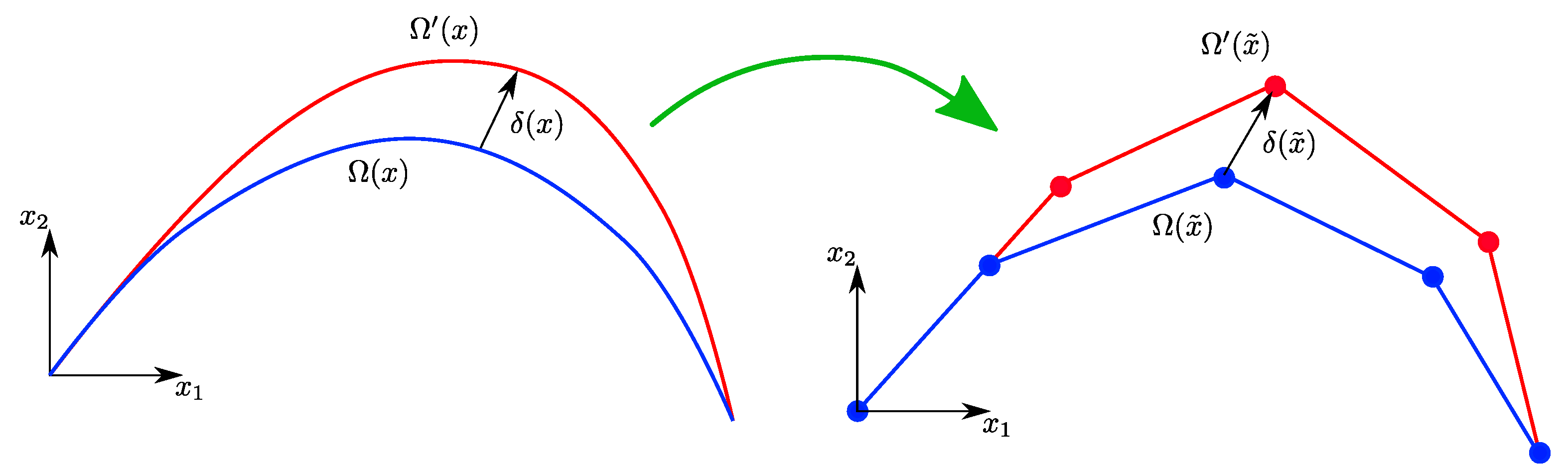
Given the initial ($\mathsf{\Omega }\left(x\right)$) and the final, deformed, surfaces (${\mathsf{\Omega }}^{\prime }\left(x\right)$), the transformation/displacement field that describes the applied modification is simply the distance between the surfaces: $\delta \left(x\right)={\mathsf{\Omega }}^{\prime }\left(x\right)-\mathsf{\Omega }\left(x\right)$, as shown in Figure 1 on the left. Even if the application of this concept is quite trivial, it poses some relevant numerical issues that are strongly related to the structure used to define the surfaces themselves. In the present work, both are described using a mesh-like approach relying on the subdivision surface method characterized by the same element numbers and typology. Consequently, either the discrete form of the initial surface ($\mathsf{\Omega }\left(\tilde{x}\right)$) and that of the deformed one (${\mathsf{\Omega }}^{\prime }\left(\tilde{x}\right)$) are known on a finite set of points $\tilde{x}$ as drawn in Figure 1 on the right. The transformation field $\delta \left(\tilde{x}\right)$ is then known exactly on this set of points.

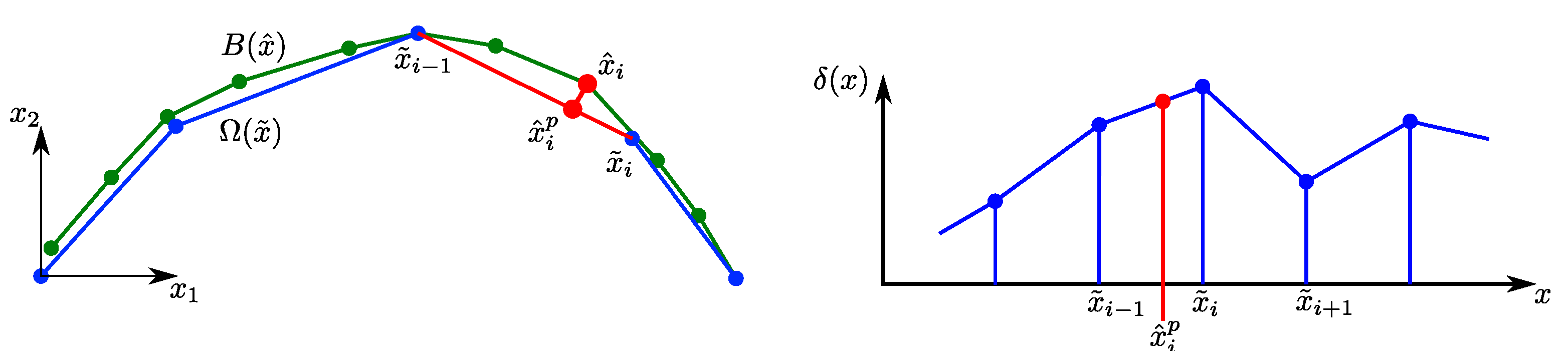
This transformation needs then to be transferred to the surface boundaries of the reference mesh, $B\left(\widehat{x}\right)$, represented by the green lines in Figure 2. These are generally defined by a different set of points ($\widehat{x}$) that typically does not share a consistent space resolution with the initial surface. This is a well known consequence of the meshing process of the initial geometry. Considering the very large number of surface elements and points often used in CFD simulations, this aspect has to be carefully addressed by using a reliable and computationally efficient 3D-space interpolation method. This is realized by a two-step approach. First, each boundary point (${\widehat{x}}_i$)) of the surface mesh of the reference mesh ($B\left(\widehat{x}\right)$) is projected (${{\widehat{x}}_i}^p$) on the initial discrete surface ($\mathsf{\Omega }\left(\tilde{x}\right)$), as shown in Figure 2. The polyhedral face of the initial discrete surface over which the point is projected (the red segment) is stored in a dedicated structure. A 2D interpolation is then carried out. The displacement to be applied to each boundary points ($\widehat{x}$) is computed on the projected points (${\widehat{x}}^p$) by using the weighted distance from the face vertices of the stored face, for which the discrete displacement field ($\delta \left(\tilde{x}\right)$) is available.

The identification of the face corresponding to each boundary point is one of the most demanding steps of the morphing, since it involves thousands or even millions of elements, i.e., all the boundary faces. Thanks to the proposed morphing approach, this operation is required only for the initial discrete surface. So, all the significant geometrical data are calculated and stored once, and then used for any subsequent mesh deformation. The final step of the morphing is the propagation of the displacement field into the volume mesh. To this aim, a simple constrained Laplace equation of the deformation ${\delta }_V$ is solved, following [30]:

$$\nabla ·(\gamma \nabla {\delta }_V)=0$$

(1)

This equation also includes a diffusion coefficient ($\gamma$) that constraints the diffusion in order to increase the solution smoothness and then avoid abrupt variations in the grid deformation. Several formulations of this coefficient have been tested. The best performances of the algorithm were obtained with a quadratic function of the inverse distance from the wall.

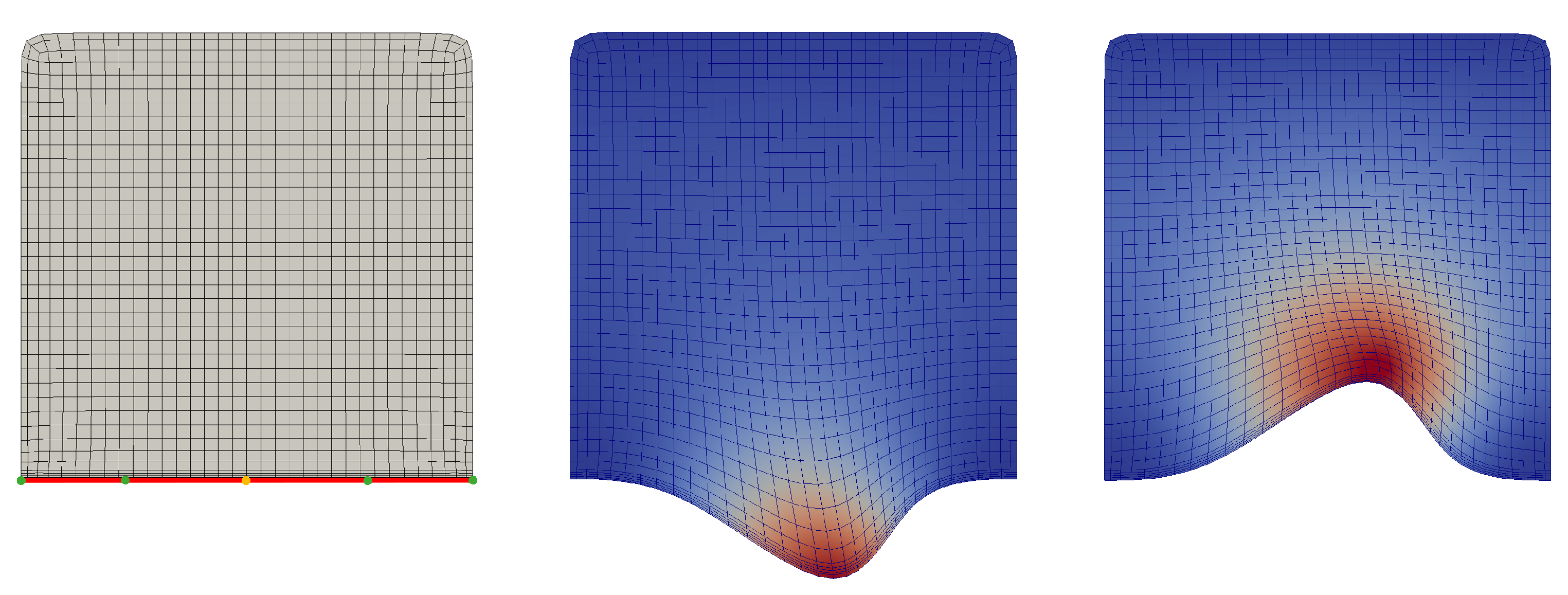
An example of the morphed mesh due to two substantial deformations of the lower boundary (red line) of an initially cubic domain is given in Figure 3, where the internal displacement magnitude (with respect to the initial position of grid points) is monitored by the color contour. The deformation is smoothly propagated throughout the domain and its normal component to the boundary is exactly equal to zero in correspondence of other boundaries where the modification is not applied. This feature is of particular importance when symmetry boundaries are considered because, in this case, their surface points have to move only in the boundary plane itself.

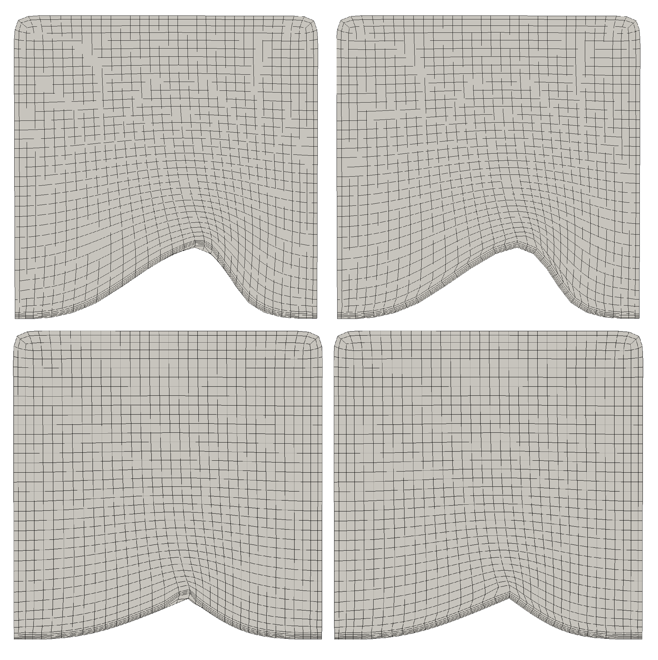
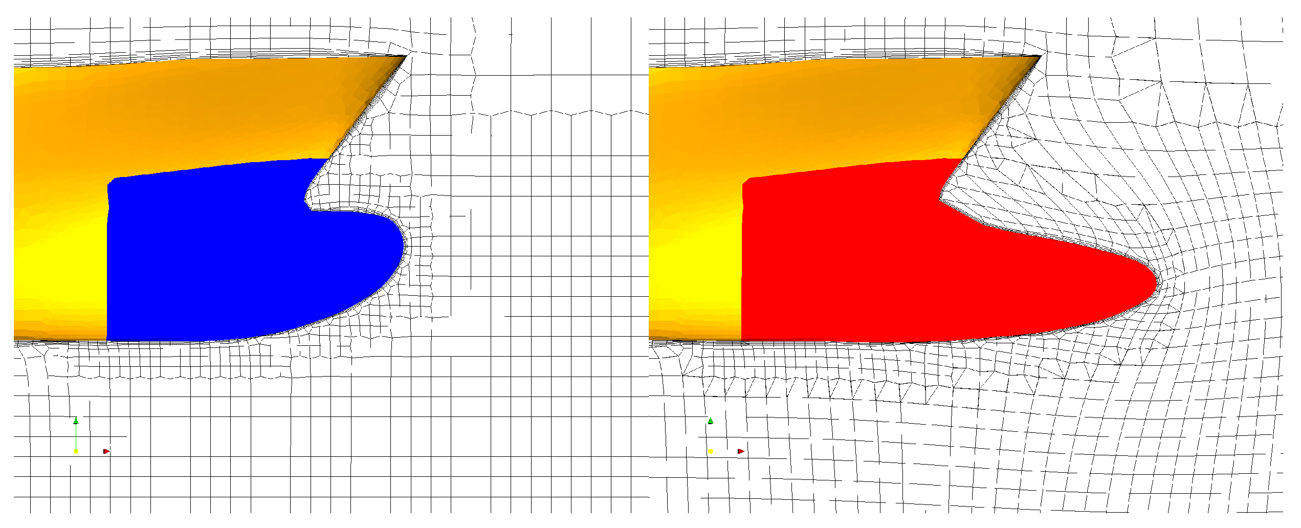
Regardless the application of the quadratic diffusion coefficient that generally provides a high-quality deformed mesh, a certain distortion of the cells can occur especially in correspondence of the wall prism-layer cells, for which the aspect ratio is often critical. An evidence of this possible issue is shown in Figure 4, left side. The prism-layer distortion after the application of the morphing is highlighted for both deformations. This aspect is magnified in correspondence of sharp edges and cusps (in the bottom of the figure) while it generally results in acceptable behavior in case of smoother surfaces (on the top of the figure).

As already highlighted in [31], this is an issue mainly related to the Laplace solver available in the OpenFOAM library. The deformations, computed from their values on the boundaries, are propagated using a cell-centered approach; however, the quantity of interest is the displacement on the vertices, as such, a space interpolation procedure is applied. Such a propagation/interpolation might generate unwanted mesh distortions that ultimately alter the quality of the morphing especially in the prism-layer region, where the grid is designed to accurately model the boundary layer. The prism-layer cells are re-generated based on a re-distribution of the morphing displacement on all the prism-layer cells, accordingly to the deformation applied to the wall. Therefore, it imposes the same deformation on the internal boundary cells equal to the corresponding boundary point (the nearest point on the wall connected with the internal one). This technique, even if might create slightly less regular cells at the outer boundary of the prism layer mesh, completely recovers the arrangements of cells close to the walls, as shown in Figure 4, right column.

Figure 5 shows an example of the mesh deformation procedure applied to a more complex shape, i.e., a hull bulbous bow (this shape, incidentally, is the one adopted in the next section where more details can be found). The mesh deformation in proximity of the bulbous bow is well-visible, showing regular, high-quality cells even when large deformations are considered. Compared to the initial arrangement, the prism-layer correction maintains a good shape of the prisms cells, also in the highly distorted zones, proving the applicability of the developed morphing approach. This morphing approach requires a fraction of the time needed for a completely new mesh, which makes clear the benefits in the case of automatic optimization processes. Considering the computational efficiency, the data extraction (i.e., the interpolation weights and face/point correspondence) from the initial surfaces and the reference mesh is the most expensive step. This requires about 25% of the whole CPU time used to generate a completely new mesh from scratch, as highlighted in

Table 1. Comparison of the CPU time between the proposed mesh deformation procedure and the mesh generation.

Procedure	CPU Time
Mesh generation/re-meshing of each case	100%
Data extraction (initial surface/mesh only)	25%
Mesh morphing	12%

by using a typical surface/mesh arrangement on the reference case. This operation, even if quite expensive, is required only once on the initial geometry. The calculation of the displacement field is almost instantaneous and its propagation, i.e., the solution of the Laplace equation using the OpenFOAM libraries, is faster than the complete re-meshing of the case of about an order of magnitude. This makes the proposed morphing approach a cost-effective method able to keep comparable grid quality parameters over shape deformations. In addition, this morphing method maintains a direct correspondence between points belonging to the initial and the deformed meshes. This can reduce the possible uncertainty of the CFD solutions introduced by using different mesh arrangements, particularly if small variations are under investigation.

3. Optimization Framework

When an optimization process is used, the overall workload is intrinsically related to the computational effort required for each design evaluation. When a high-fidelity solver is used, the overall cost can be not affordable for the design procedure to be applied at an industrial design level. This risk is further increased if a highly multi-dimensional design space (i.e., several design parameters) needs to be considered to explore unconventional design solutions (those that usually provide the highest improvements) since the number of evaluations required for a decent convergence to optimal solutions exponentially increases.

Often, to overcome these issues, a surrogate model is used to reduce the computational time. Starting from a limited number of sampled points in the design space, fully characterized in terms of key performance indicators by the high-fidelity solver, it approximates the behavior of the objective function everywhere in design space using polynomial interpolations, radial basis functions, neural network or Gaussian processes. By exploiting this “black box”, the optimization can be performed substituting the real evaluations of the performance of a certain configuration with its approximation using this new implicit function, making the computational effort negligible if compared to the computational time associated to the high-fidelity solution.

In the subsequent subsections each method adopted to define and morph the surface and to evaluate the response values are reported and briefly discussed.

3.1. Surface Definition and Deformation

The first issue of a completely automated process that requires the evaluation of many different design configurations by a CFD flow solver concerns the realization, each time the design parameters are varied, of a robust (i.e., watertight) representation of the geometry to be used from the grid generation to the post-processing of results. Several approaches can be adopted to address this problem. Each should be able to represent complex shapes, such as the ship hull, characterized by smooth and faired surfaces as well as by flat or surfaces with sharp edges. In current work, the approach previously proposed in [32,33] is employed. It is based on the combination of a subdivision surface (SS) method, suitable to describe the hull surface by means of a control polygon, and a free-form deformation (FFD) technique suitable, instead, to reduce the number of design parameters of the optimization process.

The subdivision surface method, contrarily to the widely used B-surf-like techniques (B-spline surfaces), adopts a flexible control polygon made of an unstructured mesh; therefore, it allows us to easily change the local control polygon resolution, ensuring that all the control polygon geometrical properties are directly transferred to the final surface. The SS approach basic idea consists of hierarchically splitting a control polygon (seen as a polyhedral surface mesh) and rearranging the old and new points by means of weighting functions able to generate a smooth limit surface (theoretically achieved after an infinite number of subdivisions).

This technique was first proposed by Chatmul–Clark [34] in the context of computer graphic. Its generality and equation-free foundation make it a helpful tool in the marine field, where quite complex geometries (not definable by simple equations) need to be managed. The current approach is based on the Quad/Tri method [35,36] where the classical Chatmul–Clark algorithm (limit surface made of only quadrilateral faces) is combined with algorithm by Loop [37] (limit surface made only of triangular faces) using a blended approach for the interface regions. 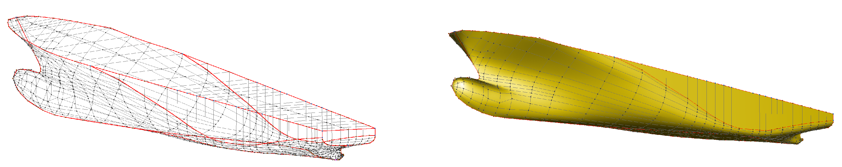This method generally guarantees a $C^2$ limit surface everywhere except in correspondence on the extraordinary points, where the algorithm is downgraded to a $C^1$ limit surface. In addition, it can easily manage also crease edges and vertex points to represent, respectively, sharp edges and cusps typical of many ship types as for instance high-speed planning hulls. An in-house developed code controls the whole geometry generation that is currently presented for the DTC hull, which is the test case selected to assess the reliability of the entire process ( details can be found in Section 4), from geometry parametrization to hull shape optimization. The control polygon of the subdivision surface is shown on the left of Figure 6. Grey lines represent the internal edges of the faces used for the smoothing of the limit surface; red lines, instead, show the user-defined creases: those at the side–bridge intersection and those that identify the trace of the longitudinal symmetry plane. The limit surface (that after four subdivision steps) is shown in yellow on the right of the same figure and the unstructured nature of the subdivision surface description is well visible in the more refined polygon adopted locally to describe the bulbous bow.

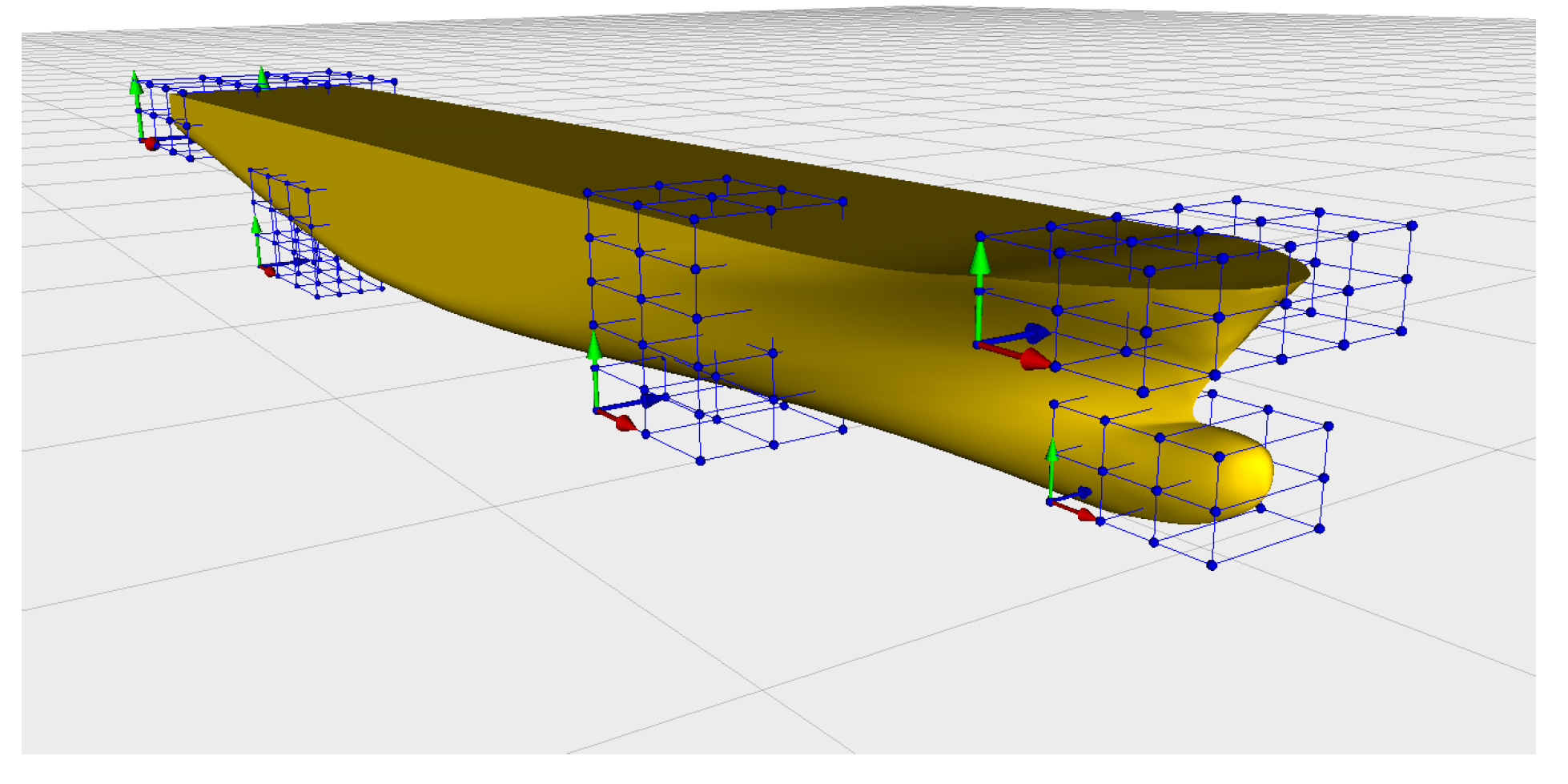
Even if a surface deformation can be easily obtained by a direct modification of the control polygon (using subdivision surfaces a smooth and watertight surface is always obtained, also after the alteration of a single point of the polygon itself), the number of free parameters (in the case of Figure 6 more than 400 control points) will be prohibitive to be managed in an optimization process. In addition, moving a single point determines a very local deformation while, often, relatively global variations of the hull shape are preferred. For this reason, a free-form deformation [38] approach has been considered to deform globally and locally the hull shape. Figure 7, for instance, shows possible FFD zones (the blue FF polygons applied to the surface of the hull) encompassing both large portions of the hull as well as local details such as the stern or the bow, realizable with the developed tool; however, rather than modifying directly the points of the subdivision surface, the FFD is applied to its control polygon through which the surface is reconstructed each time. This permits a more reliable and easy handling of the deformation, as presented in [32,39].

3.2. Flow Solver

The optimization process always requires a solver to evaluate the objective functions of all the configurations iteratively selected towards convergence. In the context of the hydrodynamic shape optimization of hulls, the minimization of the ship resistance is the simplest and the more obvious design objective to be adopted for the design. Its evaluation can be carried out employing different flow solvers, from simple potential flow codes to accurate high-fidelity solvers based on RANS equations. Further, in the current work, the design objective of the design by optimization process, aimed at showing the potentialities and the flexibility of the mesh morphing approach, is the minimization of the ship resistance that has been computed using the open OpenFOAM CFD library [17], the same that has been already used to handle portions of the mesh morphing process. OpenFOAM is a CFD package, based on the finite volume approach, that includes several tools designed to manage flow simulations from the pre- to the post-process phase. It solves the classical Navier–Stokes equations rearranged, for current activities, considering the Reynolds decomposition to account for the turbulent effects on the mean flow quantities through the $k-\omega$ two-equation turbulence model. Considering the presence of a two-fluid problem (air and water) an homogeneous mixture approach is considered and solved using the volume of fluid (VoF) method. 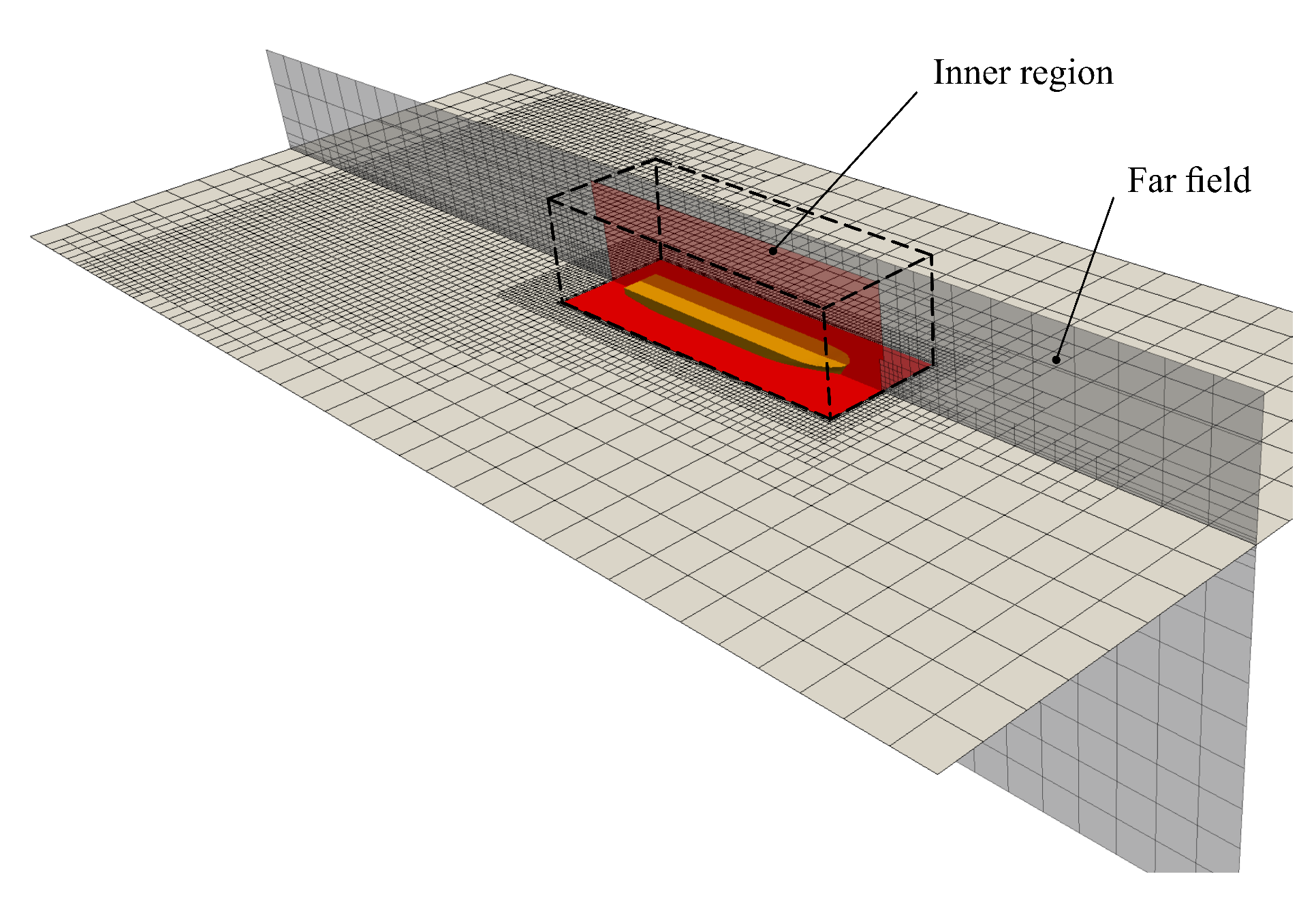OpenFOAM handles unstructured meshes with arbitrary (polyhedral) cell shapes. The particular nature of the flow under investigation suggests the use of hexa-dominant cells with special refinements aimed at capturing the peculiarities of the flow around ship hulls such as the wave pattern. To this aim the computational grid is realized by a combination of two subdomains, a far-field and an inner region surrounding the hull, where different tools and meshing strategies are adopted. This mesh arrangement has been already successfully adopted in [40,41]. A sketch is reported in Figure 8.

In the far-field (grey region), the mesh has been generated using the BlockMesh tool, which is the basic meshing tool available in OpenFOAM. It provides several features to create (simple) fully hexa grids with concentric and anisotropic refinements in correspondence to the free surface. These are of particular importance since they allow to accurately compute the wave pattern avoiding spurious oscillations (usually related to cell dimension variations across the free surface), limiting at the same time the overall cell count and the required computational effort. The mesh of inner region (red region in the figure), instead, is realized using the cfMesh library [42]. It generally provides an higher flexibility in case of complex geometries, in particular for what concern the realization of prism layer cells (Y+ less than 150 in current case), ensuring hexa-dominant cells arrangements having a quality adequate for the successful application of the mesh morphing. The final arrangement, considering the volumetric refinements close to the hull and those inside the Kelvin angle visible in Figure 8, consists of about 0.8 million cells.

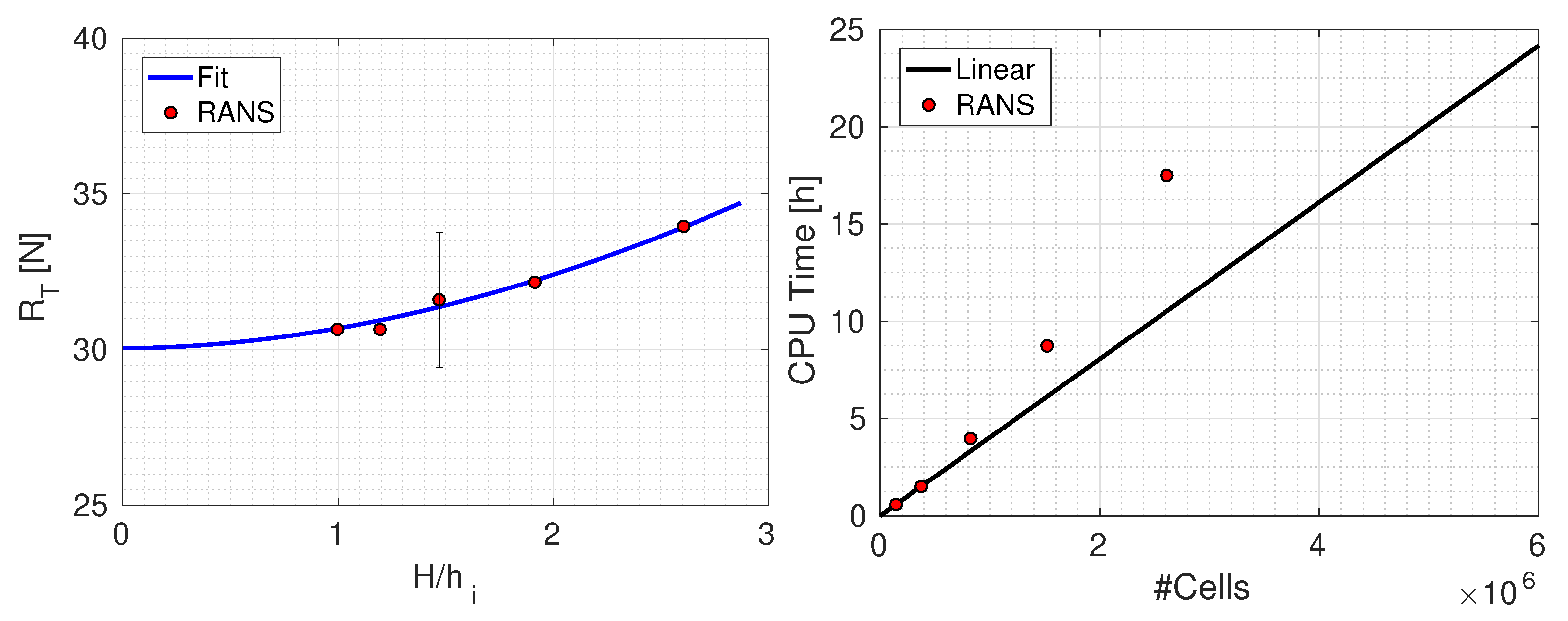
This reference mesh arrangement has been rationally selected after a dedicated mesh sensitivity analysis that involved five different grids ranging from 0.14 to 2.6 Million cells. They were obtained varying the far-field cell size, for corresponding computational time (on a 24 cores, 2.4 GHz workstation) ranging between half to 18 h, as summarized in

Table 2. Mesh sensitivity analysis. Reference DTC hull at Froude = 0.218. CPU time evaluated on an Intel 2.4 GHz/64Gb Workstation with 24 cores.

Mesh	Cell Number	Drag Resistance [N]	CPU Time [h]	Error
Extrapolated	∞	30.042	-	-
1	2.62M	30.814	17.50	2.57%
2	1.52M	30.650	8.71	2.02%
3	0.82M	31.602	3.98	5.19%
4	0.37M	32.161	1.53	7.05%
5	0.14M	33.951	0.60	13.01%

. The selection of the best accuracy/computational effort balanced configuration is, indeed, mandatory for the practical application of an optimization-based design procedure, especially in the case of using high-fidelity RANS solvers, whose computational efficiency in these kinds of contexts is questionable. Moreover, any optimization process is based on the relative merits of one configuration with respect to the others, making the absolute accuracy less relevant than the uncertainty of the calculation to drive the process to convergence. A recent paper [39] highlighted exactly this aspect, since it showed for a very similar ship optimization problem that the relative performance differences among several hull shapes remained almost unchanged (at least in terms of their ranking) even if a quite coarse grid is adopted for the analyses. Using the proposed coarse grid, then, is reasonable to be adopted to drive the optimization loop. Then, as in best practices in this field, a finer mesh could be used to validate the final optimized design.

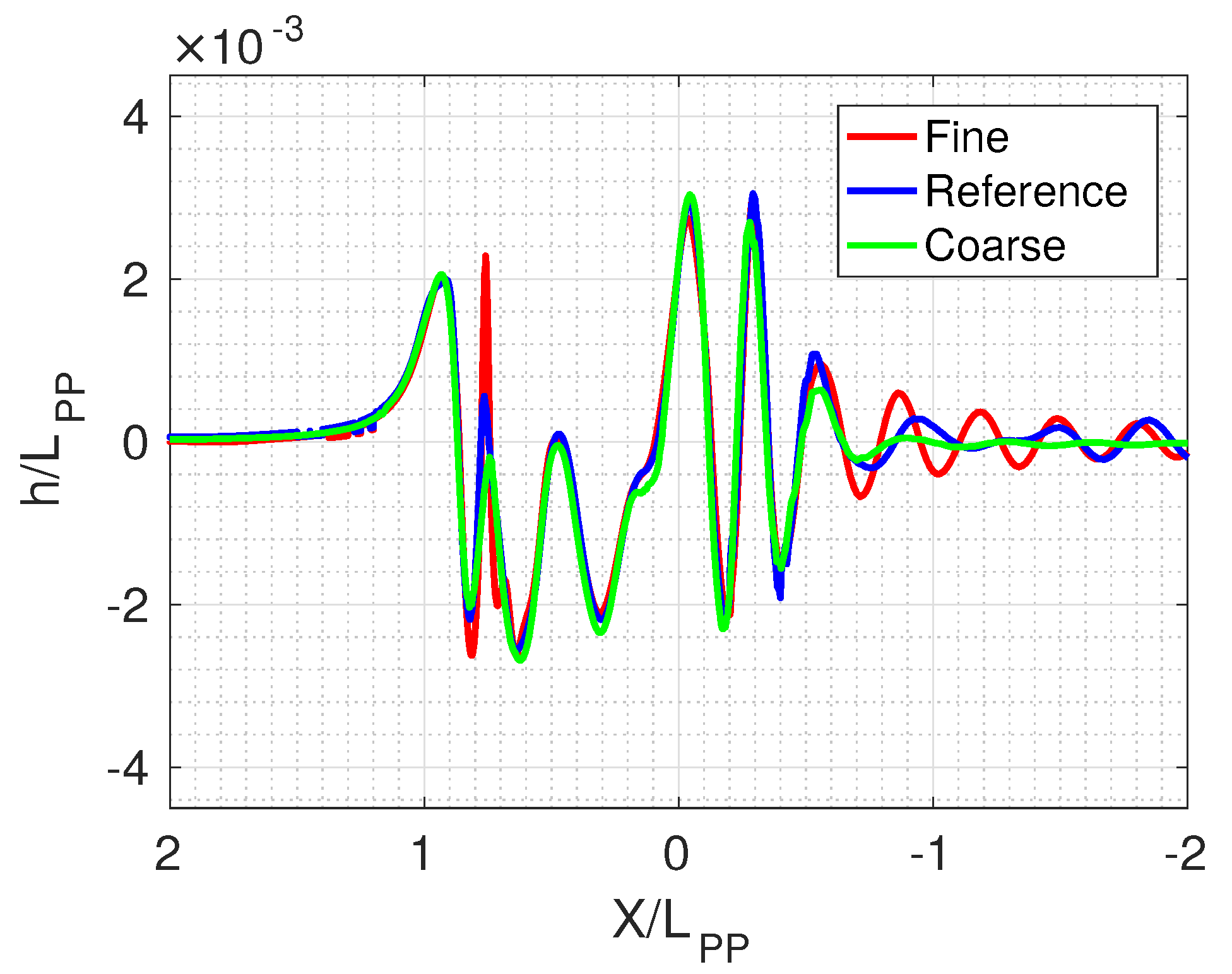
The sensitivity analysis described in Figure 9 shows, exactly, a good convergence trend of the results with the number of cells. Compared to the extrapolated value, evaluated using the methodology proposed by [43], differences are about 2% for the finest (2.6 million cells) and increase to more than 10% for the coarsest case. The reference mesh of 0.8 million elements has a difference of about 5% but represents a decent compromise in terms of computational effort for all the calculations needed in the optimization process since, as expected, the computational time increases significantly more than linearly moving to more refined configurations. Wave profiles (sampled on the hull and on the symmetry plane) of Figure 10 confirm this trend too. With the exception of the second wave peak from bow (about at $x/L_{PP}=+0.8$), in correspondence of which some differences of the wave profiles especially for very coarse meshes can be appreciated, the wave field is very similarly predicted. A negligible phase shift is observable in the far field between the reference and the finest grid, while the numerical damping associated to an excessively low spatial resolution, prevents the formation of waves in the case of the coarsest mesh. Compared to the model scale towing tank measurements of

Table 3. EFD and CFD comparison of the DTC hull resistance at different Froude numbers.

${\mathit{F}}_{\mathit{N}}$	EFD Data [N]	CFD Data [N]	Error
0.192	24.14	23.84	−1.24%
0.209	28.99	28.99	−0.02%
0.218	31.83	31.60	−0.72%

, available in [44], current results show a very good agreement with discrepancies, in the range of Froude number between 0.192 and 0.218, around 1%. Combined with the results collected by Islam and Soares [45], that by systematically analyzing different hulls using the same flow solver and very similar grid arrangements evidenced comparable results, both in terms of computational accuracy and uncertainty, the numerical setup selected for current analyses seems definitely adequate, also having in mind the scope of the optimization, which is testing the flexibility of the developed pre-processing approach based on the mesh morphing included in a fully automated framework.

3.3. Surrogate Model

Even if the computational time is kept as low as possible by the selection of the most efficient computational setup, high-fidelity RANS solvers do not provide the sufficient efficiency to be applied with success in an optimization design process. To overcome this issue, accurately trained surrogate models, as already proposed in [46,47,48,49,50], can substitute the high-fidelity solver to make the process applicable also at an industrial, time constrained, level. In current analyses, a Gaussian process (GP) based on the ordinary kriging method has been applied as surrogate model. Kriging is a method for the interpolation/approximation of experiments based on the computation of the prior covariance of the available data. The value of a function at a given point is a weighted average of the known values of the functions in the neighborhood of the point itself. This weighted average is realized by a combination of a regression (or trend) function constructed based on the data and a Gaussian process built through the residuals between the trend function and the data themselves. In the ordinary kriging, as the one adopted in current analyses, the regression function is an unknown constant while the characteristics (mean and standard deviation) of the Gaussian process are calculated by the minimization of the likelihood function that measures the goodness of fit of a statistical model to the samples of given data. Among the possible formulations, detailed in [51,52], the interpolation method has been preferred in order to exactly reconstruct the computed values in correspondence of the sampled points in the design space.

4. Application

The proposed approach, from pre-processing to optimization using the surrogate models, has been applied to the the Duisburg test case (DTC) hull. The DTC is a Post-Panamax, 14000TEU, single-screw container vessel designed for numerical and experimental benchmarks at the Institute of Ship Technology, Ocean Engineering and Transport Systems (ISMT) in 2012 [44]. Model scale tests (scale factor of 1:59.407) were performed at the model test basins SVA Potsdam for resistance and propulsion tests. The availability of geometry and measurements made this hull a quite largely adopted test case in the research community especially for the validation of numerical analyses, with particular attention to energy saving since the ship is equipped with a twisted rudder with a Costa Bulb.

The ship, as evident from the body plan of Figure 11, is characterized by a pronounced bulbous bow, whose shape is the object of the proposed hydrodynamic optimization regardless the design functioning condition of the ship. The main data of the ship are reported in

Table 4. Main dimensions and data of the DTC hull. Full and model scale.

Parameter	Full Scale	Model Scale
$L_{BP}$ [m]	355	5.976
$B_{WL}$ [m]	51	0.859
$T_{Design}$ [m]	14.5	0.244
Sink and Trim	Even keel	Even keel
Volume [m${}^3$]	173,467	0.827
$C_B$ [-]	0.661	0.661
$S_W$ [m${}^2$]	22,032	6.243
$V_S$ [kn]	25	3.244

. At full scale, indeed, the ship operates at a speed of about 25 knots, equivalent to a Froude number of 0.217. At this speed, most of the ship resistance is due to friction and only a fraction to wave resistance, which instead is the contribution to the total resistance that can be modified (i.e., minimized) by a shape variation of the bulbous bow. This poses possible issues in terms of efficacy (and opportunity) of the optimization process, but it takes nothing away from the possibility to stress the automation process that encompass subdivision surfaces, free-form deformations, mesh morphing, CFD solution and post-processing compared to a more “global” modification of the hull. When the entire hull dimensions and shape are varied, indeed, several additional considerations (and constraints) different from pure hydrodynamic aspects have to be addressed. A global modification of the hull geometry influences the structural layout or the payload distribution, with obvious consequences on hydrostatics, requiring in the end a much more complex and multidisciplinary design environment for fair comparisons between the reference and the optimal configurations. A local modification of the bulbous bow, instead, only negligibly changes the global characteristics of the ship, legitimizing the simplified optimization process (minimization of resistance) adopted for the current study.

Figure 12 shows the used FFD box, arranged around the bulbous bow of the reference DTC geometry. Regardless of the simplified shape of the FFD polygon, in principle a total of 18 free parameters could be used to alter the shape of the bulb surface by changing the collocations of the control points of the corresponding subdivision surface polygon. To further reduce the complexity of the design, the design parameters were reduced to only two by combining and joining the “degree of freedom” of the FFD points. Only the six green dots of the foremost plane are moved all together along two directions (longitudinal and vertical). The first parameter ($F_1$) controls the transformation of the bulb length, the second ($F_2$) is used to vertically move its nose.

The range of variations of the design parameters made non-dimensional with respect to the length between perpendiculars are reported in

Table 5. Range of variations of the design parameter.

Parameter	Minimum Value	Maximum Value
$F_1[\%L_{BP}]$	−3.35	6.69
$F_2[\%L_{BP}]$	−4.18	0

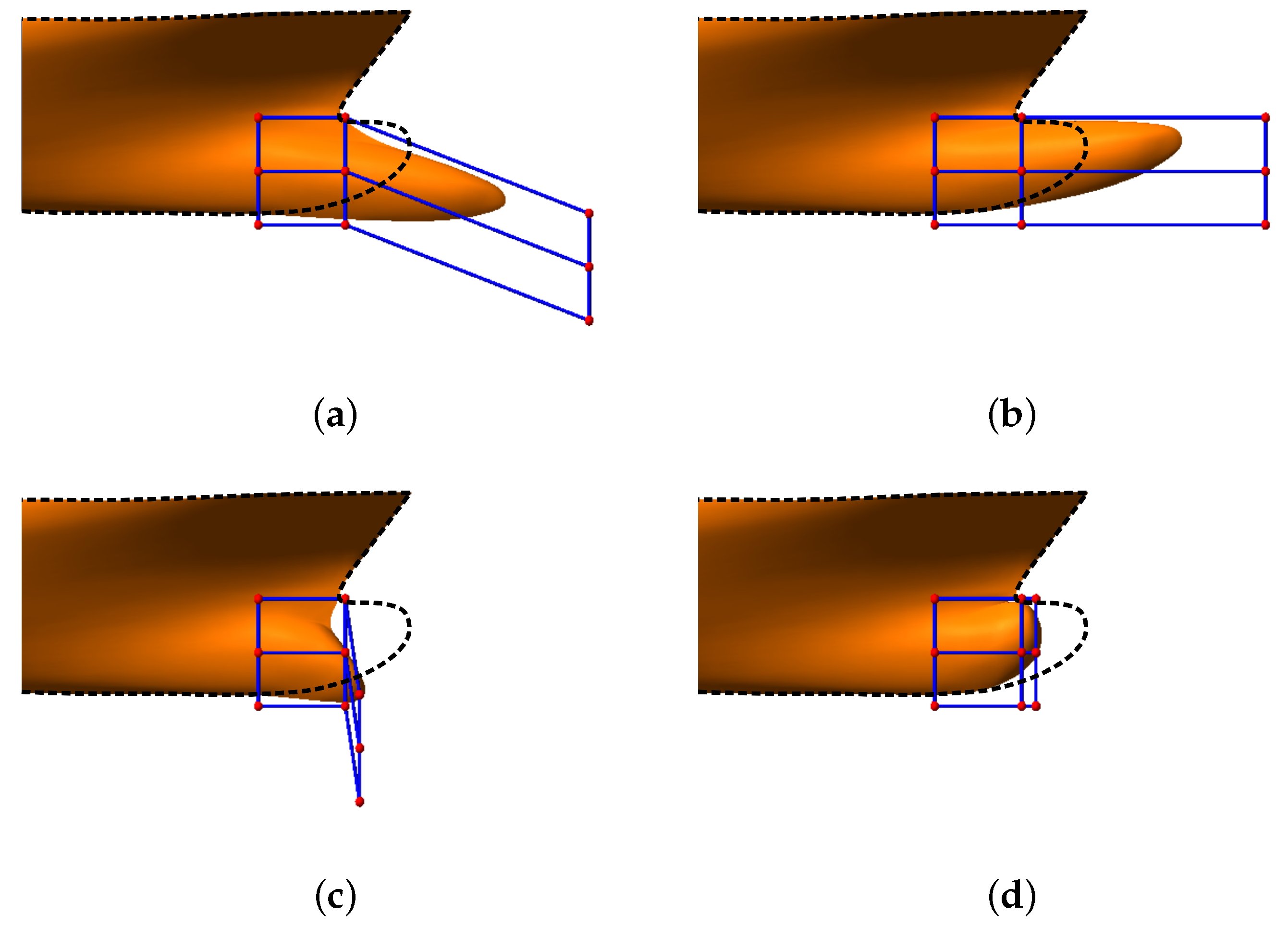
. Figure 13 compares the original bulbous bow with the possible hull bow shapes allowed by these ranges, in particular those in correspondence of the maximum/minimum values. With respect to traditional guidelines for the design of bulbous bows, the resulting geometries have a certain unconventional nature that is exactly functional to the scope of the work: to stress the mesh morphing approach with shapes far from the reference surface (and mesh) with the aim of accurately exploring wider design spaces where an improvements of performances is easier.

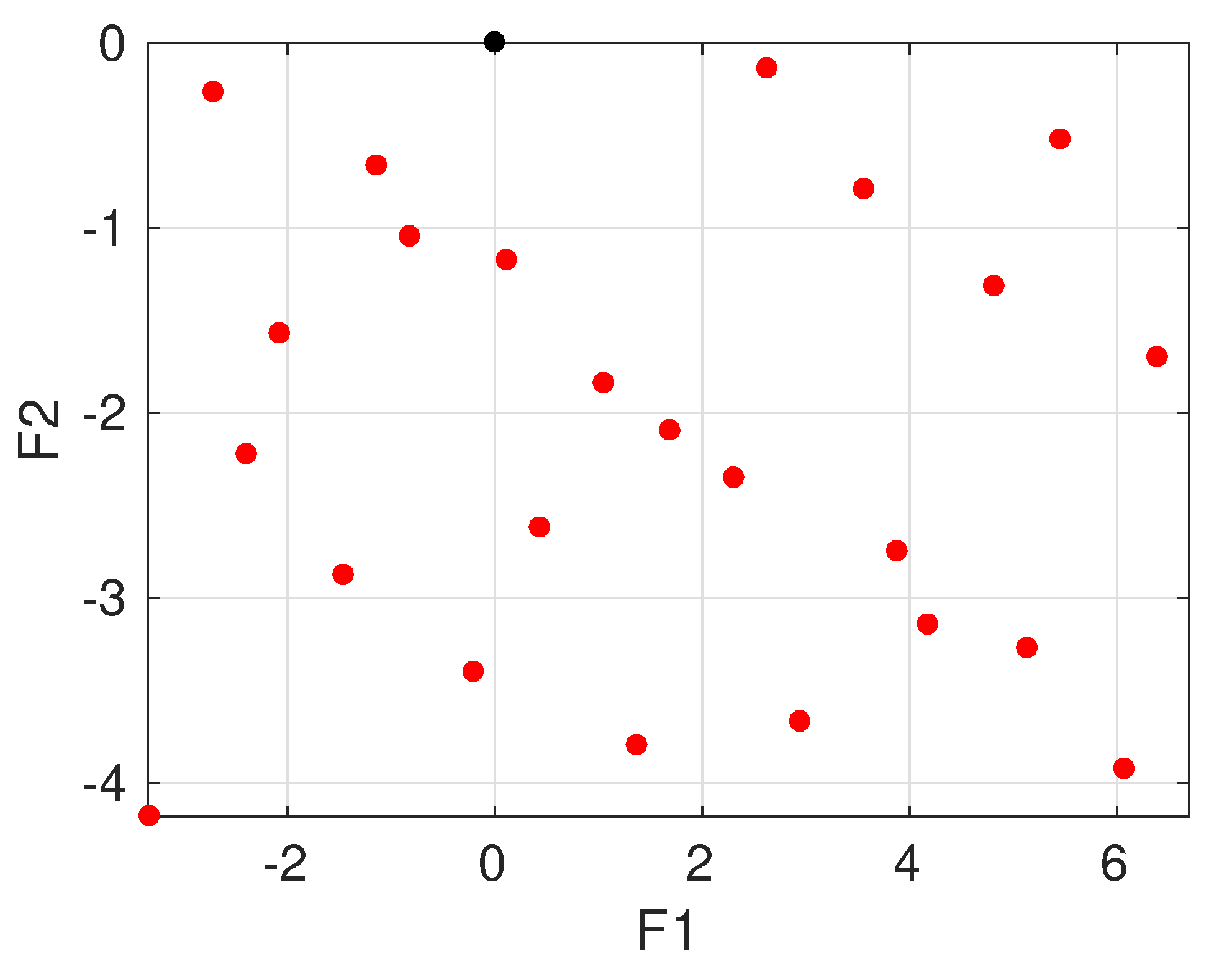
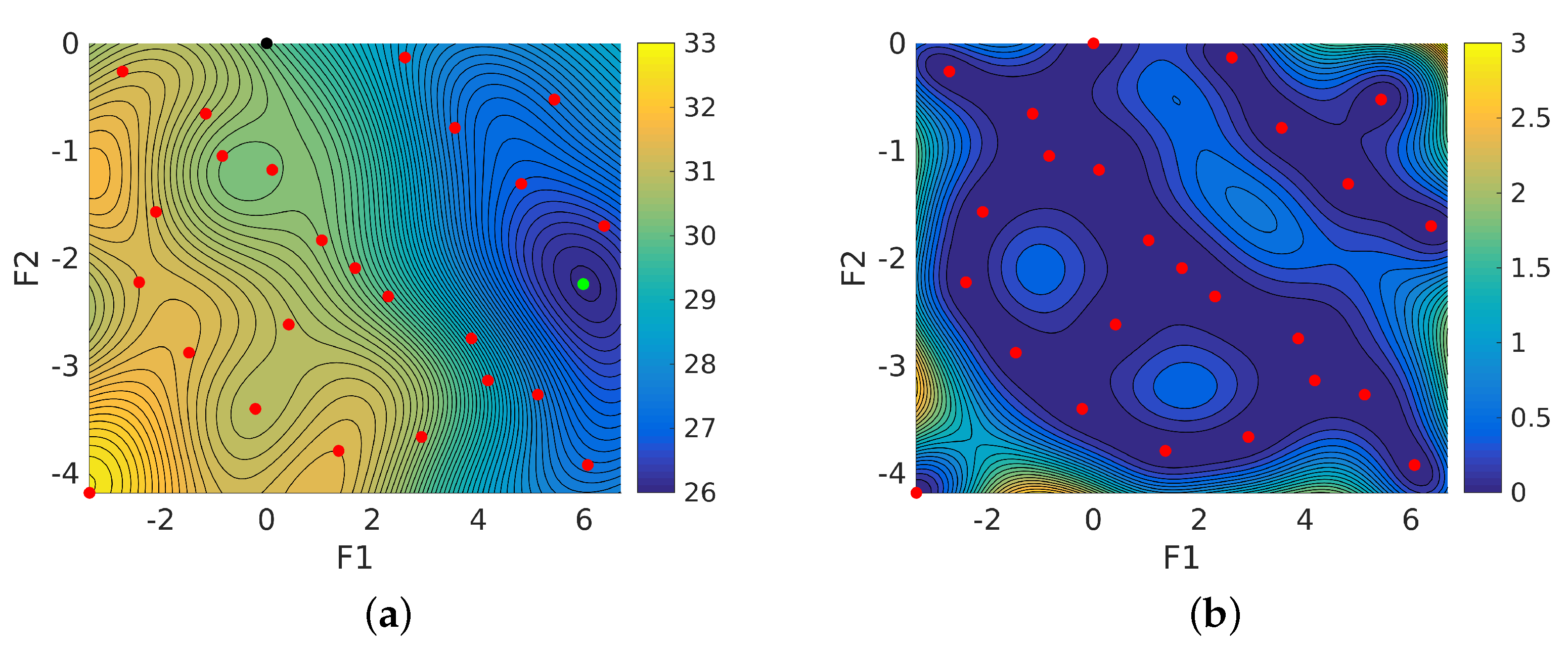
The initial exploration used to train the kriging metamodel was realized by sampling the two-dimensional design space of Figure 14 with 25 configurations selected using the Sobol spacing [53]. These designs also include the reference hull, identified by both the $F_1$ and $F_2$ design parameters equal to zero. Each geometry was obtained by a modification of the hull surfaces using the FFD. The corresponding computational grid was realized only by morphing the mesh of the reference hull and its performance (i.e., resistance) was collected by a CFD analysis carried out using the models introduced in previous section. The relationship between the bulb shape (monitored by the two design parameters) and the total ship resistance is summarized in Figure 15, where the interpolating surface was built using the surrogate model. Regardless the small number of sampling point in the design space, some clear and credible trends can be understood from the data. Resistance is inversely proportional to the bulbous bow length (the $F_1$ parameter) but also a certain preference for bulbous noses shifted down can be appreciated.

Even if the sampling of the design space is not the final one for an accurate optimization process based on metamodels, and some additional configurations could be added to better characterize the behavior of the resistance at first where the estimated uncertainty of the model is higher, the reliability of the model seems sufficient for a preliminary design process. The maximum uncertainty in the design space, indeed, is lower than 3% with the mean square error associated to the leave-one-out procedure of 2.59%. In this design space the total resistance variation is higher than 23%, showing that there are margins for an improvement of the performances of the reference hull through the optimization. Only by using the surrogate model, the design by optimization identifies in the parameters $F_1=5.983$ and $F_2=-2.239$ the geometry capable of reducing to 26.17 N (−13%) the drag of the DTC model. Direct RANS calculations predict for this hull a resistance of 26.59 N, then about 10% lower than the reference. This improvement is significantly better than the numerical uncertainty associated with the adopted computational mesh, which was estimated of about 6% in the calculations of Figure 9, proving the effectiveness of the proposed approach.

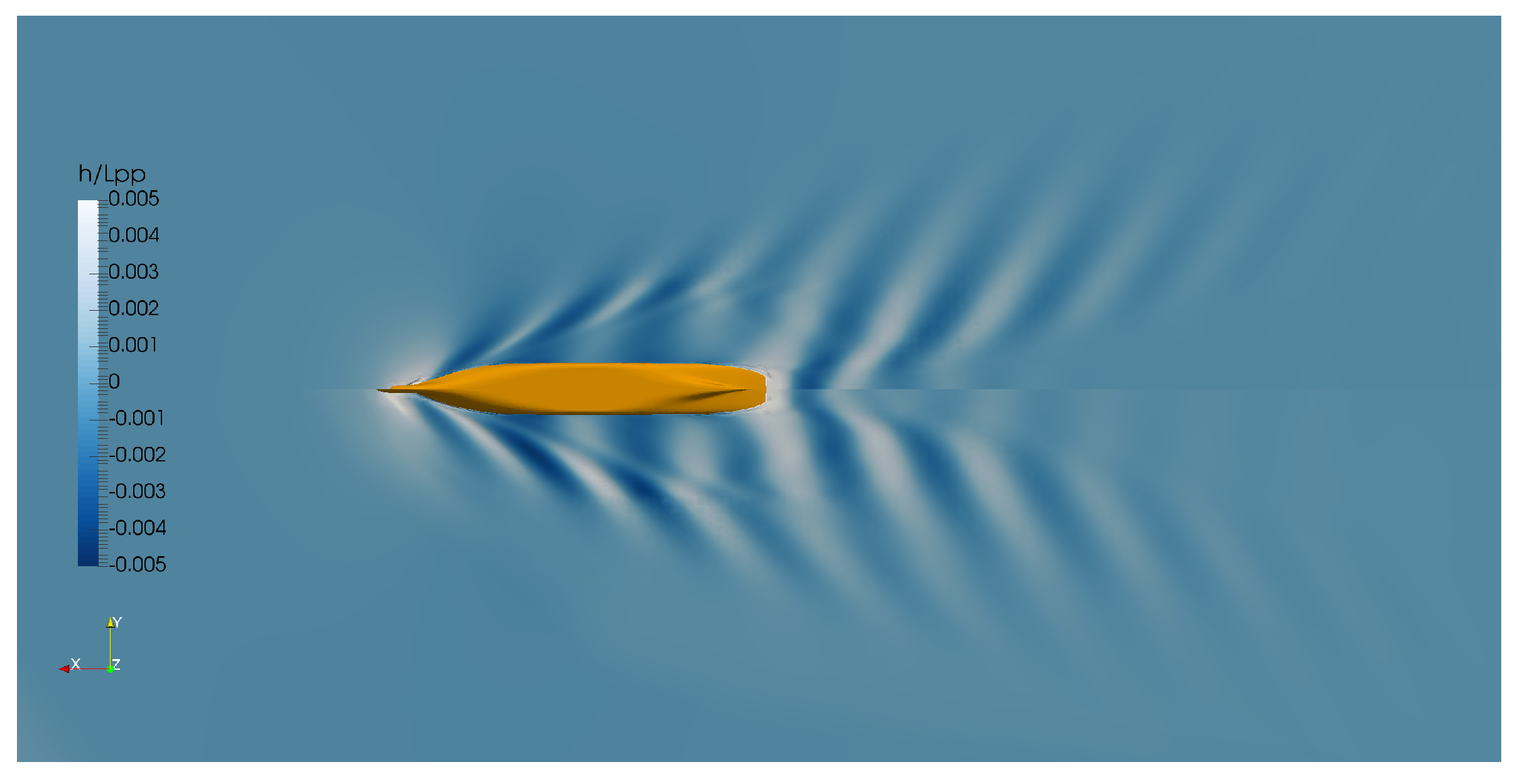
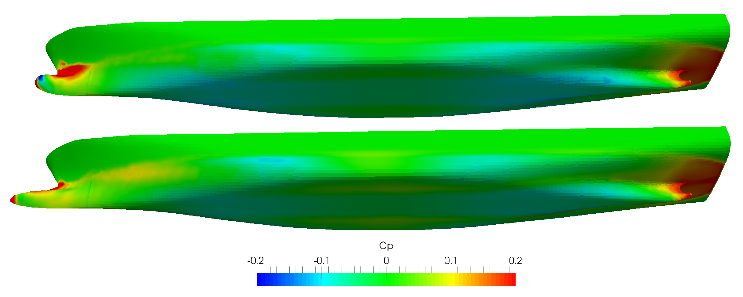
Reasons for this substantial reduction are visible in Figure 16 and Figure 17 where the initial and the optimized hulls are compared in terms of wave fields and dynamic pressure distributions. The longer bulbous bow of the optimized geometry changes the spatial position of the firs wave crest, inducing in turn a different interference between the bow and stern waves. Further, the reduction of the pressure peak on the bow (and the corresponding increase in the recovery pressure on the stern) of the optimized hull contributes to the overall improvement of the ship performances.

5. Conclusions

A mesh morphing method has been developed and embedded into an hydrodynamic design by optimization process to reduce the overall computational effort by avoiding the re-meshing of each new configuration, and to improve the flexibility of the entire process in the light of fully automated, unsupervised design activities. These results have been achieved by an appropriate combinations of techniques. In particular, subdivision surfaces and free-form deformations have been used to handle the surface generation and modification. The OpenFOAM Laplace solver and a prism layers regularization approach have been applied to propagate the surface deformation inside the computational domain, while the blockMesh and the cfMesh libraries allowed for the generation of the initial unmorphed high-quality volume grid.

The whole process was then tested on a benchmark case, i.e., the DTC hull. The bulbous bow shape has been modified by using a 2-dimensional design space wide enough to stress the morphing approach in order to assess the flexibility of the developed pre-processing method in case of complex, relevant, shape variations.

A surrogate model based on the kriging interpolation has been used to drive the design process, requiring the evaluation of 25 different configurations to train the metamodel and use it in the optimization.

A substantial reduction of the total ship resistance, predicted at first by the surrogate model and confirmed in the end by a dedicated CFD analysis, has been achieved then confirming the reliability of the proposed design framework.