
CPM-OFDM Performance over Underwater Acoustic Channels


1
Department of Computer Engineering, Umm Al-Qura University, Makkah 21955, Saudi Arabia
2
Telecommunication Engineering School, University of Malaga, 29071 Malaga, Spain
3
Institute of Oceanic Engineering Research, University of Malaga, 29071 Malaga, Spain
*
Author to whom correspondence should be addressed.
J. Mar. Sci. Eng. 2021, 9(10), 1104; https://doi.org/10.3390/jmse9101104
Submission received: 8 September 2021
/
Revised: 27 September 2021
/
Accepted: 1 October 2021
/
Published: 11 October 2021
(This article belongs to the Section Physical Oceanography)
Abstract
:We propose and evaluate the performance of a continuous phase modulation based orthogonal frequency division multiplexing (CPM-OFDM) transceiver for underwater acoustic communication (UAC). In the proposed technique, the mapper in traditional OFDM is replaced by CPM while a realistic model of underwater channel is employed. Bit error rate (BER) as well as peak to average power ratio (PAPR) performance of the proposed scheme is evaluated using Monte-Carlo simulations. The error performance observed clearly establishes the superiority of CPM-OFDM over traditional OFDM schemes. Specifically, a value of 7/16 or 9/16 for the modulation index gives the best error performance. Furthermore, the error performance of the proposed scheme is within acceptable values up to a transmitter–receiver distance of 1.5 km. Additionally, the PAPR performance of the proposed scheme suggests that like other OFDM schemes, a PAPR reduction scheme is mandatory for acceptable PAPR performance of CPM-OFDM.
1. Introduction
The underwater acoustic channel is considered one of the most complex channels [1], having a fairly long delay spread that causes frequency selectivity due to multiple paths and time selectivity due to Doppler effect. Thus, single carrier and multicarrier acoustic communication systems experience inter-symbol interference (ISI) and inter-carrier interference (ICI), respectively. Further, acoustic transmission generally utilizes lower frequencies and the bandwidth is extremely limited [2]. This makes the channel wideband in nature as the bandwidth is not negligible compared to the center frequency. Traditionally, single carrier techniques have been used for underwater data transmission but the increasing complexity of the equalization schemes limits their ability to achieve higher data rates [3].
OFDM has reliably been used in multicarrier underwater acoustic communication (UAC) systems where high data rate transmission over longer distances is required [4]. It can effectively counter ISI by dividing the bandwidth into smaller overlapping subcarriers that are orthogonal to each other, producing a longer symbol duration [5]. This also simplifies the equalization scheme to a greater degree. Since there is a demand for higher data rates in future underwater acoustic systems, it will cause the symbol duration to become shorter and shorter. This will increase the complexity of equalization [6]. OFDM not only offers higher data rates, it also reduces the complexity of the equalizer to just one tap. Furthermore, the equalization is carried out in the frequency domain and the fast Fourier transform (FFT) in the receiver reduces the equalizer complexity even further [7]. However, the orthogonality of the subcarriers of an OFDM system is severely affected by Doppler shifts due to variations in phase.
Continuous phase modulation (CPM) and continuous phase frequency shift keying (CPFSK) have been employed in communication systems for more than four decades [8]. The main advantages of these schemes are that the signal is power and spectrum efficient, has a constant envelope, has less out of band radiation, and possesses phase continuity [9,10,11]. Traditional OFDM systems use memoryless modulation schemes such as PSK and QAM in the mapper. Very limited work has been done incorporating CPM in the mapper of an OFDM system. In this work, we evaluate the performance of a typical CPM-OFDM system over doubly-selective underwater acoustic (UWA) channels [4,12]. The main contributions of this work are as follows:
- An overview of the work done on CPM-OFDM and similar schemes (presented in this section).
- Design of a CPM-OFDM transceiver for low bandwidth and doubly-selective UWA channel.
- Performance evaluation of the proposed transceiver over the UWA channel using computer simulations. Specifically, we present:
- o
- Bit error rate vs. SNR plots for various rational values of the modulation indices and identification and analysis of good performing indices.
- o
- Bit error rate vs. SNR plots for varying transmitter-receiver distances and a discussion of the results.
- o
- Bit error rate vs. SNR plots for various values of channel bandwidths and a discussion of the results.
- o
- Peak to average power ratio plots as a function of modulation indices.
The remaining paper is organized in the following manner. Section 2 contains a survey of the work done in the domain of CPM-OFDM and related technologies. Section 3 presents the details of a typical CPM-OFDM transceiver that includes CPM modulator and demodulator. In Section 4, we give a detailed description of the underwater acoustic channel that was used for the simulations. Simulation setup and results are presented in Section 5 along with discussions on the outcome of our simulation studies. Finally, the paper is concluded in Section 6.
2. Related Work
In CPM, the continuity of the phase from symbol to symbol introduces memory and correlation among symbols [13]. Since the inception of this class of signals, several interesting and useful works have been published and are still being published [14,15,16]. Utilizing the favorable properties of CPM, the pioneering work to combine CPM and OFDM was first reported in 2002 [17]. In this type of scheme, the traditional mappers such as PSK, QAM, etc., are replaced by CPM. The proposed scheme was named OFDM-CPM. (In this work, we call it CPM-OFDM owing to the norm currently being followed in literature.) It was shown that these signals offered much superior performance over traditional OFDM signals in multipath fading channels. After introducing CPM-OFDM signals in [17], the performance of different types of optimum and suboptimum receivers for CPM was evaluated over multipath-fading channels and reported in [18,19,20]. Viterbi decoder—though suboptimum—when used to detect CPM signals, offers performance that is comparable to optimum CPM receivers at a much-reduced complexity. As a natural consequence, the performance of Viterbi decoder to detect CPM-OFDM signals was presented in [21]. The performance of these signals over indoor wireless channels has also been assessed and reported in [22]. In [23], authors have evaluated the performance of convolutionally encoded CPM based OFDM systems for aeronautical telemetry. MIMO CPM-OFDM was studied in [24]. Authors have employed L2-orthogonal space-time codes and a zero-forcing equalizer at the receiver. They have shown that by using their proposed scheme, the complexity of CPM decoding can be significantly reduced. In [25], authors have implemented a typical CPM-OFDM system using software defined radio and have evaluated its performance over AWGN channels. Authors have shown that a value of 0.75 for the modulation index gives the best performance among the three modulation indices evaluated. However, they have not evaluated the performance of their proposed system over frequency-selective fading channels, which is the main ground of implementation for such systems. Moreover, they only evaluated their system only for three values of the modulation index.
High PAPR is one of the disadvantages of a typical OFDM system. By using multi-amplitude CPM, it was shown that the PAPR of CPM-OFDM can significantly be reduced [26]. Another way to reduce the PAPR of CPM-OFDM is to use constant envelope OFDM [27,28]. It should be noted that constant envelope OFDM is a different type of CPM-OFDM than the one proposed in [29] and other subsequent works discussed in the previous paragraph. In constant envelope OFDM, phase modulation is done after taking the IFFT of the signal, which is contrary to what was proposed in [29] where the continuous phase modulation was done before taking the IFFT. Constant envelope OFDM becomes CPM-OFDM if the phase continuity is maintained. Otherwise, it is a memoryless phase modulation. The scheme was named constant envelope-OFDM (CE-OFDM) or OFDM-phase modulation (OFDM-PM), and it was shown that CE-OFDM yield 0 dB PAPR constant envelope signals. In another work, authors have evaluated CE-OFDM for various multipath fading channels [30]. Two types of equalizers have been employed in the receiver: minimum mean square error (MMSE) and zero forcing (ZF) equalizers. Results presented show significant BER performance improvements over a traditional OFDM system. Moreover, authors show that through the optimum variation of the modulation index, improved bandwidth efficiency and BER performance can be achieved. The same authors have employed chaotic interleaving to CE-OFDM after doing continuous phase modulation [31]. Although authors claim that their system offers improvements in BER as compared to the one reported in [27,28], the reported results show only marginal improvements. In [32], the authors have studied a CE-OFDM system and evaluated its performance for a 1 Gbps wireless link at 60 GHz frequency. Authors have used a maximum ratio combining (MRC) receiver and the results show that the proposed scheme is 3 dB superior to CPM-OFDM. BER performance of constant envelope multicarrier modulation was evaluated in [33]. In this work, instead of using IFFT, authors have employed discrete cosine transform (DCT). The justifications given by the authors for using DCT were, the capability of DCT to process time and frequency domain data using real numbers, and bandwidth efficiency of DCT over DFT as the former requires half the bandwidth when compared with the latter. A thorough literature survey suggests that no work has been done to date that evaluates the performance of CPM-OFDM over underwater acoustic channels. Hence, the proposed work is the first of its kind and significantly contributes to the body of knowledge.
3. System Architecture
In this section, we briefly explain the various components of the CPM-OFDM transceiver and the continuous phase modulation.
3.1. CPM-OFDM Transmitter
The proposed OFDM transceiver is shown in Figure 1. The OFDM transmitter is implemented as an -point inverse discrete Fourier transform (IDFT) on a block of information symbols. Practically, the IDFT operation is implemented using an inverse fast Fourier transform (IFFT) because it is computationally efficient.
Let represent a block of complex data symbols which is the output of the CPM mapper—explained in the next subsection. The IDFT of the data block is
outputting the time-domain sequence . Each OFDM symbol of IFFT coefficients is preceded by samples—called cyclic prefix (CP) or a guard interval. The number of samples is either equal to or greater than the channel length in samples, where , is the length of the channel in seconds, and is the duration of an OFDM symbol in seconds. The CP samples are a repetition of the last samples of the OFDM symbol. Hence, becomes the total number of samples of each OFDM symbol.
3.2. Continuous Phase Modulation (CPM)
The complex data symbols for the th subcarrier at the output of the CPM mapper follow the rules of continuous phase modulation. These complex symbols can be represented as
where
represents the sequence of -ary symbols of information that are typically selected from the set , are called modulation indices, and represents the pulse shape. If for all , the modulation index is fixed for all symbols and such a scheme is called “single ” CPM. A scheme in which is different from symbol to symbol is called “multi-” CPM. In multi- CPM, the varies in a cyclic manner through all the values. The most useful feature of a CPM scheme is that it contains memory—represented by the first term in Equation (3). It can be seen that this term is the accumulation of all symbols up to time where represents the present symbol index [13,17]. Figure 2 shows the values of as a function of symbol times when for a binary CPM. Solid lines indicate transition due to (when the information bit is a 1), whereas broken lines indicate transition when (when the information bit is a 0). The latest value of is computed by adding (if ) or subtracting (if ) to the previous value of . It is noted that the transition of from previous to the current value is discrete in nature, although transitions in Figure 2 are shown using continuous lines. Regardless of the value of , the complex numbers shall always lie on a circle.
The modulation index is selected to be and rational, i.e., ratio of two relatively prime integers and , the total number of points in the CPM constellation are kept to a reasonable number and catastrophic phase states are avoided [34]. When is even, the phase states are given as,
In contrast, if is odd, the phase states are given as,
It follows from Equations (4) and (5) that there are points in the signal constellation when is even and when is odd. For instance, there are five points in the signal constellation if , and 8 points if . Figure 3 shows the two scenarios.
3.3. CPM-OFDM Receiver
Using a sampling interval of , the received complex signal is sampled with an analog-to-digital converter (A/D). After A/D, the samples, i.e., the CP of each OFDM symbol, is discarded. This operation removes the effects of ISI provided . After the removal of CP, each block of received samples is transformed back to the frequency domain using an FFT that is the OFDM demodulation, as shown in Figure 1. The recovered complex data symbols then pass through the CPM de-mapper to recover the data sequence that was transmitted.
Viterbi Decoder
Detection of CPM signals is a complex process. However, it becomes less complex and economical if a Viterbi decoder—also called Viterbi algorithm (VA)—is used [21]. This decoding technique was proposed in 1967 by A.J. Viterbi to decode convolutional codes [35]. As was demonstrated by Omura [36], VA is a maximum likelihood decoder. Furthermore, VA has also been used in the detection of signals that have been transmitted over linear models of voiceband channels [37,38]. Other applications of VA include digital estimation problems. Some examples include voice recognition, recording systems with partial response channels, and optical character recognition [39,40], etc. As was noted earlier, restricting the modulation index to be rational, the number of states in CPM trellis can be kept to a manageable number that also facilitates the use of VA. Figure 4 shows the angle , the respective complex numbers and paths through the trellis for a typical data sequence and an arbitrary subcarrier when . Starting from state θ = 0 , a specific path can be traced based on the data sequence. For illustration purposes, a data sequence 1011 has been shown using slightly thick lines.
The distance between received signal and all the trellis paths entering each state at an instant is calculated by VA. This is followed by the removal of those paths that are probably not the candidates for maximum likelihood. For two paths entering the same state, the one having the best metric is selected and it is named the “surviving path”. For all the states, similar surviving paths are selected. By continuing in a similar manner, VA advances deeper into the trellis and the decisions are made by removing the paths that are least likely [41]. Although such decisions are not maximum likelihood in the true sense, if the decision depth is long enough, these decisions can be almost as good as in the case of true maximum likelihood [42].
The technique for computing the distances between the received and likelihood sequences is as follows. Recall that the received sequence of complex numbers for the th subcarrier at the output of FFT is and the transmitted sequence of complex numbers for the th subcarrier is . It follows that,
Here, and are the real parts of the transmitted and received complex numbers, respectively, while and are the imaginary parts of the transmitted and received complex numbers, respectively. If denotes the squared distance between two complex number sequences, then,
At each symbol interval, these distances are successively updated. Moreover, all possible state transitions are extended. The path having highest likelihood is retained at next symbol interval, while all others are deleted. After tracing the complete signal sequence, all contenders terminate in a common node at the extreme end of the trellis. Hence, the required sequence is the one that is the most likely of them. Since the modulation index is the ratio of two relatively prime integers and , VA only keeps track of or states at each time interval. If represents the decision depth in number of symbols, then VA produces a decision on the entire sequence of symbols at the end of symbol intervals reducing the complexity of the CPM de-mapper.
4. Shallow Underwater Acoustic Channel Model
The acoustic signals in an underwater channel undergo both frequency and time selectivity, making the channel double selective [43]. The bandwidth of the channel is limited, on the order of a few kilohertz over longer distances, due to the absorption losses and multipath experienced by the acoustic waved underwater [44]. The limited bandwidth availability severely restricts and reduces the inter carrier spacing in multicarrier communication systems [45]. This makes the system highly sensitive to even tiny values of Doppler shifts and it undergoes ICI. The speed of sound is much lower compared to that of radio waves and thus motion induced attenuation is of concern [46]. For a channel with multipath components that are time shifted, the response [43] can be expressed mathematically as:
where denotes the amplitude of the component, represents it delay coefficient, and is the Dirac delta function. The envelope response of the shallow underwater channel was divided into two parts: the deterministic response and the random multipath fading.
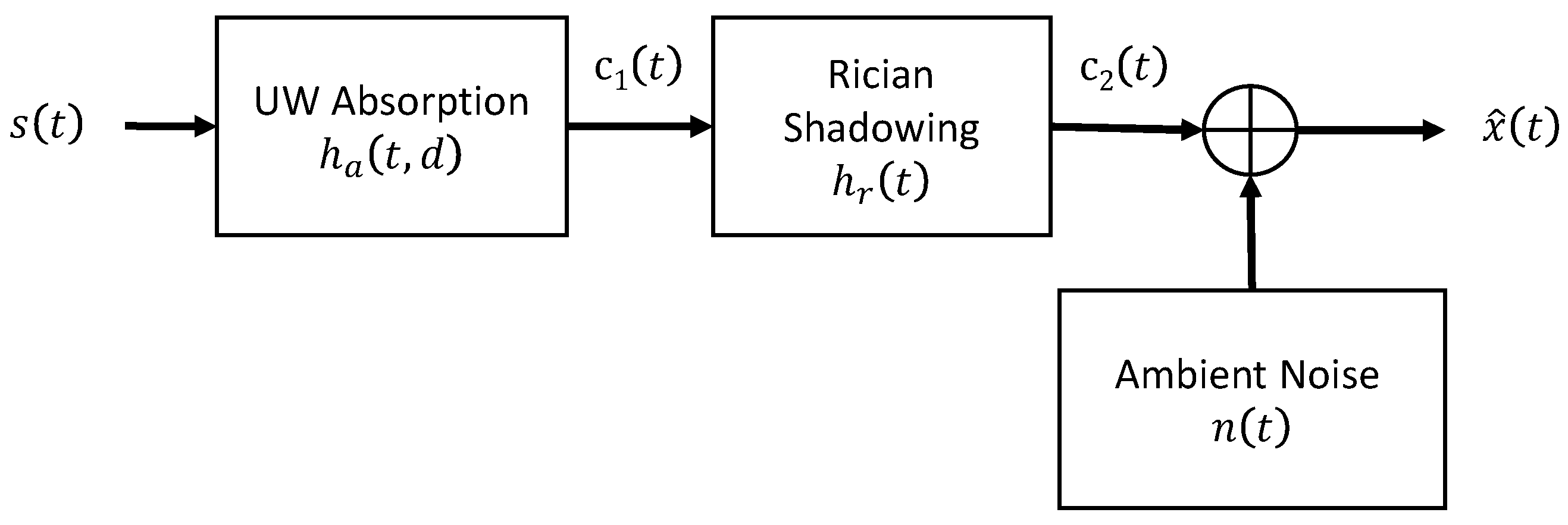
Considering to be the CPM modulated time domain digital signal from Equation (1), Figure 5 shows it passing through the channel blocks. This allows for controlling the SNR, modifying channel taps and the acoustic absorption pathloss parameters from Thorp’s formula [47]. The typical delay spread for a shallow underwater acoustic channel is between to and can be as long as [48]
4.1. Deterministic Response
In an underwater medium the energy of an acoustic signal gets attenuated both as a function of distance as well as frequency, and the pathloss is a combination of geometric spreading as well as absorption. Mathematically, if the variation in time is the path frequency domain transmission loss expression in the positive direction will be:
where a scaling constant is denoted by . The channel’s deterministic transfer function [49,50] is:
where and are a scaling constant and transmitter-receiver distance, respectively, while denotes a complex propagation constant, in :
where and are absorption and phase constants, respectively. In UWA channels the absorption is a function of frequency as acoustic pressure is reduced due to energy losses in heat. According to the Thorp formula [47], the absorption coefficient in computed in as:
Figure 6a shows, for multiple distances, the absorption pathloss transfer function. Similarly, phase constant in is:
where represents sound velocity [51] in , calculated as:
where and are temperature, salinity, and depth, respectively. Equation (14) is called Medwin’s equation [51]. The realistic channel values are considered with temperature between 0 to 35 °C while salinity is from 0 to 45 PPT and the supported depth is up to 1000 m. The signal in Figure 5 can be expressed as:
where represents the IFFT of the channel transfer function convolved with the transmitted signal .
4.2. Random Channel
Various fading models exist for RF channels and there is a general agreement between scientists and researchers over their usage. However, the domain of fading models for UWA channels is still open and lacks consensus. Experimental studies conducted suggest that a Rician fading model accurately represents the fading observed by acoustic signals in a UWA channel [52]. Researchers studied sea trial data, with Rician shadowed distribution having the closet fit [53,54]. The parameters selected in this work are and [54]. The value of spreading factor can also be assumed [55]. The signal from Figure 5 can be represented as:
where and are noise and Rician fading [56] impulse response modelled using Rician channel object in MATLAB R2019b by MathWorks, respectively. Figure 6b shows the sample of channel path gains and delay profile.
4.3. Ambient Noise
In a realistic UWA channel, the noise is not white and depends upon various acoustic frequencies. For our simulations, we use an ambient noise model that is a combination of thermal, shipping, wave, and turbulence noise [57]. The power spectral density (PSD) of the total noise is:
The noise is location specific and can be modeled as color noise, and its amplitude is high at both the lower and upper end of the spectrum while minimum around 60 kHz [58].
5. Simulation Results
The performance of the proposed system was evaluated using simulations where a CPM-OFDM transceiver is communicating over a UWA channel. The simulation parameters used are shown in Table 1.
We selected the values of the modulation index by varying the numerator from 1 to 15. We chose the values of the denominator by varying it from 2 to 16 such that remains rational. This gave us a total of 23 values of . Any other values outside this set do not give any better performance, and we found this set to be sufficient to assess the performance of the intended system. Moreover, selecting higher values of and would result in higher number of points in the constellation, increasing the decoder complexity. The error performance of a typical CPM-OFDM system for these 23 values of is shown in Figure 7.
Based upon the BER values, the curves have been divided into two categories: A and B. As is evident from Figure 7, Category A represents those curves that show good BER performance, whereas Category B represents those curves that show poor BER performance. The best BER is achieved when the value of is either or . The BER performance for these two values of is not identical but because they are very close, they appear to be overlapping each other.
In addition to these two values, there are more curves in Figure 7 that appear to be overlapping each other. Therefore, we have also shown the BER performance using two tables—Table 2 and Table 3. The difference between these two tables is the way they have been sorted. Table 2 is sorted on and , and Table 3 has been sorted on the BER values when SNR is 20 dB.
It is evident that the best BER is achieved when is which has been highlighted with a yellow color. The performance of is very similar to the case when and is highlighted with an orange color. In both these cases, the number of points in the constellation will be , i.e., 32. If a smaller number of points are desired in the constellation to decrease the decoder complexity, then values with a smaller could be selected, such as that gives 16 points in the signal constellation at a slightly inferior BER. Another choice could be that would give only 10 points in the signal constellation at the cost of BER. From the two tables, it is observed that in Category A, there is only one value of that has an even value of and it is . Although it gives the minimum number of points in the signal constellation, its BER is much inferior when compared to the best case of or .
The BER performance of the proposed scheme with varying transmitter-receiver distances is shown in Figure 8. Although performance degradation as the distance increases is obvious, CPM-OFDM still gives acceptable BER up to 1.5 km. Figure 9 illustrates the BER performance as a function of channel bandwidth. The lowest BER is noted for a channel bandwidth of 10 kHz. It is also noted that, as would be expected, the BER degrades as the channel bandwidth decreases. However, the BER performance for channel bandwidths of 5 kHz and 2.5 kHz are very similar with the BER offered by 2.5 kHz being slightly better than that offered by a bandwidth of 5 kHz.
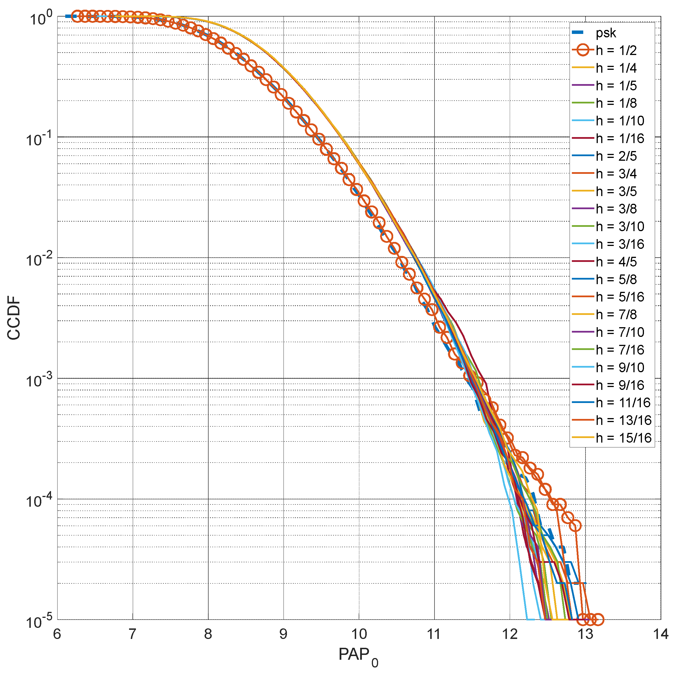
We also evaluated the PAPR performance of CPM-OFDM for all the 23 values of . The complementary cumulative distribution function (CCDF) for each value of is plotted in Figure 10. For comparison, the CCDF of a typical PSK-OFDM scheme is also plotted. The best PAPR is observed when which is almost identical to that of PSK-OFDM. The PAPR of other values of is marginally inferior to PSK-OFDM and .
6. Conclusions
Through computer simulations, it has been shown that CPM-OFDM is an attractive candidate for underwater acoustic communication. This scheme offers an excellent error performance without employing any equalization technique. The best error performance is achieved when the CPM modulation index is chosen as either 7/16 or 9/16. Moreover, acceptable error performance is observed up to a transmitter-receiver distance of 500 m. The PAPR performance of CPM-OFDM has also been evaluated and shown to be similar to those offered by other traditional OFDM schemes. Hence, a PAPR reduction technique is mandatory when employing CPM-OFDM for underwater acoustic communication. In this work, we evaluated the performance of binary CPM-OFDM and without any PAPR reduction technique. The performance of M-ary CPM-OFDM with PAPR reduction technique remains to be studied.
Author Contributions
M.M. and I.A.T. conceived the idea and the block diagram of the system. M.M. and I.A.T. implemented the model in MATLAB, ran the simulations, and wrote the manuscript. P.O. conceived and designed the UWA channel model used and contributed to the discussion section. I.A.T. and P.O. reviewed the final version of the manuscript. All authors have read and agreed to the published version of the manuscript.
Funding
The publication of this article has been funded by the Universidad de Málaga, Campus de Excelencia Internacional Andalucía Tech.
Institutional Review Board Statement
Not applicable.
Informed Consent Statement
Not applicable.
Data Availability Statement
Not applicable.
Acknowledgments
Authors express their gratitude to the Escuela Técnica Superior de Ingeniería de Telecomunicación, and the Instituto de Ingeniería Oceánica, Universidad de Málaga, Málaga, Spain. We would also like to thank College of Computer and Information Systems, Umm Al-Qura University, Makkah, Saudi Arabia.
Conflicts of Interest
The authors declare no conflict of interest.
References
- Xu, X.; Zhaohui, W.; Shengli, Z.; Wan, L. Parameterizing Both Path Amplitude and Delay Variations of Underwater Acoustic Channels Forblock Decoding of Orthogonal Frequency Division Multiplexing. J. Acoust. Soc. Am. 2012, 131, 4672–4679. [Google Scholar] [CrossRef] [Green Version]
- Stojanovic, M.; Preisig, J. Underwater Acoustic Communication Channels: Propagation Models and Statistical Characterization. IEEE Commun. Mag. 2009, 47, 84–89. [Google Scholar] [CrossRef]
- Li, B.; Zhou, S.; Stojanovic, M.; Freitag, L. Pilot-Tone Based Zp-Ofdm Demodulation for an Underwater Acoustic Channel; IEEE: New York, NY, USA, 2006. [Google Scholar]
- Mohsin, M.; Tasadduq, I.A.; Otero, P.; Poncela, J. Flexible Ofdm Transceiver for Underwater Acoustic Channel: Modeling, Implementation and Parameter Tuning. Wirel. Pers. Commun. 2021, 116, 1423–1441. [Google Scholar]
- Gang, Q.; Babar, Z.; Ma, L.; Liu, S.; Wu, J. Mimo-Ofdm Underwater Acoustic Communication Systems—A Review. Phys. Commun. 2017, 23, 56–64. [Google Scholar]
- Sean, M.; Anstett, R.; Anicette, N.; Zhou, S. A Broadband Underwater Acoustic Modem Implementation Using Coherent Ofdm. In Proceedings of the The National Conference On Undergraduate Research (NCUR), Dominican University of California, San Rafael, CA, USA, 12–14 April 2007. [Google Scholar]
- Stojanovic, M. Low Complexity Ofdm Detector for Underwater Acoustic Channels. Oceans 2006, 2006, 1–6. [Google Scholar]
- Aulin, T.; Sundberg, C.-E. Bounds on the Performance of Binary Cpfsk Type of Signaling with Input Data Symbol Pulse Shaping. In Proceedings of the NTC’78 National Telecommunications Conference, Birmingham, UK, 3–6 December 1978; Volume 1. [Google Scholar]
- Aulin, T.; Sundberg, C. Continuous Phase Modulation-Part I: Full Response Signaling. IEEE Trans. Commun. 1981, 29, 196–209. [Google Scholar] [CrossRef]
- Aulin, T.; Rydbeck, N.; Sundberg, C.-E. Continuous Phase Modulation-Part II: Partial Response Signaling. IEEE Trans. Commun. 1981, 29, 210–225. [Google Scholar] [CrossRef]
- Sun, Y. Optimal Parameter Design of Continuous Phase Modulation for Future Gnss Signals. IEEE Access 2021, 9, 58487–58502. [Google Scholar] [CrossRef]
- Peng, B.; Rossi, P.S.; Dong, H.; Kansanen, K. Time-Domain Oversampled Ofdm Communication in Doubly-Selective Underwater Acoustic Channels. IEEE Commun. Lett. 2015, 19, 1081–1084. [Google Scholar] [CrossRef]
- Proakis, J.G.; Salehi, M. Digital Communications; McGraw-Hill: New York, NY, USA, 2008. [Google Scholar]
- Kassan, K.; Farès, H.; Glattli, D.C.; Louët, Y. Performance Vs. Spectral Properties for Single-Sideband Continuous Phase Modulation. IEEE Trans. Commun. 2021, 69, 4402–4416. [Google Scholar] [CrossRef]
- Güntürkün, U.; Vandendorpe, L. Low-Complexity Lmmse–Sic Turbo Receiver for Continuous Phase Modulation, Based on a Multiaccess–Multipath Analogy. IEEE Trans. Commun. 2020, 68, 7672–7686. [Google Scholar] [CrossRef]
- Xu, Z.; Wang, Q. Autocorrelation Function of Full-Response Cpm Signals and Its Application to Synchronization. IEEE Access 2019, 7, 133781–133786. [Google Scholar] [CrossRef]
- Tasadduq, I.A.; Rao, R.K. Ofdm-Cpm Signals. Electron. Lett. 2002, 38, 80–81. [Google Scholar] [CrossRef]
- Imran, A.T.; Raveendra, K.R. Detection of Ofdm-Cpm Signals over Multipath Channels. In Proceedings of the 2002 IEEE International Conference on Communications, Conference Proceedings, ICC 2002, New York, NY, USA, 28 April–2 May 2002. [Google Scholar]
- Tasadduq, I.A.; Rao, R.K. Ofdm-Cpm Signals for Wireless Communications. Can. J. Electr. Comput. Eng. 2003, 28, 19–25. [Google Scholar] [CrossRef]
- Tasadduq, I.A.; Rao, R.K. Performance of Optimum and Suboptimum Ofdm-Cpm Receivers over Multipath Fading Channels. Wirel. Commun. Mob. Comput 2005, 5, 365–374. [Google Scholar] [CrossRef]
- Tasadduq, I.A.; Rao, R.K. Viterbi Decoding of Ofdm-Cpm Signals. Arab. J. Sci. Eng. 2003, 28, 71–80. [Google Scholar]
- Tasadduq, I.A.; Rao, R.K. Ofdm-Cpm Signals for Indoor Wireless Communications. In Proceedings of the 14th International Conference on Wireless Communications, Calgary, AB, Canada, 8–10 July 2002. [Google Scholar]
- Wylie, M.; Green, G. On the Performance of Serially Concatenated Cpm-Ofdma Schemes for Aeronautical Telemetry; Air Force Flight Test Center: Edwards, CA, USA, 2011.
- Hisojo, M.A.; Lebrun, J.; Deneire, L. Zero-Forcing Approach for L2-Orthogonal St-Codes with Cpm-Ofdm Schemes and Frequency Selective Rayleigh Fading Channels. In Proceedings of the 2014 IEEE Military Communications Conference, Baltimore, MD, USA, 6–8 October 2014. [Google Scholar]
- Morioka, K.; Kanada, N.; Futatsumori, S.; Kohmura, A.; Yonemoto, N.; Sumiya, Y.; Asano, D. An Implementation of Cpfsk-Ofdm Systems by Using Software Defined Radio. In Proceedings of the 2014 IEEE Annual Conference on Wireless and Microwave Technology (WAMICON), Tampa, FL, USA, 6 June 204.
- Tasadduq, I.A.; Rao, R.K. Papr Reduction of Ofdm Signals Using Multiamplitude Cpm. Electron. Lett. 2002, 38, 915–917. [Google Scholar] [CrossRef]
- Thompson, S.C.; Ahmed, A.U.; Proakis, J.G.; Zeidler, J.R.; Geile, M.J. Constant Envelope Ofdm. IEEE Trans. Commun. 2008, 56, 1300–1312. [Google Scholar] [CrossRef]
- Thompson, S.C.; Ahmed, A.U.; Proakis, J.G.; Zeidler, J.R. Constant Envelope Ofdm Phase Modulation: Spectral Containment, Signal Space Properties and Performance. In Proceedings of the IEEE MILCOM 2004 Military Communications Conference, Monterey, CA, USA, 31 October–3 November 2004. [Google Scholar]
- Tasadduq, I.A. Novel Ofdm-Cpm Signals for Wireless Communications: Properties, Receivers and Performance. Ph.D. Thesis, University of Western Ontario, London, ON, Canada, 2002. [Google Scholar]
- Hassan, E.S.; Zhu, X.; El Khamy, S.E.; Dessouky, M.I.; El Dolil, S.A.; El Samie, F.E.A. Performance Evaluation of Ofdm and Single-Carrier Systems Using Frequency Domain Equalization and Phase Modulation. Int. J. Commun. Syst. 2011, 24, 1–13. [Google Scholar] [CrossRef]
- Hassan, E.S.; Zhu, X.; El-Khamy, S.E.; Dessouky, M.I.; El-Dolil, S.A.; El-Samie, F.E.A. Chaotic Interleaving Scheme for Single-and Multi-Carrier Modulation Techniques Implementing Continuous Phase Modulation. J. Frankl. Inst. 2013, 350, 770–789. [Google Scholar] [CrossRef]
- Kiviranta, M.; Mammela, M.; Cabric, D.; Sobel, D.A.; Brodersen, R.W. Constant Envelope Multicarrier Modulation: Performance Evaluation Awgn and Fading Channels. In Proceedings of the MILCOM 2005 IEEE Military Communications Conference, Atlantic City, NJ, USA, 17–20 October 2005. [Google Scholar]
- Tan, J.; Stuber, L. Constant Envelope Multi-Carrier Modulation. In Proceedings of the 2002 Military Communications Conference (MILCOM), Anaheim, CA, USA, 7–10 October 2002. [Google Scholar]
- Anderson, J.B.; Aulin, T. Digital Phase Modulation; Plenum: New York, NY, USA, 1986. [Google Scholar]
- Viterbi, A. Error Bounds for Convolutional Codes and an Asymptotically Optimum Decoding Algorithm. IEEE Trans. Inf. Theory 1967, 13, 260–269. [Google Scholar] [CrossRef] [Green Version]
- Omura, J. On the Viterbi Decoding Algorithm. IEEE Trans. Inf. Theory 1969, 15, 177–179. [Google Scholar] [CrossRef]
- Kobayashi, H. Correlative Level Coding and Maximum-Likelihood Decoding. IEEE Trans. Inf. Theory 1971, 17, 586–594. [Google Scholar] [CrossRef]
- Forney, G.D. The Viterbi Algorithm. Proc. IEEE 1973, 61, 268–278. [Google Scholar] [CrossRef]
- Hayes, J.F. The Viterbi Algorithm Applied to Digital Data Transmission. IEEE Commun. Mag. 2002, 40, 26–32. [Google Scholar] [CrossRef]
- Hayes, J. The Viterbi Algorithm Applied to Digital Data Transmission. Commun. Soc. 1975, 13, 15–20. [Google Scholar] [CrossRef]
- Sklar, B. Digital Communications: Fundamentals and Applications, 2nd ed.; Prentice-Hall: Englewood Cliffs, NJ, USA, 2001. [Google Scholar]
- Haykin, S. Communication Systems; John Wiley & Sons: Hoboken, NJ, USA, 2008. [Google Scholar]
- Liu, C.; Zakharov, Y.V.; Chen, T. Doubly Selective Underwater Acoustic Channel Model for a Moving Transmitter/Receiver. IEEE Trans. Veh. Technol. 2012, 61, 938–950. [Google Scholar]
- Bocus, M.J.; Agrafiotis, D.; Doufexi, A. Underwater Acoustic Video Transmission Using Mimo-Fbmc. In Proceedings of the 2018 OCEANS-MTS/IEEE Kobe Techno-Oceans (OTO), Kobe, Japan, 28–31 May 2018. [Google Scholar]
- Wang, X.; Wang, J.; He, L.; Song, J. Doubly Selective Underwater Acoustic Channel Estimation with Basis Expansion Model. In Proceedings of the 2017 IEEE International Conference on Communications (ICC), Paris, France, 21–25 May 2017. [Google Scholar]
- Stojanovic, M. Underwater Acoustic Communications: Design Considerations on the Physical Layer. In Proceedings of the 2008 Fifth Annual Conference on Wireless on Demand Network Systems and Services, Garmisch-Partenkirchen, Germany, 23–25 January 2008. [Google Scholar]
- Urick, R.J. Sound Propagation in the Sea; Peninsula Publishing: Westport, CT, USA, 1982. [Google Scholar]
- Wan, L. Underwater Acoustic Ofdm: Algorithm Design, Dsp Implementation, and Field Performance. Ph.D. Thesis, University of Connecticut, Mansfield, CT, USA, 2014. [Google Scholar]
- Philip, M.M.; Ingard, K.U. Theoretical Acoustics; Princeton University Press: Princeton, NJ, USA, 1986. [Google Scholar]
- Roth, P.O. Fundamentos de Propagación de Ondas; Universidad de Malaga, Manual: Malaga, Spain, 2015. [Google Scholar]
- Medwin, H. Speed of Sound in Water: A Simple Equation for Realistic Parameters. J. Acoust. Soc. Am. 1975, 58, 1318–1319. [Google Scholar] [CrossRef]
- Kulhandjian, H.; Melodia, T. Modeling Underwater Acoustic Channels in Short-Range Shallow Water Environments. In Proceedings of the International Conference on Underwater Networks & Systems, Rome, Italy, 12–14 November 2014. [Google Scholar]
- Radosevic, A.; Proakis, J.G.; Stojanovic, M. Statistical Characterization and Capacity of Shallow Water Acoustic Channels. In Proceedings of the OCEANS 2009—EUROPE, Bremen, Germany, 11–14 May 2009. [Google Scholar]
- Ruiz-Vega, F.; Clemente, M.C.; Paris, J.F.; Otero, P. Ricean Shadowed Statistical Characterization of Shallow Water Acoustic Channels for Wireless Communications. In IEEE Conf. Underwater Communications: Channel Modelling & Validation, UComms; IEEE: Sestri Levante, Italy, 2012. [Google Scholar]
- Melodia, T.; Kulhandjian, H.; Kuo, L.; Demirors, E. Mobile Ad Hoc Networking: Cutting Edge Directions. In Advances in Underwater Acoustic Networking; John Wiley & Sons: Hoboken, NJ, USA, 2013. [Google Scholar]
- Jeruchim, M.; Balaban, P.; Shanmugan, K.S. Simulation of Communication Systems, 2nd ed.; Kluwer Academic/Plenum: New York, NY, USA, 2000. [Google Scholar]
- Stojanovic, M. On the Relationship between Capacity and Distance in an Underwater Acoustic Communication Channel. ACM SIGMOBILE Mob. Comput. Commun. Rev. 2007, 11, 34–43. [Google Scholar] [CrossRef]
- Hebbar, R.P.; Poddar, P.G. Generalized Frequency Division Multiplexing–Based Acoustic Communication for Underwater Systems. Int. J. Commun. Syst. 2020, 33, e4292. [Google Scholar] [CrossRef]
Figure 1.
Proposed CPM-OFDM transceiver for underwater acoustic channel.
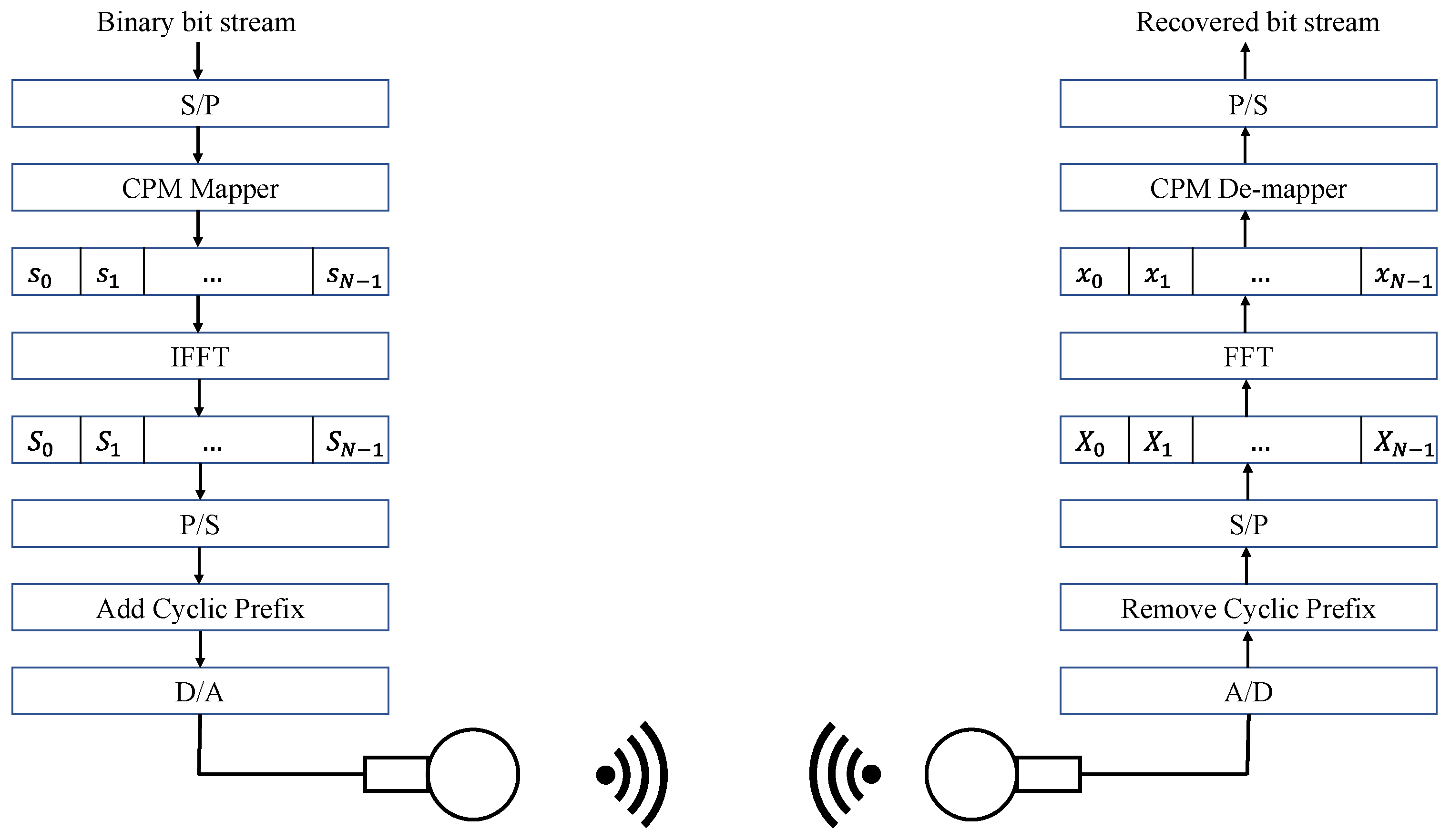
Figure 2.
Trellis diagram for h = 1/2.

Figure 3.
Constellation diagram for (a) h = 2/5 (b) h = 1/4.
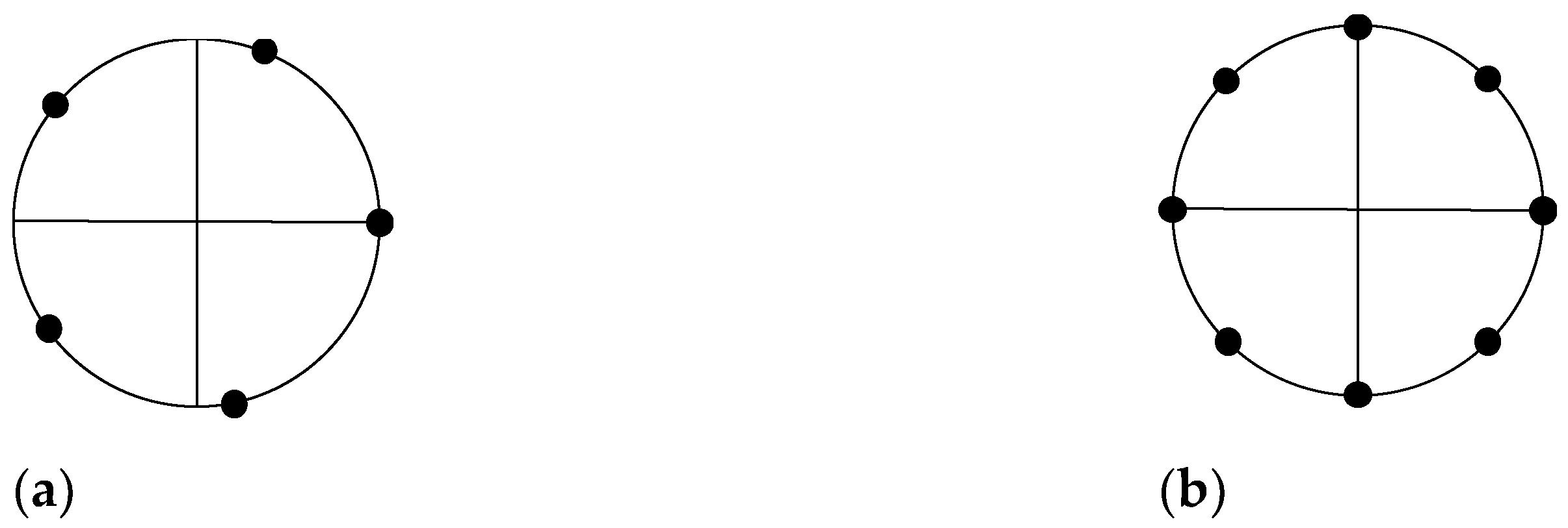
Figure 4.
All the possible paths through the trellis for h = 1/2. Solid lines indicate bit 1, broken lines indicate bit 0, and bold lines indicate a typical bit sequence of 1011. The complex numbers beside the figure are the possible CPM mapper output.
Figure 4.
All the possible paths through the trellis for h = 1/2. Solid lines indicate bit 1, broken lines indicate bit 0, and bold lines indicate a typical bit sequence of 1011. The complex numbers beside the figure are the possible CPM mapper output.

Figure 5.
Shallow underwater acoustic channel model.

Figure 6.
Shallow acoustic channel characteristics: (a) frequency dependent absorption; (b) channel impulse response.
Figure 6.
Shallow acoustic channel characteristics: (a) frequency dependent absorption; (b) channel impulse response.
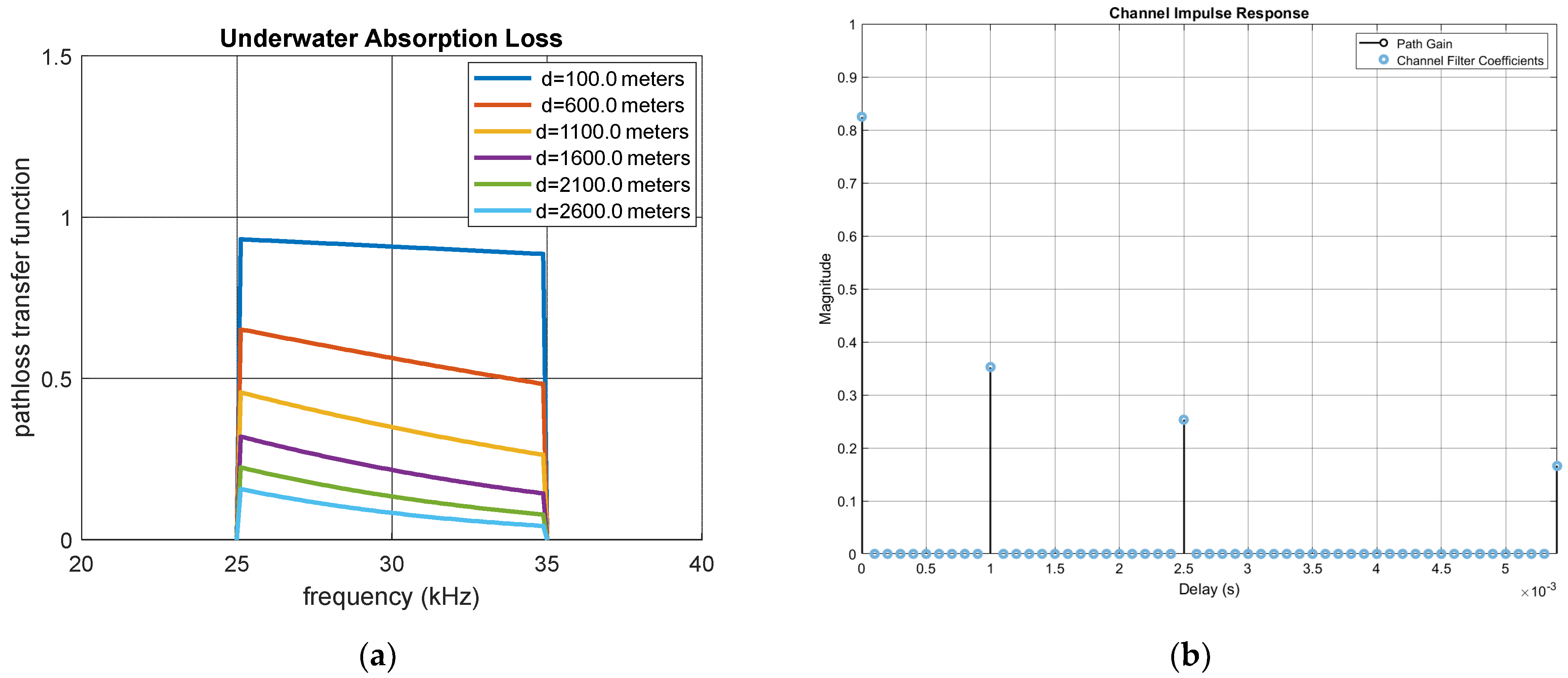
Figure 7.
Error performance of CPM-OFDM for 23 rational values of modulation index h with N = 512 and transmitter-receiver distance 500 m.
Figure 7.
Error performance of CPM-OFDM for 23 rational values of modulation index h with N = 512 and transmitter-receiver distance 500 m.
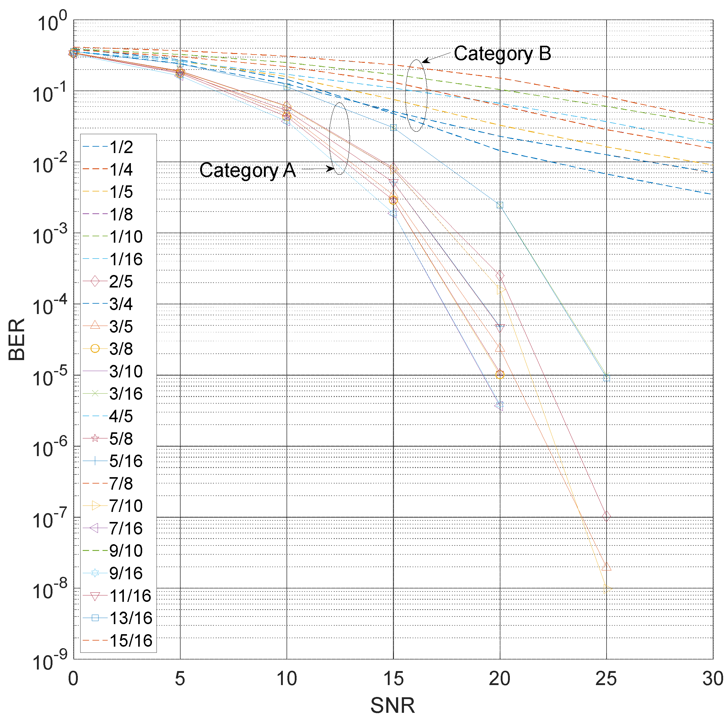
Figure 8.
BER performance of CPM-OFDM as a function of transmitter-receiver distances with , .
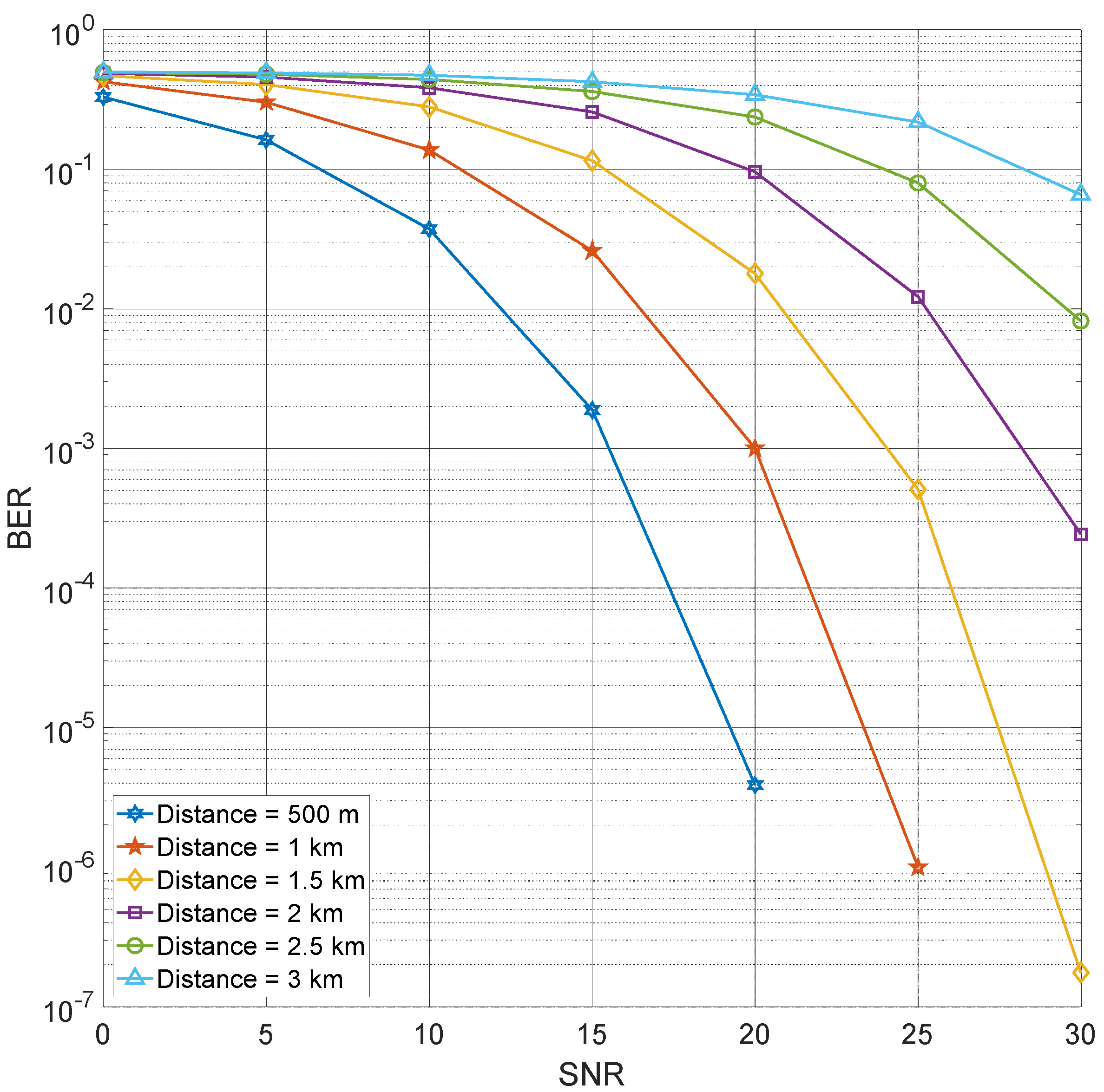
Figure 9.
BER performance of CPM-OFDM as a function of channel bandwidth with , .
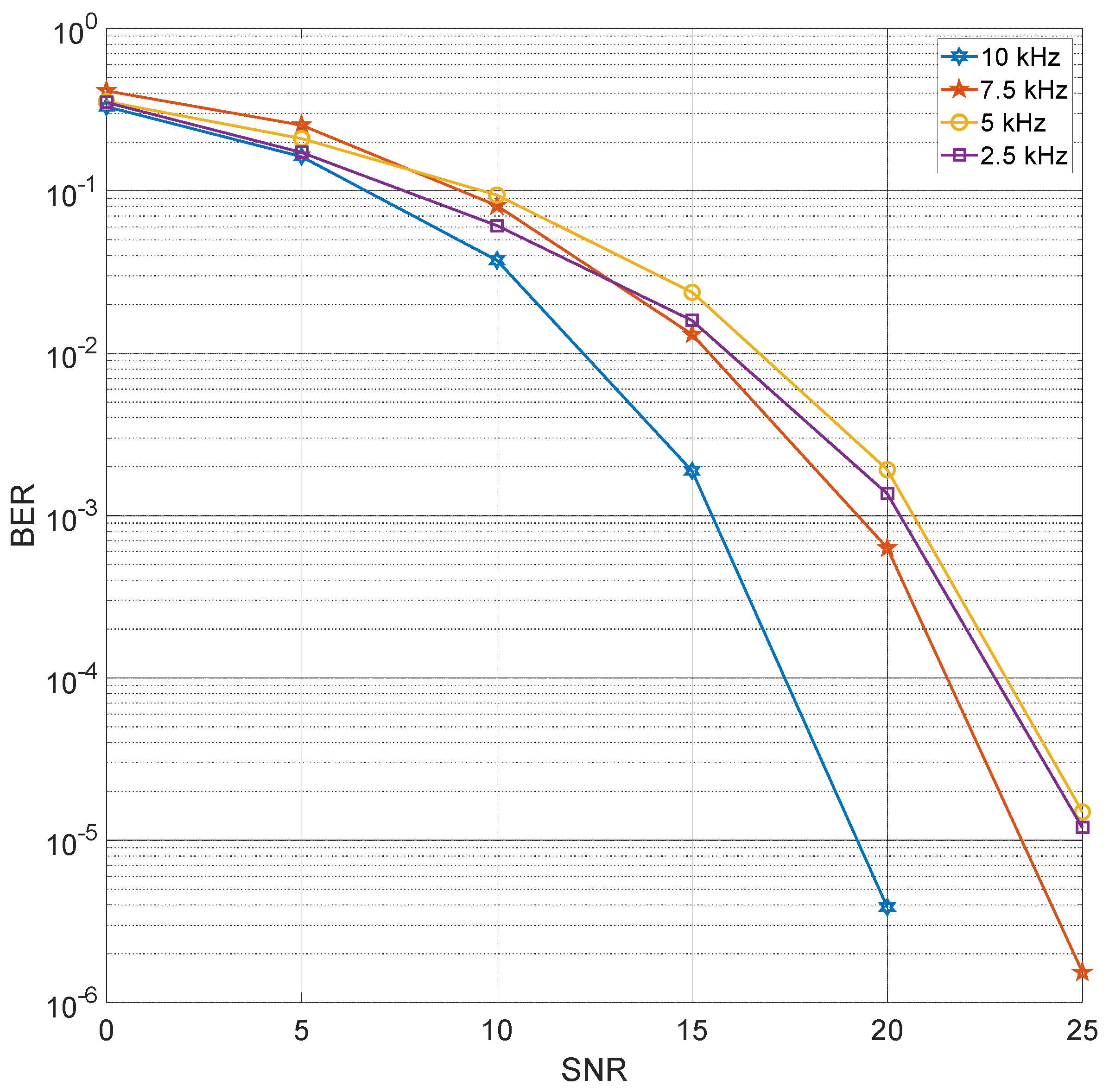
Figure 10.
PAPR performance of CPM-OFDM as a function of 23 values of with and transmitter-receiver distance 500 m.
Figure 10.
PAPR performance of CPM-OFDM as a function of 23 values of with and transmitter-receiver distance 500 m.


Table 1.
Simulation parameters.
| Parameters | Values |
|---|---|
| Number of Subcarriers | 512 |
| CP Length | 128 (typically, 1/4th the no. of subcarriers) |
| Modulation Index | 23 rational values |
| Bandwidth | 10 kHz |
| Average Path Gains | dB |
| Path Delays | ms |
| Sampling Frequency | 10,000 samples per second |
| OFDM Symbol Duration | 51.2 ms |
| No. of OFDM Symbols Transmitted | 160,000 |
| No. of Simulation Runs | 20 |
| Tx-Rx Distance | 500 m |
| Transmitter Depth | 50 m |
| Receiver Depth | 50 m |
| Doppler Frequency | 10 Hz |
| Atmospheric pressure | Pa |
| Salinity | 35 parts/1000 |
| Density | 103 kg/m3 |
| Water temperature | 25 °C |
Table 2.
BER values for various modulation indices and SNRs (sorted on values of p and q).
| SNR (dB) | ||||||||
|---|---|---|---|---|---|---|---|---|
| 0 | 5 | 10 | 15 | 20 | 25 | 30 | ||
| 1 | 2 | 0.389864 | 0.274086 | 0.145444 | 0.04784 | 0.01437 | 0.006743 | 0.003461 |
| 1 | 4 | 0.358647 | 0.241738 | 0.124955 | 0.051068 | 0.022901 | 0.012591 | 0.007052 |
| 1 | 5 | 0.360902 | 0.261278 | 0.158968 | 0.075665 | 0.032758 | 0.016251 | 0.009047 |
| 1 | 8 | 0.377929 | 0.303389 | 0.219292 | 0.132342 | 0.06248 | 0.028433 | 0.015397 |
| 1 | 10 | 0.388773 | 0.325632 | 0.250118 | 0.169976 | 0.10423 | 0.060461 | 0.033599 |
| 1 | 16 | 0.412185 | 0.367027 | 0.307857 | 0.232441 | 0.151332 | 0.082683 | 0.039188 |
| 2 | 5 | 0.343899 | 0.189986 | 0.06111 | 0.008237 | 0.00025 | 0 | |
| 3 | 4 | 0.358597 | 0.241657 | 0.124931 | 0.051127 | 0.022885 | 0.012581 | 0.007057 |
| 3 | 5 | 0.343854 | 0.186318 | 0.047827 | 0.003423 | 0 | ||
| 3 | 8 | 0.337594 | 0.175321 | 0.043152 | 0.002893 | 0 | 0 | |
| 3 | 10 | 0.341311 | 0.188547 | 0.059988 | 0.007768 | 0.00016 | 0 | |
| 3 | 16 | 0.357686 | 0.239549 | 0.113669 | 0.030198 | 0.002457 | 0 | |
| 4 | 5 | 0.360941 | 0.261225 | 0.170811 | 0.109233 | 0.06671 | 0.0368 | 0.018393 |
| 5 | 8 | 0.337572 | 0.175237 | 0.043122 | 0.002893 | 0 | 0 | |
| 5 | 16 | 0.337189 | 0.180792 | 0.052542 | 0.005163 | 0 | 0 | |
| 7 | 8 | 0.37788 | 0.303382 | 0.219266 | 0.132345 | 0.06243 | 0.028404 | 0.015389 |
| 7 | 10 | 0.341236 | 0.188574 | 0.059911 | 0.00778 | 0.000159 | 0 | |
| 7 | 16 | 0.329276 | 0.162725 | 0.037263 | 0.001883 | 0 | 0 | |
| 9 | 10 | 0.388748 | 0.325557 | 0.250039 | 0.169949 | 0.104257 | 0.060448 | 0.033613 |
| 9 | 16 | 0.329302 | 0.16274 | 0.037281 | 0.001882 | 0 | 0 | |
| 11 | 16 | 0.337094 | 0.180739 | 0.052517 | 0.005183 | 0 | 0 | |
| 13 | 16 | 0.357658 | 0.239519 | 0.113663 | 0.030164 | 0.002452 | 0 | |
| 15 | 16 | 0.412149 | 0.367034 | 0.30793 | 0.232537 | 0.151276 | 0.082633 | 0.039155 |
Table 3.
BER values for various modulation indices and SNRs (sorted on values of BER at SNR = 20 dB).
Table 3.
BER values for various modulation indices and SNRs (sorted on values of BER at SNR = 20 dB).
| SNR (dB) | |||||||||
|---|---|---|---|---|---|---|---|---|---|
| 0 | 5 | 10 | 15 | 20 | 25 | 30 | |||
| Category A | 7 | 16 | 0.329276 | 0.162725 | 0.037263 | 0.001883 | 0 | 0 | |
| 9 | 16 | 0.329302 | 0.16274 | 0.037281 | 0.001882 | 0 | 0 | ||
| 3 | 8 | 0.337594 | 0.175321 | 0.043152 | 0.002893 | 0 | 0 | ||
| 5 | 8 | 0.337572 | 0.175237 | 0.043122 | 0.002893 | 0 | 0 | ||
| 3 | 5 | 0.343854 | 0.186318 | 0.047827 | 0.003423 | 0 | |||
| 11 | 16 | 0.337094 | 0.180739 | 0.052517 | 0.005183 | 0 | 0 | ||
| 5 | 16 | 0.337189 | 0.180792 | 0.052542 | 0.005163 | 0 | 0 | ||
| 7 | 10 | 0.341236 | 0.188574 | 0.059911 | 0.00778 | 0.000159 | 0 | ||
| 3 | 10 | 0.341311 | 0.188547 | 0.059988 | 0.007768 | 0.00016 | 0 | ||
| 2 | 5 | 0.343899 | 0.189986 | 0.06111 | 0.008237 | 0.00025 | 0 | ||
| 13 | 16 | 0.357658 | 0.239519 | 0.113663 | 0.030164 | 0.002452 | 0 | ||
| 3 | 16 | 0.357686 | 0.239549 | 0.113669 | 0.030198 | 0.002457 | 0 | ||
| Category B | 1 | 2 | 0.389864 | 0.274086 | 0.145444 | 0.04784 | 0.01437 | 0.006743 | 0.003461 |
| 3 | 4 | 0.358597 | 0.241657 | 0.124931 | 0.051127 | 0.022885 | 0.012581 | 0.007057 | |
| 1 | 4 | 0.358647 | 0.241738 | 0.124955 | 0.051068 | 0.022901 | 0.012591 | 0.007052 | |
| 1 | 5 | 0.360902 | 0.261278 | 0.158968 | 0.075665 | 0.032758 | 0.016251 | 0.009047 | |
| 7 | 8 | 0.37788 | 0.303382 | 0.219266 | 0.132345 | 0.06243 | 0.028404 | 0.015389 | |
| 1 | 8 | 0.377929 | 0.303389 | 0.219292 | 0.132342 | 0.06248 | 0.028433 | 0.015397 | |
| 4 | 5 | 0.360941 | 0.261225 | 0.170811 | 0.109233 | 0.06671 | 0.0368 | 0.018393 | |
| 1 | 10 | 0.388773 | 0.325632 | 0.250118 | 0.169976 | 0.10423 | 0.060461 | 0.033599 | |
| 9 | 10 | 0.388748 | 0.325557 | 0.250039 | 0.169949 | 0.104257 | 0.060448 | 0.033613 | |
| 15 | 16 | 0.412149 | 0.367034 | 0.30793 | 0.232537 | 0.151276 | 0.082633 | 0.039155 | |
| 1 | 16 | 0.412185 | 0.367027 | 0.307857 | 0.232441 | 0.151332 | 0.082683 | 0.039188 | |
Publisher’s Note: MDPI stays neutral with regard to jurisdictional claims in published maps and institutional affiliations. |
© 2021 by the authors. Licensee MDPI, Basel, Switzerland. This article is an open access article distributed under the terms and conditions of the Creative Commons Attribution (CC BY) license (https://creativecommons.org/licenses/by/4.0/).
Share and Cite
MDPI and ACS Style
Tasadduq, I.A.; Murad, M.; Otero, P. CPM-OFDM Performance over Underwater Acoustic Channels. J. Mar. Sci. Eng. 2021, 9, 1104. https://doi.org/10.3390/jmse9101104
AMA Style
Tasadduq IA, Murad M, Otero P. CPM-OFDM Performance over Underwater Acoustic Channels. Journal of Marine Science and Engineering. 2021; 9(10):1104. https://doi.org/10.3390/jmse9101104
Chicago/Turabian StyleTasadduq, Imran A., Mohsin Murad, and Pablo Otero. 2021. "CPM-OFDM Performance over Underwater Acoustic Channels" Journal of Marine Science and Engineering 9, no. 10: 1104. https://doi.org/10.3390/jmse9101104
Note that from the first issue of 2016, this journal uses article numbers instead of page numbers. See further details here.