Detection and Analysis of the Causes of Intensive Harmful Algal Bloom in Kamchatka Based on Satellite Data

Abstract

In this paper, the causes of the anomalous harmful algal bloom which occurred in the fall of 2020 in Kamchatka have been detected and analyzed using a long-term time series of heterogeneous satellite and simulated data with respect to the sea surface height (HYCOM) and temperature (NOAA OISST), chlorophyll-a concentration (MODIS Ocean Color SMI), slick parameters (SENTINEL-1A/B), and suspended matter characteristics (SENTINEL-2A/B, C2RCC algorithm). It has been found that the harmful algal bloom was preceded by temperature anomalies (reaching 6 °C, exceeding the climatic norm by more than three standard deviation intervals) and intensive ocean level variability followed by the generation of vortices, mixing water masses and providing nutrients to the upper photic layer. The harmful algal bloom itself was manifested in an increase in the concentration of chlorophyll-a, its average monthly value for October 2020 (bloom peak) approached 15 mg/m³, exceeding the climatic norm almost four-fold for the region of interest (Avacha Gulf). The zones of accumulation of a large amount of biogenic surfactant films registered in radar satellite imagery correlate well with the local regions of the highest chlorophyll-a concentration. The harmful bloom was influenced by river runoff, which intensively brought mineral and biogenic suspensions into the marine environment (the concentration of total suspended matter within the plume of the Nalycheva River reached 10 mg/m³ and more in 2020), expanding food resources for microalgae.

1. Introduction

Harmful algal blooms are dangerous natural processes which are difficult to be predicted or prevented. It is necessary to study these processes [1]. Such a task can be effectively solved using satellite remote sensing data [2] through the application of specialized methods of their processing [3,4,5].

Satellite monitoring methods have a wide range of capabilities to study marine water areas which include wide coverage; efficiency; capability to work in any hard-to-reach areas of seas and oceans; obtaining data of various spatial and temporal resolution in different electromagnetic wave spectral regions; a wide range of registered parameters of water environment; and high reliability of obtained data [6]. The efficiency of these methods is largely increased when combining them with sea truth and modeling results [7,8]. The abovementioned features provide for the high efficiency of marine water area remote sensing when solving various thematic tasks related with coastal water area pollution detection, including to study and monitor microalgae blooming [9,10].

Up-to-date scientific publications on the topic of this paper shows that the problem of satellite data application for monitoring and studying harmful algal blooms (HAB) can have different formulations. On the one hand, specialized methods and algorithms for satellite (mostly, optical multispectral) data processing are being developed and applied that allow for the creation of information products aimed directly at detecting and determining algae type and describing conditions of HABs. The examples of such efforts include a red tide index study [11,12], use of machine learning algorithms for automatic distinction of various types of environmental conditions and HAB detection in satellite optical imagery [3], use of a special algorithm for algae detection for various waters [4], studying the alternative floating algae index (AFAI) [5], et al.

On the other hand, comprehensive studies applying a large amount of heterogeneous data are carried out that are aimed at the understanding of natural processes occurring during HAB preparation and development. Algal blooms are driven by various factors including physical and chemical ones. Physical factors include horizontal inhomogeneity and stratification of water, water illumination and temperature, wind, currents, and tides. Chemical factors include a high level of available mineral and organic nutrients coming from coastal runoffs, and excreta of hydrobionts from both atmospheric precipitation and from bottom sediments during vertical water movements [1,13,14,15].

Taking this into account, it is possible to study HAB conditions and development features using a time series of well-proven standard information products of satellite oceanography, such as chlorophyll-a concentration in the near-surface layer of the marine environment and sea surface temperature. For example, in [7,8,16], to monitor HAB development and to reveal the causes of its occurrence, various combinations of standard information products are used, formed on the basis of data from satellite spectroradiometers MODIS, SeaWiFS, and MERIS (sea surface temperature, chlorophyll-a etc.), as well as HYCOM and NCEP products describing the ocean level, current, and near-surface wind characteristics. A very important significant water environment parameter registered by satellite methods for HAB study is chlorophyll-a. The effort [17] is focused on a detailed analysis of chlorophyll-a concentration variability for HAB monitoring purposes. This effort, “Detection and analysis of the causes of intensive harmful algal bloom in Kamchatka based on satellite data”, carries on the abovementioned comprehensive research. Here we develop an original technique for analyzing large arrays of heterogeneous data from satellite oceanology to study a single large-scale HAB case.

This study was conducted in coastal waters east of Kamchatka. Kamchatka is a pen-insula in the northeastern part of Eurasia, surrounded from the west by the Sea of Okhotsk, and from the east by the Bering Sea and the Pacific Ocean.

On the southeastern coast of the peninsula there is the Avacha Gulf, where this study was carried out (see Figure 1, red polygon). The area of the Avacha Gulf is ~2400 km². The depths of the Avacha Gulf vary. After the elevations of 150–200 m, there is a sharp slope, turning into the valleys of the Pacific Ocean. The climate of Avacha Bay, due to its exposure, is extremely unstable; the gulf is open to winds and sea waves. The Kamchatka Current passes along the eastern coast of the Kamchatka Peninsula, which includes Avacha Gulf. The water temperature in winter varies from 1 °C to 3 °C, and in summer months the water warms up to an average of 15 °C [18].

From the end of September to the beginning of October 2020, an intensive harmful algal bloom (hereinafter referred to as HAB) was registered in the coastal water areas of the Kamchatka peninsula. This phenomenon caused a massive loss of aquatic organisms, health problems of people who contacted with water, produced plenty of foam on the coast, and created unnatural seawater color [9]. Most of these negative phenomena were observed in the coastal zone of the Avacha Gulf about 40 km long from the Spaseniya Bay to the Listvennichnaya Bay, including the Khalaktyrsky Beach. The map of the region of interest showing the locations of negative HAB effects is given in Figure 1.

Intense HABs are accompanied by a series of negative effects, in particular, toxins released by microalgae enter the water environment, which have a detrimental effect on hydrobionts (up to their death) and the entire ecosystem as a whole [1,13].

This effort is dedicated to the detection and analysis of causes of the intensive Kamchatka 2020 HAB according to satellite data of various types.

2. Materials and Methods

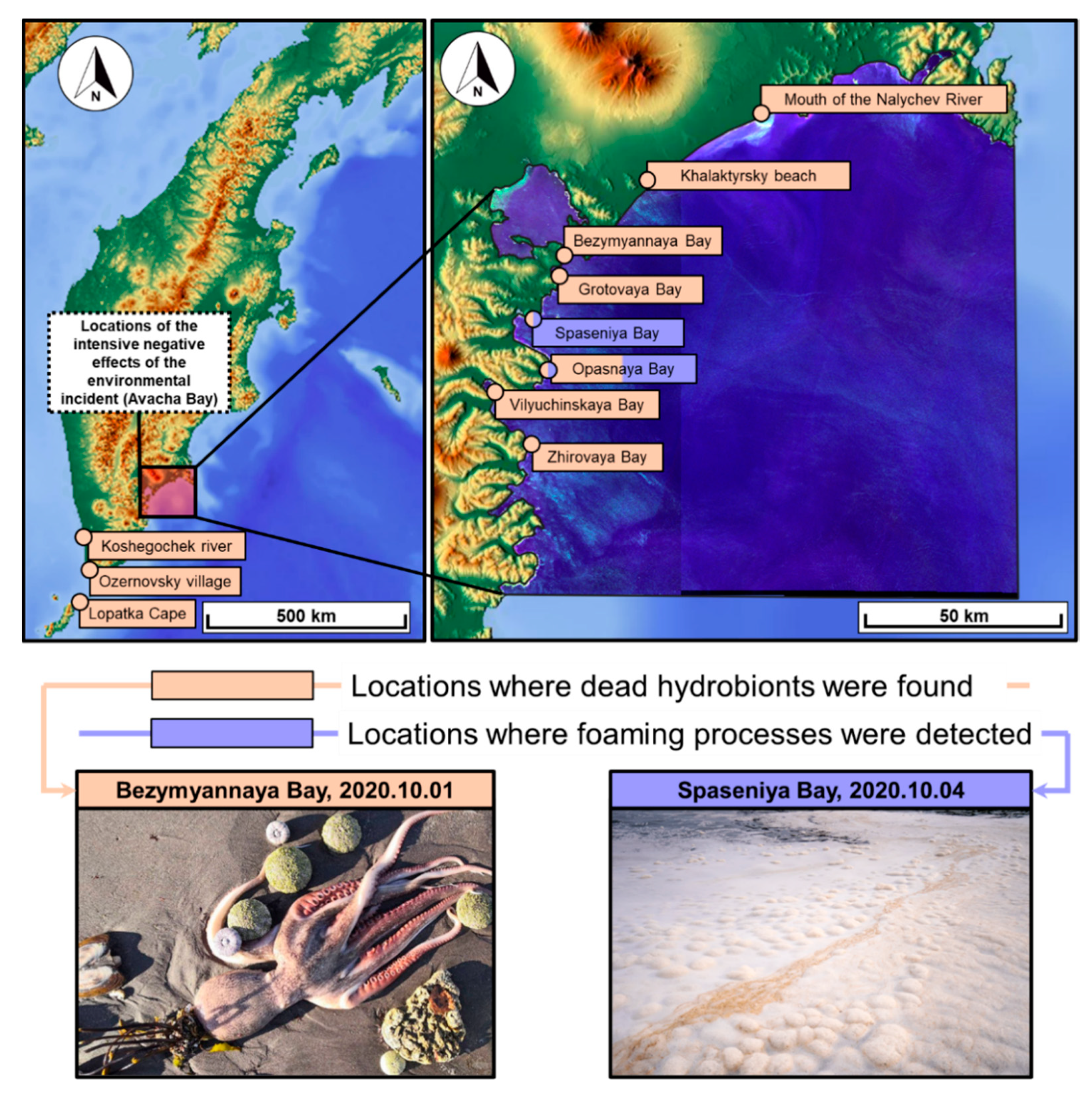
2.1. General

Our research is based on the analysis of long-term time series of inhomogeneous source satellite data on the sea surface characteristics and the estimates of variability of key factors causing and affecting the development of a HAB in the studied region. The following source satellite and simulated data were used: HYCOM sea surface height [19], and NOAA OISST sea surface temperature [20] data. LAS information product (Live Access Server): Aviso+ was applied to interpret HYCOM data [21]. Also, satellite optical multispectral and radar imagery obtained by Sentinel-2A/B [22] and Sentinel-1A/B [23] satellites, respectively, were used, as well as sea surface temperature and chlorophyll-a concentrations (MODIS Ocean Color SMI [24] and NOAA VIIRS [25]).

Satellite data processing was carried out in three directions, namely:

• Processing long-term retrospective satellite data series on the ocean level, sea surface temperature, chlorophyll-a concentration to reveal precursors and indicators of HAB development in the fall of 2020.
• Processing radar satellite imagery obtained by Sentinel-1A/B during harmful algal bloom in the fall of 2020 to detect and assess the properties of slicks with their further analysis to reveal the signs of algal blooming in the region of interest.
• Processing Sentinel-2A/B optical multispectral satellite imagery in 2019 and 2020 for the region of the inflow of the Nalycheva River into the water area of interest to assess possible impact of the river runoff on HAB in the fall 2020.

During the research, first of all, the fact was taken into account that HABs with such strongly expressed negative consequences were recorded for the first time off the coast of Kamchatka.

Hence, we believe that the disaster under consideration was preceded by specific conditions of the water environment, which had not been observed previously in the studied water area.

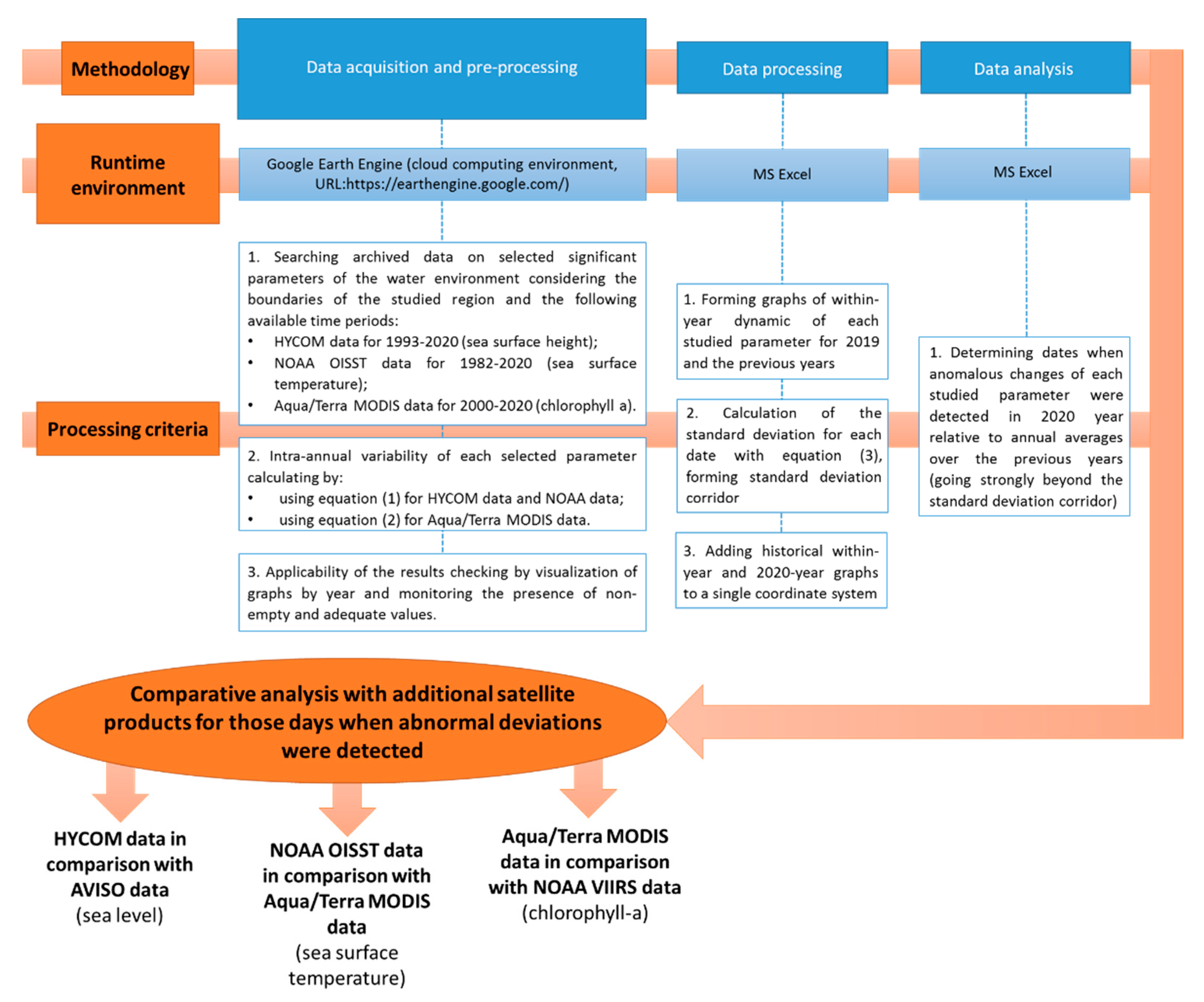
2.2. A Method for the Processing Long-Term Retrospective Series of Satellite Data on the Ocean Level, Sea Surface Temperature, Chlorophyll-a Concentration

Thus, the method for the processing long-term retrospective series of satellite data on the ocean level, sea surface temperature, and chlorophyll-a concentration was based on the comparison of the features of the dynamics of these significant parameters of the water environment in 2020 with the characteristic dynamics of the same parameters recorded in previous years in the study area of interest. The study was carried out within the Avacha Gulf water area covering certain open ocean area adjacent to the gulf (Figure 1).

As it is mentioned above, the following significant water environment parameters were used:

(a)

Sea surface height (SSH) influencing the current mode and conditions for upwelling, which in its turn is important for the formation of food resources of microalgae (data are available since 1 January 1993).

(b)

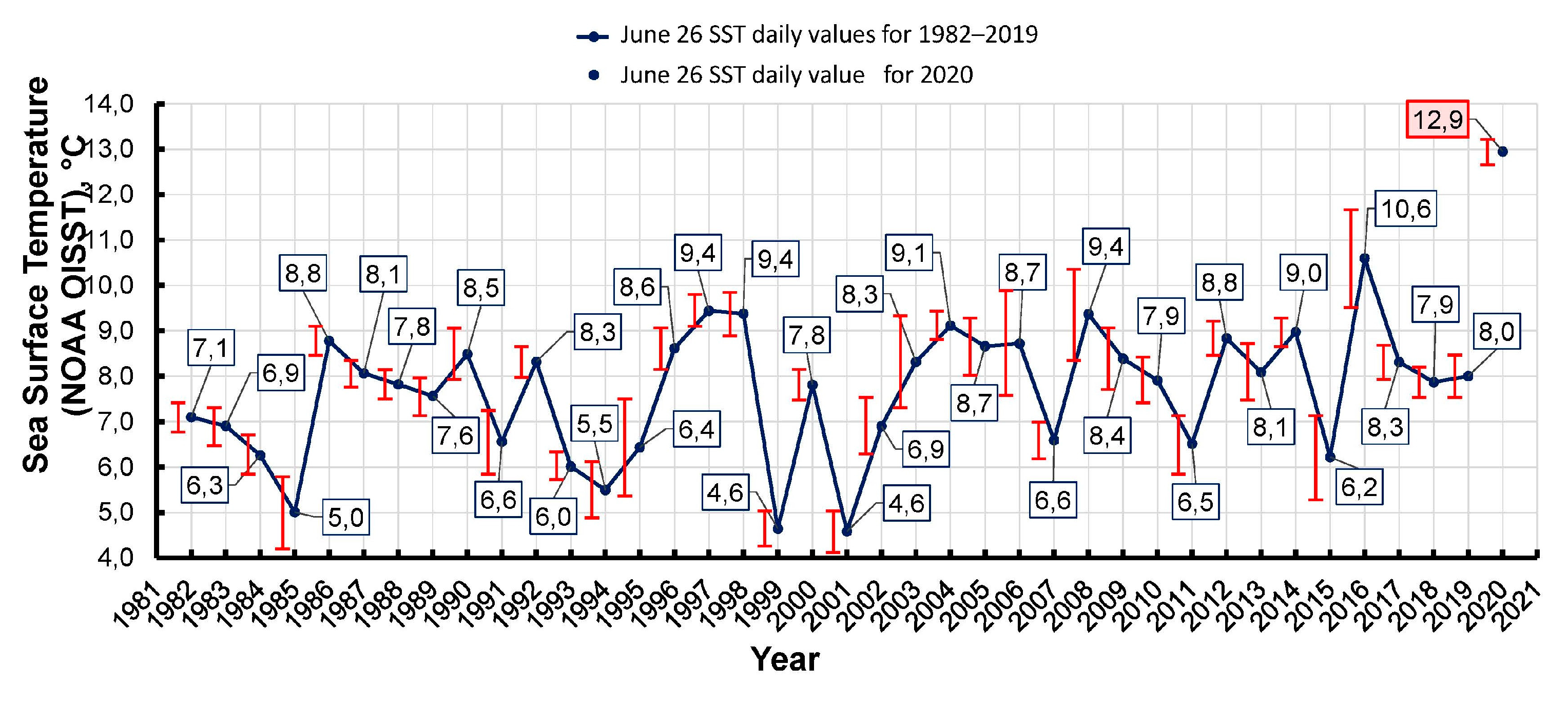
Sea surface temperature (SST) (data are available since 1 January 1982).

(c)

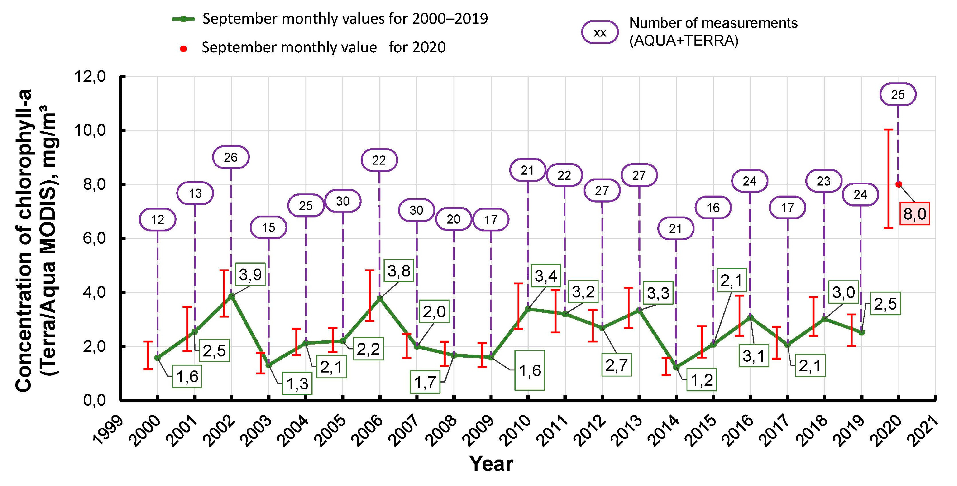
Chlorophyll-a concentration in the near surface layer of the water environment (data are available since 1 May 2000).

The method of research involved the construction and analysis of graphs showing the intra-annual variability of each studied significant parameter of the water environment within the area of interest. SST and SSH graphs were plotted with one day discreteness, which corresponded to the source temporal resolution of the information products used. The daily value of the studied parameter was averaged over the area:

$$P_{date}={{\displaystyle \sum }}_{i=1}^{n_{date}}{p}_i/n_{date},$$

(1)

where P_date is the calculated average value of the water environment parameter for the current date; $n_{date}$ is the number of measurements (nonempty pixels) within the studied area for the target date; and $p_i$ is the value of the studied parameter in the current pixel.

Chlorophyll-a concentration graphs were built with one month discreteness. The computation of $P_{month}$ monthly average values was carried out according to the principle of “cumulative average” for each element of the grid of values within the studied area:

$$P_{month}={{\displaystyle \sum }}_{i=1}^{n_{month}}{\overline{P}}_i/n_{month},$$

(2)

where P_month is the calculated average value of the water environment parameter for the current month; n_month is the number of pixels within the study area, where there was at least one measurement per month; and ${\overline{P}}_i$ is the monthly average value of the studied parameter in the current pixel.

The results of within-year dynamics of the studied water environment parameters obtained for 2019 and the previous years were generalized through the calculation of the average $\overline{P}$ value and σ standard deviation:

$${\sigma }_{date}=\sqrt{\frac{{\displaystyle \sum }{\left({\left(P_{date}\right)}_j-{ \overline{P}}_{date}\right)}^2}{N}} ,$$

(3)

where N is the number of a sample (the number of years of observations preceding the year of registration of the studied HAB—2020).

${ \overline{P}}_{date}$ graphs, together with ${\sigma }_{\mathrm{date}}$ standard deviation corridor, characterize the climatic norm well and make it possible to adequately assess the features of the temporal variability of significant parameters of the water environment recorded in 2020 during the formation of the prerequisites for the development of HABs in the ecosystem of the studied area [9]. As a result of this technique it is possible to determine dates when anomalous changes of each studied parameter of the water were detected in 2020 year relative to averages over the previous years (going strongly beyond the standard deviation corridor). Finally, comparative analysis with additional satellite products for those days when abnormal deviations were detected is performing, as shown on Figure 2.

Data acquisition and calculations using Equations (1) and (2) were carried out using the Google Earth Engine cloud infrastructure. Calculations by Equation (3) and construction of graphs were carried out in Excel. Comparative analysis with map layouts forming was carried out using the QGIS the ENVI + IDL software.

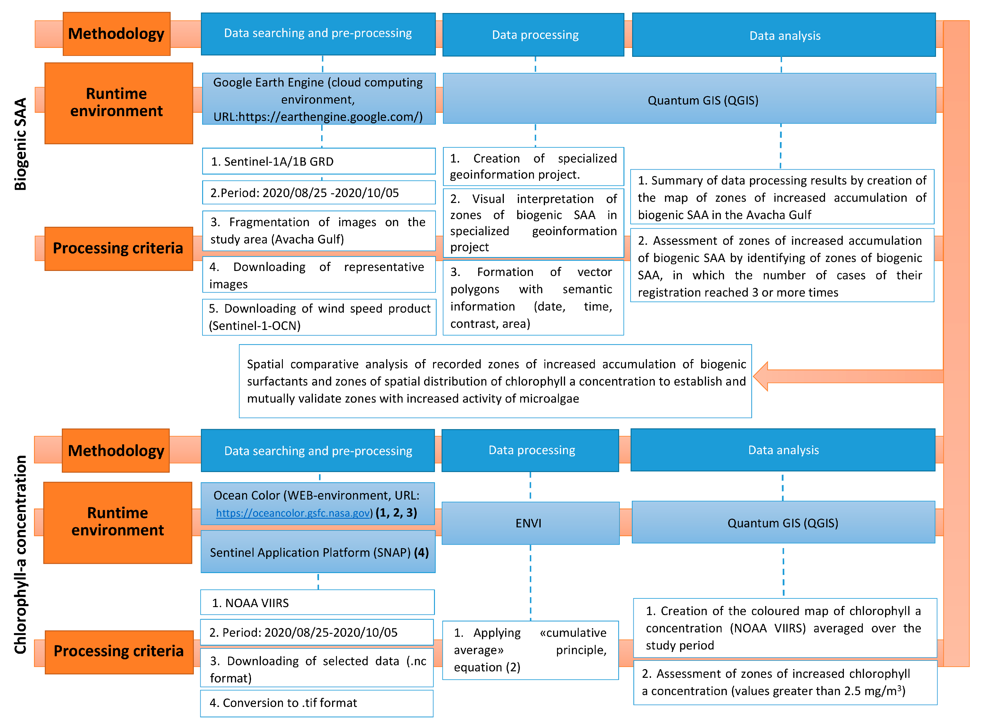
2.3. Sentinel-1A/B Radar Satellite Imagery Processing Method

In the course of the research, the processing of the Avacha Gulf Sentinel-1A/B satellite radar images was carried out (from 25 August to 5 October 2020). The processing was aimed at the detection and estimation of sea surface slick properties related with biogenic surface active agents films (later on “biogenic SAA”).

Using satellite radar images, owing to the resonant mechanism of radio wave scattering by wave-covered water surface, it is possible to monitor slick formations of both natural and anthropogenic origins [6,26]. When interpreting biogenic SAA using radar imagery, it is necessary to provide for their reliable recognition against the background of other slick-forming processes (e.g., calm belts, rain cells, internal wave surface manifestations, atmospheric gravity waves, ship spills etc.) [27].

With intensive blooming of microalgae, biogenic surfactants are formed on the sea surface causing the formation of slicks with specific interpretation features [27]. In satellite radar images, biogenic SAA usually represent a series of long (many kilometers long) often curved or spiral stripes (due to current fields). Such film formations are often observed in the coastal zones or in the upwelling zones. Biogenic surfactants exist in quite a narrow wind speed range (from 2–3 m/s to 5 m/s) [27]. Detection and assessment of the characteristics of such slick formations using satellite radar images can confirm the fact of HAB development, as well as provide detailed information on the spatial and geometric properties and dynamics of biogenic surfactant accumulations.

Flowchart for Sentinel-1A/B dataset processing is shown on Figure 3.

To increase the reliability of biogenic SAA interpretation using satellite radar imagery and to provide for the comprehensive analysis of their spatial and geometric characteristics, a specialized geoinformation project has been developed in this effort that contains source radar satellite imagery and the results of their interpretation as polygons with semantic information (date, time, contrast and area), as well as the geographic features of the studied region, meteorological data (in particular, near-surface wind characteristics), bathymetry, and etc.

Generalized results of detection of slicks related with biogenic surfactants were compared with the data on negative HAB effects (see Figure 1) and spatial chlorophyll-a concentration distributions in the Avacha Gulf obtained according to the “cumulative average” principle (see Equation (2)) for the whole period of radar imagery collection (from 25 August to 5 October 2020).

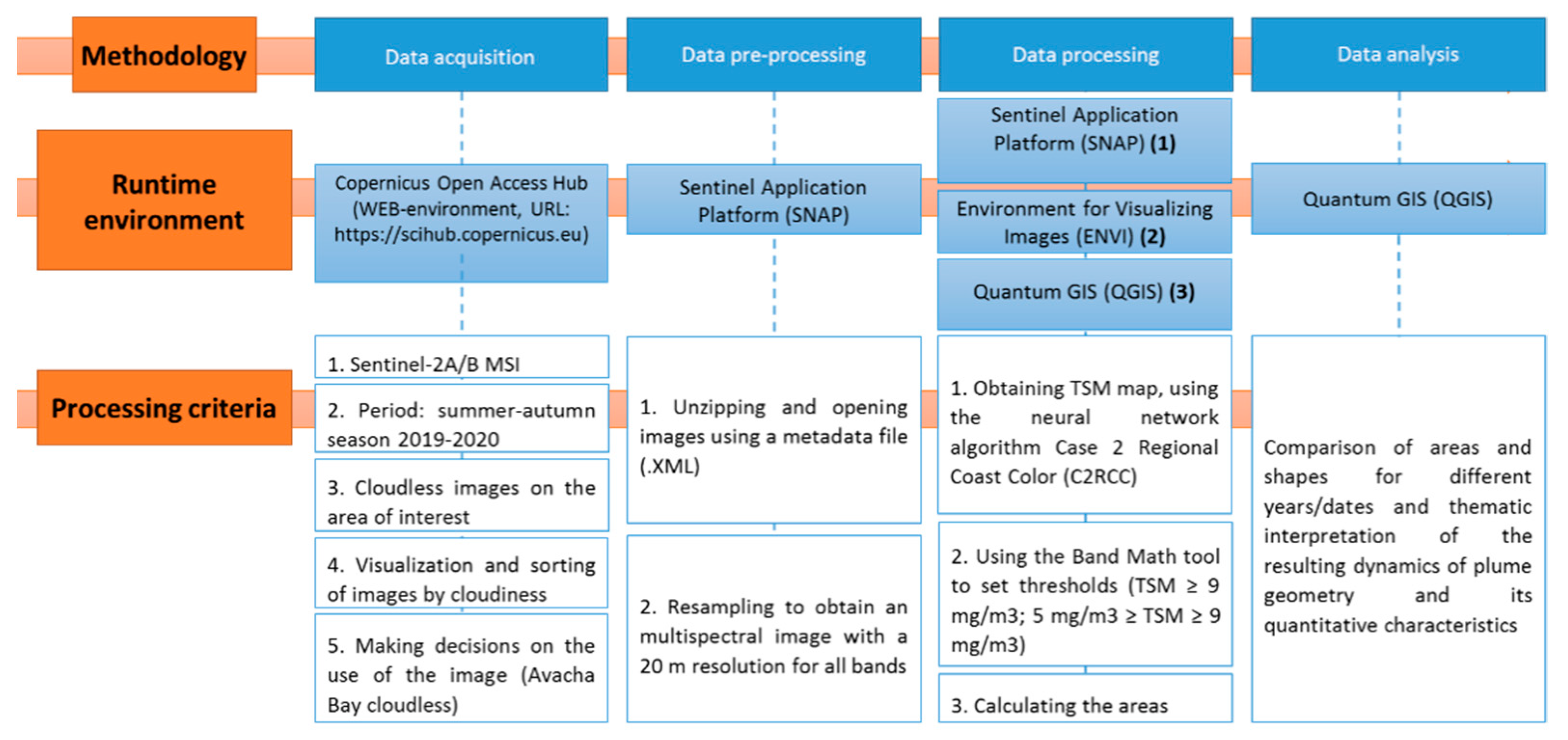
2.4. Sentinel-2A/B Multispectral Imagery Processing Method

Several rivers, including the rather large Nalycheva river, flow into the Avacha Gulf on the banks of which the most intensive negative consequences of the studied HAB were recorded. Along with the river runoff, nutrients can enter the coastal waters, contributing to the development of microalgae [1,28]. In the present study, the characteristics of the runoff of the Nalycheva River in the interests of studying the features of its influence on the process of preparation and development of intensive HAB, registered in the fall of 2020.

The processing of optical multispectral Sentinel-2A/B imagery was carried out using the automatic neural network Case 2 Regional Coast Colour (C2RCC) algorithm that allows us to assess bio-optical water environment parameters, in particular total suspended matter (TSM) in the surface layer [29,30]. Increased TSM values in marine water areas near river mouths indicate the presence of fine matter of biological and mineral origin [31], which, as a rule, contains nutrients that contribute to the development of algae [32]. TSM calculations were performed using the SNAP software (see Figure 4).

The resulting fields of TSM distributions were processed using the threshold method in order to detect a wastewater plume from the Nalycheva River. Two threshold values were used, which ensured the identification of the distribution areas of both the most saturated with suspended matter share of the river discharge (i.e., the plume “core”), and the peripheral areas of the river discharge (i.e., the “transition zone” of the plume). The following condition was used to select the “core”:

TSM ≥ 9 mg/m³

(4)

The selection of the “transition zone” was carried out with another one condition:

9 mg/m³ > TSM ≥ 5 mg/m³

(5)

Based on the results of identifying the distribution areas of the plume of the Nalycheva River, generalizing schematic maps were formed and analyzed using the geo-information environment.

3. Results and Discussion

3.1. Anomalies in Long-Term Retrospective Aeries of Satellite Data

3.1.1. Ocean Level

Figure 5 shows the graphs of the ocean level dynamics (HYCOM), obtained using the method described above for processing a retrospective data set (since 1993). The insets in Figure 5 show the sea level anomaly (SLA) and the directions of geostrophic currents obtained from the data of the LAS: Aviso + satellite altimetry information product aggregator for some dates in 2020 (when anomalous changes in the sea surface height were recorded).

Analysis of the data shown in Figure 5 revealed the following features:

• On 19 April, anomalously low SSH values were recorded relative to the annual average values (HYCOM), which can also be traced in the spatial distribution of sea level anomalies (Aviso +), presented in the inset of Figure 5. These features clearly indicate the presence of a cyclonic oceanic vortex.
• On 3 June 2020, SSH values anomalously exceeding annual average values (HYCOM) were observed, as well as such high values were observed in the spatial distribution of sea level anomalies (Aviso +), shown in the inset of Figure 5. These features clearly indicate the presence of an anticyclonic oceanic vortex in the studied water area.
• On 30 August and the 15 and 19 September 2020, anomalously high SSH values and geostrophic currents were recorded, the configuration of which also corresponded to oceanic vortexes of the anticyclonic type.

Thus, it was found that the intense HAB, which occurred in Kamchatka in the fall of 2020, was preceded by a developed SSH dynamics, characterized by the presence of predominantly positive anomalies and signs of anti-cyclonic vortexes. It should be noted that the cold Vostochno-Kamchatskoe Current passes along the southeastern coast of Kamchatka, which is accompanied by the formation of vortex structures with the subsequent generation of unsteady mesoscale phenomena, including jets and mushroom-like currents. The reason for the formation of such vortices is the influence of the bottom topography and coastline inhomogeneity on the Vostochno-Kamchatskoe Current [33]. These vortices affect the mixing of biologically productive coastal waters and open ocean waters, ensuring the flow of biogenic elements into the upper photic layer and thereby positively affecting the development of phytoplankton [34].

Examples of the positive impact of different types of vortices on the development of phytoplankton are numerous for the regions of the world’s oceans, while the mechanisms of the impact of cyclonic and anticyclonic vortices on biota can be different. In most cases, anticyclonic vortices that prevailed in the study area in 2020 are characterized by abnormally high concentrations of chlorophyll-a in the surface water layer along the vortex periphery [35].

Thus, based on the analysis of data on the ocean level dynamics in the study area, it has been established that during 2020, the situation has repeatedly evolved, contributing to the processes of preparation and development of HABs.

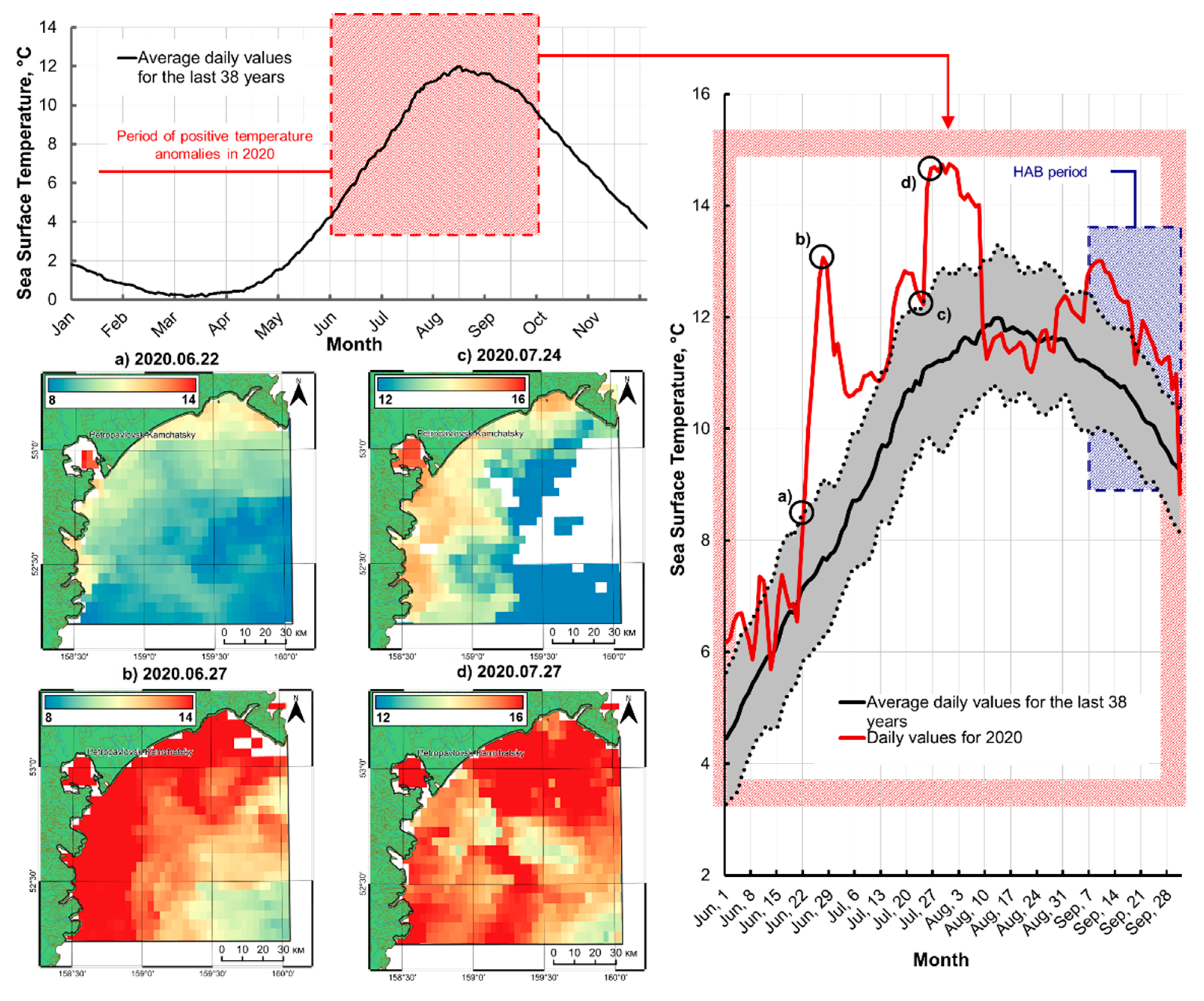
3.1.2. Sea Surface Temperature

According to the abovementioned method, the temperature of the sea surface in the studied water area was investigated using the daily information products of NOAA OISST for the period from 1981 to 2020. The obtained NOAA values of the surface temperature for 1981–2019 were averaged and compared with daily values for 2020, while detailed spatial distributions for critical dates were considered according to MODIS data (Figure 6).

From the analysis of the data shown in Figure 6, it follows that from 22 June to 12 July 2020 and from 15 July to 8 August 2020 in the study area, anomalous exceeding in sea surface temperature (reaching 6 °C) were recorded compared to average long-term values. The overshoot of sea surface temperature values recorded on 27 June 2020 exceeded 3 intervals of standard deviation. On 27 July 2020, such an overshoot exceeded 2 intervals of the standard deviation (see Figure 6). The spatial distributions of the sea surface temperature show that warm anomalies are most intensive near the coastline, in the area of registration of negative HAB manifestations. It is known (see, for example, [14]) that such positive SST anomalies have a significant effect on the biogenic mode of the upper photic layer of the seawater column and can lead to the intensive development of microalgae, causing red tides.

As follows from the analysis of Figure 6, in 2020 in the study area, warm anomalies were especially strong. In this regard, it is fair to assume that the temperature conditions in 2020 greatly contributed to the preparation and development of the HAB off the coast of Kamchatka, and the temperature factor played a key role in the development of the environmental disaster off the coast of Kamchatka.

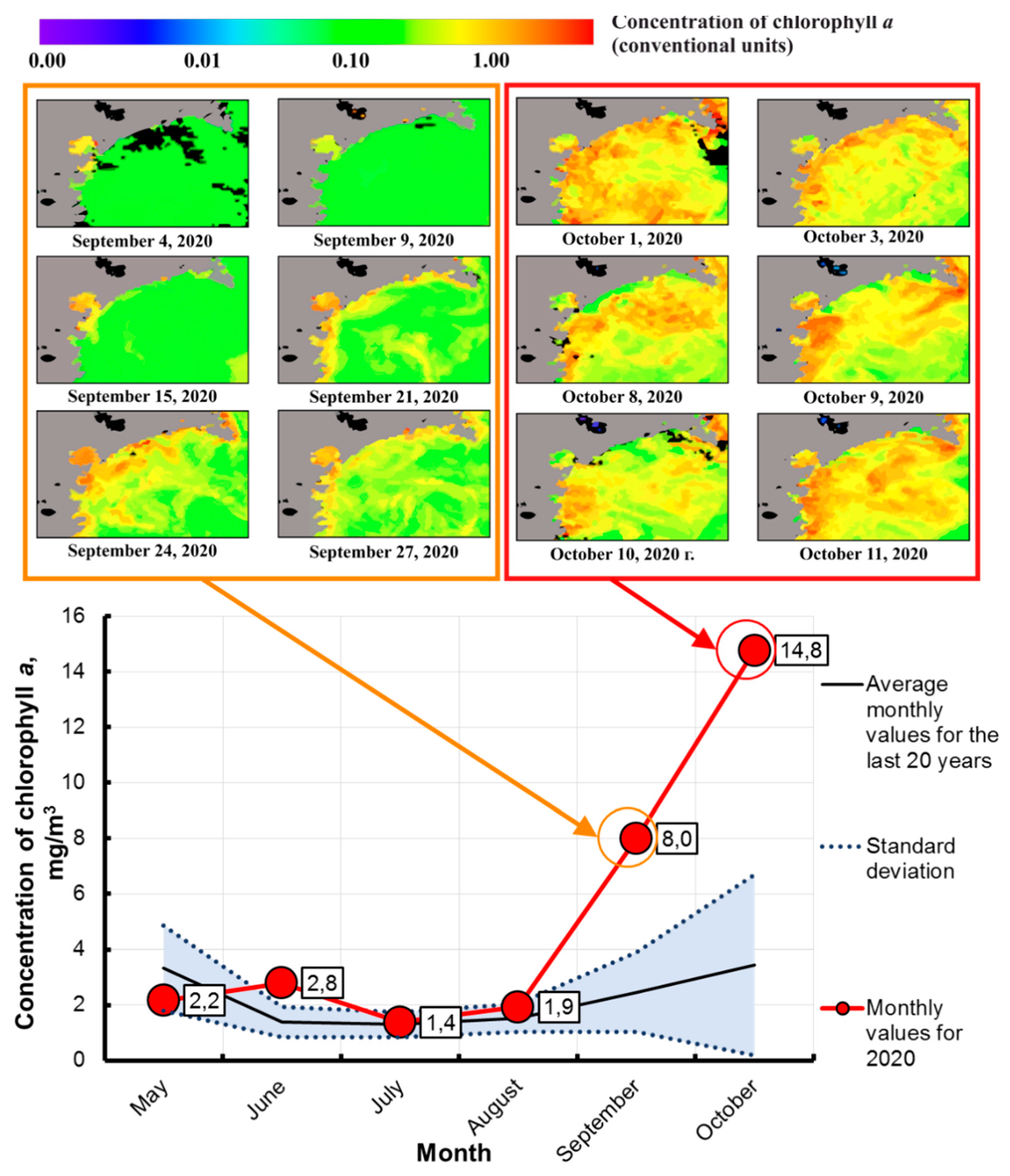
3.1.3. Chlorophyll-a Concentration

The chlorophyll-a concentration was studied using the monthly average information products MODIS Ocean Color SMI [24], obtained according to the method described above (see Figure 2) as a result of processing of a retrospective data set from 2000 to 2020 (in the periods from May to October). The resulting monthly average values for 2000–2019 were averaged and compared with the monthly average values for 2020 (see Figure 7, bottom).

Figure 7 (top) shows the spatial distributions of chlorophyll-a concentration obtained from NOAA VIIRS data [25] at the time of intense HAB development for some dates in 2020 (when the transition from the background to anomalous conditions was recorded).

An analysis of the data obtained, presented in Figure 7 (top), made it possible to reveal a sharp increase in the concentration of chlorophyll-a, which occurred in the third decade of September 2020, practically over the entire area of the Avacha Gulf, compared with the previous days. A high level of chlorophyll-a concentration in this water area was also observed in the following days, with a maximum on 1 October 2020. Compared with background values, for example, on 4 September 2020, the chlorophyll-a concentration measured on 1 October 2020 increased by approximately an order of magnitude from 0.1 to 1.0 conv. units and more (see Figure 7, top).

From the analysis of the graphs shown in Figure 7 (lower part) it follows that the values of the average monthly concentrations of chlorophyll-a in September–October 2020 significantly (more than 3.5-fold) exceeded the climatic norm; values of chlorophyll-a concentrations in the same months averaged over 2000–2019. It should be noted that satellite information products on the concentration of chlorophyll-a, calculated based on global algorithms [24,25], must be analyzed taking into account, inter alia, the regional characteristics of the studied water area and atmospheric conditions. However, the unprecedentedly high measured values of chlorophyll-a obtained in this study for October 2020 indicate significant changes in the optical properties of the near-surface layer of the marine environment caused by biological factors. The possible influence of atmospheric phenomena and the regional specificity of the optical characteristics of waters on the accuracy of the data obtained is largely compensated by the use of the accumulated averaged monthly values of chlorophyll-a concentrations for 2020 and their comparison with the monthly values of chlorophyll-a concentrations in the water area of interest, averaged over the 20-year observation period (2000–2019).

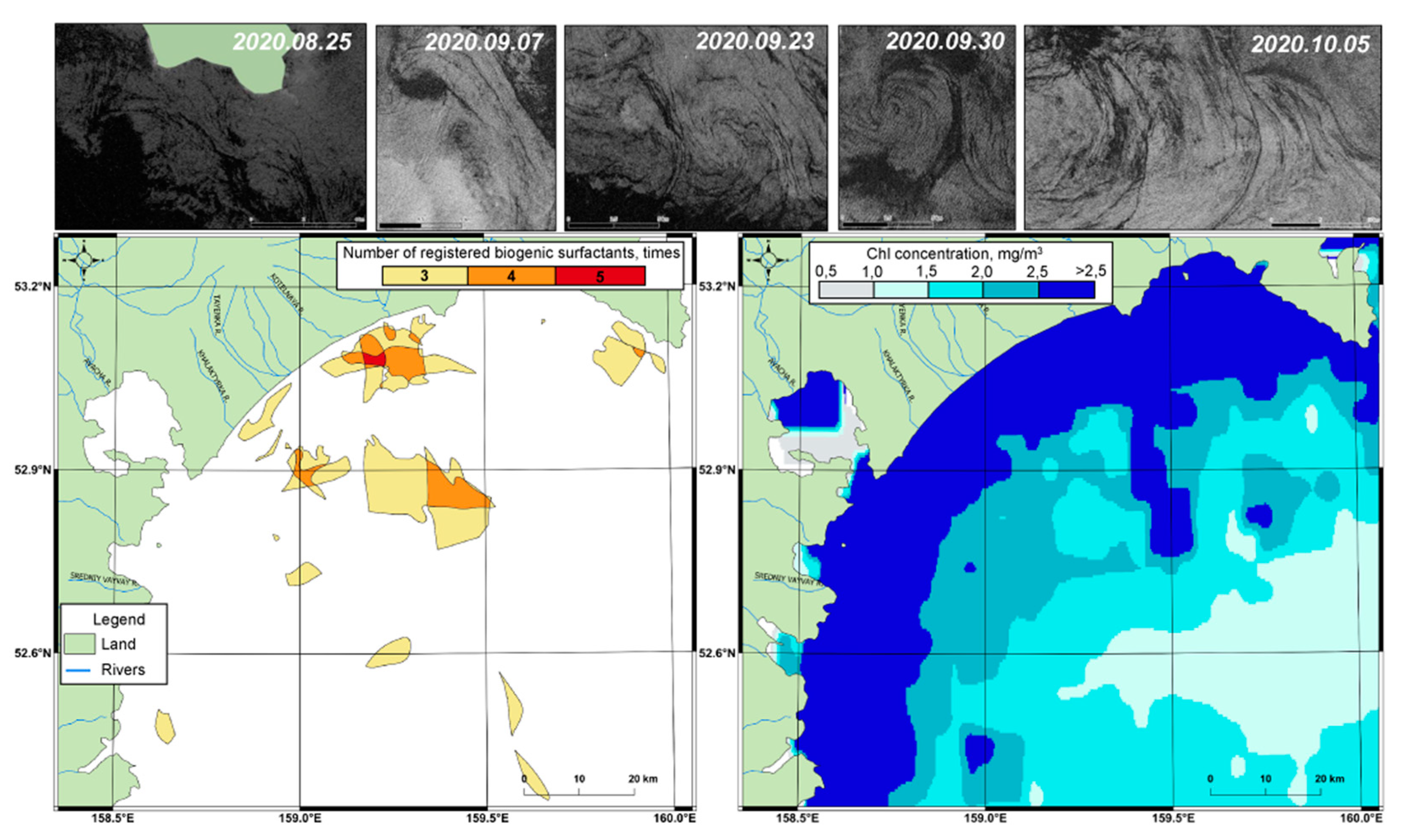
3.2. Biogenic Surfactant Films (Sentinel-1A/B)

According to the previously described method, satellite radar images obtained from the Sentinel-1A/B satellites were studied during the period from 25 August to 5 October 2020. In this case, information products of the first and second processing levels were used, including data on the characteristics of the near-surface wind (Sentinel-1-OCN).

Numerous biogenic surfactants were detected on space radar images from 25, 26, 30 August, 7, 19, 23 and 30 September, as well as 1 and 5 October 2020. Based on the results of space radar image processing, a map of zones of increased accumulation of biogenic surfactants was created, in which the number of cases of their registration reached three or more times (see Figure 8). The analysis of these data has shown that biogenic surfactants were distributed unevenly over the studied water area. In different parts of the Avacha Gulf, the number of cases of registration of biogenic surfactants ranged from 0 to 5 (over the observation period). The measured radar contrasts of the detected slicks were ~3.6 to ~5.5 dB.

Analysis of Figure 8 shows that zones of increased accumulation of biogenic SAA were most often concentrated near the coast of the Avacha Gulf. Zones of increased accumulation of biogenic surfactants, in which the number of cases of their registration was three times, were located chaotically throughout the Avacha Gulf at a distance of ~1–70 km from the coast. Zones of concentration of biogenic SAA with the number of cases of their registration 4 times were observed in the northern and northeastern parts of the Avacha Gulf at a distance of ~1–28 km from the coast. The zone most exposed to biogenic surfactants with the number of cases of their registration 5 times was located in the coastal part of the Avacha Gulf near the mouths of the Nalycheva and Kotelnaya rivers at a distance of ~4 km from the coast (coordinates of the zone are 53.1° N, 159.2° E). The total area of zones of increased accumulation of biogenic SAA, identified by the results of processing space radar images, was ~680 km².

The results of registration of zones of increased accumulation of biogenic surfactants in space radar imagery were compared with the map of the spatial distribution of chlorophyll-a concentration in the Avacha Gulf, formed according to NOAA VIIRS data (see Figure 8). As a result of the comparison, it was confirmed that high activity of microalgae was observed in the coastal strip ~25 km wide, as well as in the central part of the gulf near the point with coordinates 52.8° N and 159.5° E.

As a result of the analysis of satellite radar images, it was found that the study area during the HAB in 2020 was subjected to intense natural impacts. Attention is drawn to the large-scale nature of biogenic surfactants registered in the Avacha Gulf.

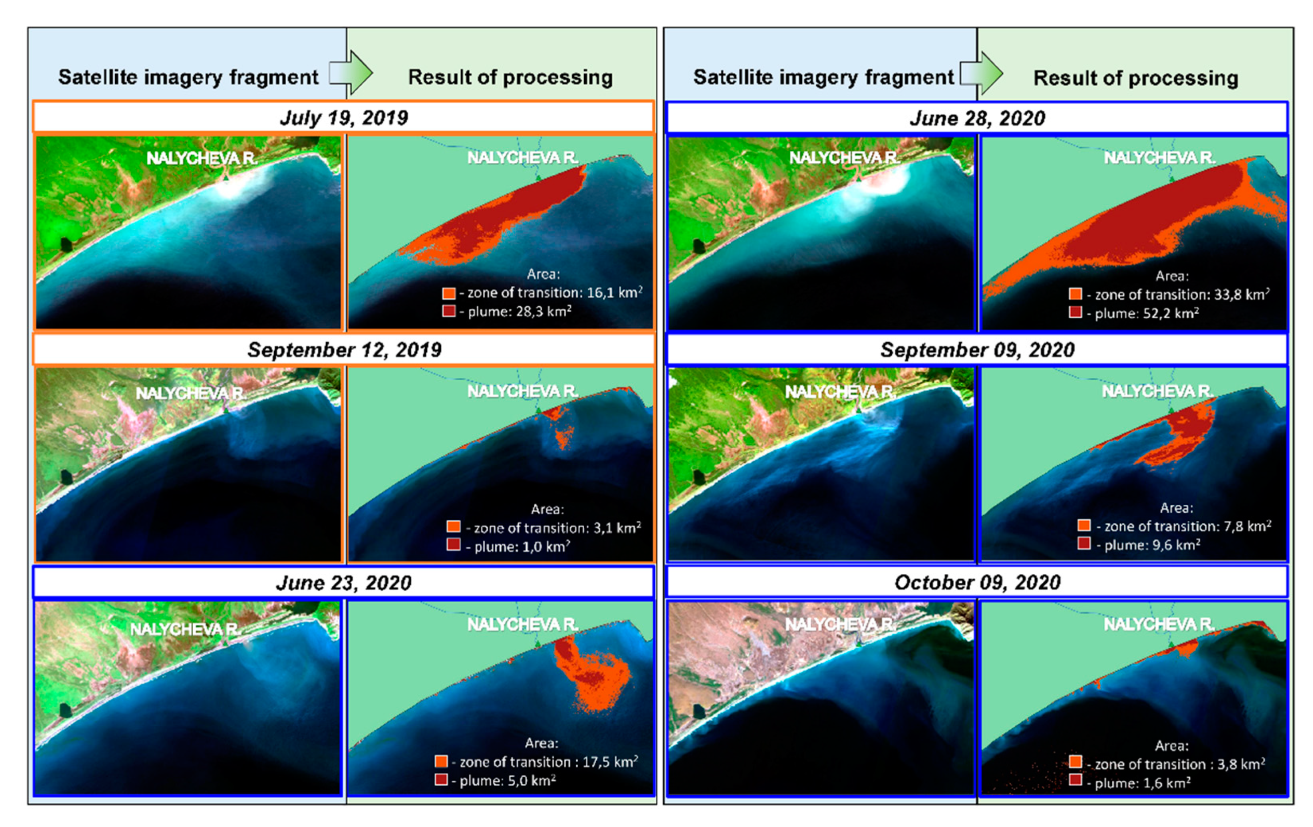
3.3. River Runoff (Sentinel-2A/B)

Optical multispectral satellite images obtained from the Sentinel-2A/B satellites on cloudless days of the summer-fall season of 2019 and 2020 near the mouth of the Nalycheva River were recalculated into TSM values in accordance with the method described above, and then processed using two thresholds. Threshold 1 assumed the selection of all pixels for which the TSM value exceeds 9 mg/m³, and made it possible to determine the distribution area of the “plume core” of waters carried by the Nalycheva River into the bay. Threshold 2 assumed the selection of all pixels for which the TSM value exceeded 5 mg/m³, but did not exceed the value of threshold 1, which made it possible to determine the boundaries of the “transition zone” of the plume [9,31]. The results of identifying the areas of distribution of plumes of the Nalycheva River runoffs in the Avacha Gulf are shown in Figure 9.

The analysis of Figure 9 has allowed us to note the following:

• The Nalycheva River runoff plume in 2019–2020 had a significant impact on the optical characteristics of the waters of the Avacha Gulf near the mouth of this river, which is reflected in an increase in the TSM concentration values determined by the C2RCC algorithm. The influence of runoff can be traced both in 2019 and in 2020.
• In 2019, the Nalycheva River runoff plume was reliably recorded two times (Figure 9 (images with an orange frame)), and in 2020 four times (Figure 9 (images with a blue frame)). In this case, the largest plume area (the combination of the “core” and the “transition zone”) in 2019 was ~44 km², while in 2020, the plume was recorded almost twice as large, amounting to ~86 km².
• Optical properties of waters entering the Avacha Gulf from the Nalycheva River, testified to the bringing suspensions containing nutrients of biological and mineral origins. Attention is drawn to the fact that this process in 2020 run much more intensively than in 2019.

Based on the data obtained and analyzed, it can be assumed that in 2020 the Nalycheva River runoff mode created conditions favorable to the development of HABs in the Avacha Gulf. It is noteworthy that the largest area of the Nalycheva River plume was recorded on 28 June 2020 (see Figure 9), with the strongest temperature anomaly recorded on 27 June 2020 (see Figure 6). An increase in temperature under normal light intensity and the sufficiency of nutrients entering the marine environment, including with river runoff, has a positive effect on the growth rate of algae and their photosynthesis. Thus, the release of a large amount of nutrients into the coastal water area and an anomalous increase in the temperature of the water environment that almost coincided with this event was a powerful factor in the accelerated development of microalgae. An analysis of Figure 8, illustrating the results of processing space radar images, also indicated that HAB developed most intensively directly in the area of the Nalycheva River mouth.

3.4. Validity of the Obtained Results

Let’s address the limitations of use of satellite oceanography data. In our research, first of all, we took into account the characteristics of information product accuracy declared by the developers, as well as the impact of weather (particularly, atmospheric) phenomena. For example, it is known that the accuracies of absolute chlorophyll-a concentration value retrieval using global algorithms according to MODIS spectroradiometer (Terra and Aqua satellites) data largely depend on the region of research (including on the water type and atmospheric aerosol types). Thus, the paper analyzes not individual absolute values of recorded parameters of the water environment but the entire available array of data on three types of significant parameters for the selected study area (SSH, 1993/2020; SST, 1982/2020; chlorophyll-a, 2000/2020).

This approach has allowed us to assess the dynamics of the measured significant parameters of the water area at the time of HAB preparation and development in Kamchatka in 2020 compared to the results of previous measurements. The comparative analysis addressed the mean values and standard deviations of the measured parameters, which are characteristic of the study area, recorded in a long historical retrospective (with the same instruments). At the same time, the features of the natural seasonal variation of the studied values were taken into account.

The validity of the outcome obtained is evidenced by the mutual correspondence of the results of detecting anomalies in the sea surface level, temperature, and concentration of chlorophyll-a obtained using different-type observation and data processing systems. For example, revealing the event of sharp increase of chlorophyll-a concentration was carried out using data from both VIIRS and MODIS spectroradiometers. At the same time, temperature anomalies registered based on long-term NOAA OISST data series processing are confirmed by MODIS data. The SSH HYCOM data processing results are supported with SLA AVISO data.

Control of possible errors of algorithms used to obtain the results is also to be noted. The graphs given in Figure 5, Figure 6 and Figure 7 were obtained using the technique programmed in Google Earth Engine and MS Excel environments and described in Section 2.2. To control possible errors in the development of the algorithm, verification calculations of the variation of the measured parameters (SST/NOAA, chlorophyll-a/MODIS) were carried out manually for several dates having the key importance for our effort. When compared with the results of automatic processing of the entire data set, no errors were found.

Figure 10 shows an essential graphs of annual variability of two registered key water environment parameters for the representative dates (annual time intervals) revealed in Section 3.1.2 and Section 3.1.3 (27 June SST; and September, chlorophyll-a) obtained as a result of verification calculations.

An analysis of the graphs given in Figure 10 allows us to see the deviations of the values of sea surface temperature (Figure 10, top) and chlorophyll-a (Figure 10, bottom) in 2020 relative to the set of measurement results performed in the historical retrospective. We can point out that the graphs shown in Figure 10 describe cases of registration of historical maxima of SST and chlorophyll-a. At the same time, the values of 2020 go quite far beyond the variability of the values of previous years, which corresponds to the results obtained in Section 3.2 and Section 3.3. The additional “Data Availability Statement” section contains links to the program codes of the Google Earth Engine, allowing us to obtain the data shown in Figure 10.

The accuracy, Δ, assessment was carried out for the selected examples. Confidence intervals, ±Δ, were calculated (see red segments in Figure 10). Let’s briefly ground the given accuracy values.

The NOAA OISST package includes a raster layer that characterizes the assessed SST error (standard deviation) for each pixel of daily information products [20]. The accuracy with a 95% confidence level was determined on account of the assumption of normal distribution:

$${\Delta }_{SST} ~ \overline{\sigma } · z_{0.95} ~ \overline{\sigma } · 1.96$$

(6)

where $\overline{\sigma }$ is the mean standard deviation of SST measurements within the studied site, z_0,95 is the quantile of a normal distribution for 95% confidence level.

C_{CHLOR_A} chlorophyll-a concentrations were measured repeatedly and then were averaged. In this case, the accuracy of the estimates obtained can be determined based on a priory known RMS of the algorithm that retrieves chlorophyll-a concentrations based on the measured spectral reflectance of the water surface. In the information product used in this effort, the values of chlorophyll-a concentration were obtained using the OC3M regression algorithm, while it is known that the RMS for Log10 (C_{CHLOR_A}) is 0.255 [36]. Taking into account the above, the accuracy of chlorophyll-a assessment on a logarithmic scale was determined as follows:

$${\Delta }_{LOG-CHLOR\_A} ~ \frac{RMS}{\sqrt{n}}·z_{0.95} ~ \frac{0.255}{\sqrt{\raisebox{1ex}{$n_{month-no-cloud}$}\!\left/ \!\raisebox{-1ex}{$n_{site}$}\right.}}·1.96$$

(7)

where n is the number of observations, defined as the ratio of the number of n_{month-no-cloud} cloudless pixels used in the calculation (equipment of the TERRA and AQUA satellites) to the area of the studied water area (n_site) expressed in a number of pixels. The limits of the ±Δ_{LOG-CHLOR_A} confidence interval calculated on a logarithmic scale were converted to the ±Δ_{CHLOR_A} linear representation and plotted. In addition, n «floor» values are shown in this graph (see Figure 10).

In the given example, the accuracy of the obtained SST values in percent varied between 2.1% and 16.1%, and the accuracy mean for the whole observation period was 7.1%. The accuracy of the obtained chlorophyll-a data in percent varied between 18.7% to 37.8%, and the accuracy mean for the whole observation period was 25.2%. Shown in Figure 10 confidence intervals indicate that the abnormally high values of SST and chlorophyll-a concentrations registered in 2020 exceed the values of possible errors of the analyzed information products.

In conclusion, we note that the fact of HABs in Kamchatka in September–October 2020 was confirmed by the results of field studies, which is recorded in the HEADAT international list of HABs [37]. The samples revealed a high concentration of toxic substances related to the poison causing DSP (diarrhetic shellfish poisoning). The main causative agents of such toxic substances are dinoflagellate algae of the Karenia species. The concentration of harmful algae, according to the HAEDAT information sheets, increased from 152,000 cells/L (4 October 2020) to 482,208 cells/L (12 October 2020) and up to 622,000 cells/L (13 October 2020).

4. Conclusions

The processing results for long-term retrospective series of daily satellite data on the sea surface height (since 1993) and temperature (since 1982) have allowed us to observe the preconditions of intensive harmful algal blooms in Kamchatka in the fall 2020. Registered ocean level variability in the 2020 summer months affected the current mode (predominantly anticyclonic vortexes were observed) and microalgae food resource formation. The strongest temperature anomalies of the water environment on record (reaching 6 °C in comparison with the climatic norm in June–July), combined with the specific conditions of the circulation of coastal waters, provided extremely favorable conditions for the seasonal development of phytoplankton, which ultimately led to an intense red tide and had a negative impact on the coastal waters of the Kamchatka Peninsula (up to the mass death of hydrobionts).

The harmful algal bloom that occurred in Kamchatka in the fall of 2020 was most clearly recorded in the form of an abnormal increase in the chlorophyll-a concentration in the coastal waters of the Kamchatka Peninsula compared to previous years (2000–2019). The monthly average value of this parameter in October 2020 (blooming peak) approached 15 mg/m³ what exceeds the climatic norm almost four-fold. At the same time, based on the results of space radar image interpretation, a large number of surface films of biogenic origin were recorded localized mainly near the coast, in the areas where rivers flow into the water area of the Avacha Gulf. During the study period (2019–2020), river runoff intensively introduced mineral and biogenic suspensions into the marine environment, expanding the food supply for microalgae (the values of total suspended matter within the Nalycheva River plume reached 10 mg/m³ or more in 2020).

The main novelty of this effort is the study and presentation of a specific, previously unused experimental setup for a comprehensive study of long-term retrospective series of heterogeneous information products of satellite oceanography to explain the causes and features of a single large-scale ecological disaster (i.e., the harmful algal bloom in Kamchatka which occurred in 2020). We can conclude that the final results are sufficiently valid taking into account the limitations of the data, methods, and approaches involved in the study, as well as the mutual correspondence of the results obtained on the basis of processing and analyzing information from various sources.

Other known events of intensive harmful algal blooms that had negative impacts on the ecosystems of marine areas can be studied using the suggested method, which allows one to process long-term retrospective series of satellite data on sea surface height and temperature, and chlorophyll-a concentration, as well as operative radar and optical imagery.

References

1. Anderson, D.M.; Glibert, P.M.; Burkholder, J.M. Harmful algal blooms and eutrophication: Nutrient sources, composition, and consequences. Estuaries 2002, 25, 704–726. [Google Scholar] [CrossRef]
2. Stumpf, R.P.; Tomlinson, M.C. Remote Sensing of Harmful Algal Blooms: Remote Sensing of Coastal Aquatic Environments; Springer: Dordrecht, The Netherlands, 2008; pp. 277–296. ISBN 978-1-4020-3099-4. [Google Scholar]
3. Cheng, W.; Hall, L.; Goldgof, D.; Soto, I.; Hu, C. Automatic Red Tide Detection from MODIS Satellite Images. In Proceedings of the IEEE International Conference on Systems, Man and Cybernetics, San Antonio, TX, USA, 11–14 October 2009; pp. 1864–1868. [Google Scholar]
4. Hu, C. A novel ocean color index to detect floating algae in the global oceans. Remote Sens. Environ. 2009, 113, 2118–2129. [Google Scholar] [CrossRef]
5. Wang, M.; Hu, C. Mapping and quantifying Sargassum distribution and coverage in the Central West Atlantic using MODIS observations. Remote Sens. Environ. 2016, 183, 350–367. [Google Scholar] [CrossRef]
6. Bondur, V.G. Satellite Monitoring and Mathematical Modelling of Deep Runoff Turbulent Jets in Coastal Water Areas. In Waste Water-Evaluation and Management; InTech: Rijeka, Croatia, 2011; pp. 155–180. ISBN 978-953-307-233-3. [Google Scholar]
7. Bakhtiar, M.; Rezaee Mazyak, A.; Khosravi, M. Ocean Circulation to Blame for Red Tide Outbreak in the Persian Gulf and the Sea of Oman. IJMT 2020, 13, 31–39. [Google Scholar]
8. Zhao, J.; Ghedira, H. Monitoring red tide with satellite imagery and numerical models: A case study in the Arabian Gulf. Mar. Pollut. Bull. 2014, 79, 305–313. [Google Scholar] [CrossRef]
9. Bondur, V.G.; Zamshin, V.V.; Chvertkova, O.I. Space Study of a Red Tide-Related Ecological Event near Kamchatka Peninsula in September–October 2020. Dokl. Earth Sci. 2021, 497, 255–260. [Google Scholar] [CrossRef]
10. Binding, C.E.; Greenberg, T.A.; McCullough, G.; Watson, S.B.; Page, E. An Analysis of Satellite-Derived Chlorophyll and Algal Bloom Indices on Lake Winnipeg. J. Great Lakes Res. 2018, 44, 436–446. [Google Scholar] [CrossRef]
11. Ahn, Y.H.; Shanmugam, P. Detecting the red tide algal blooms from satellite ocean color observations in optically complex Northeast-Asia Coastal waters. Remote Sens. Environ. 2006, 103, 419–437. [Google Scholar] [CrossRef]
12. Lou, X.; Hu, C. Diurnal changes of a harmful algal bloom in the East China Sea: Observations from GOCI. Remote Sens. Environ. 2014, 140, 562–572. [Google Scholar] [CrossRef]
13. Sakamoto, S.; Lim, W.A.; Lu, D.; Dai, X.; Orlova, T.; Iwataki, M. Harmful algal blooms and associated fisheries damage in East Asia: Current status and trends in China, Japan, Korea and Russia. Harmful Algae 2021, 102, 101787. [Google Scholar] [CrossRef] [PubMed]
14. Sukhanova, I.N.; Flint, M.V. Anomalous blooming of coccolithophorids over the eastern Bering Sea shelf. Oceanology 1998, 38, 502–505. [Google Scholar]
15. Bondur, V.G.; Grebenyuk, Y.u.V.; Sabinin, K.D. Peculiarities of internal tidal wave generation near Oahu Island (Hawaii). Oceanology 2009, 49, 299–309. [Google Scholar] [CrossRef]
16. Shi, W.; Wang, M. Observations of a Hurricane Katrina-induced phytoplankton bloom in the Gulf of Mexico. Geophys. Res. Lett. 2007, 34, L11607. [Google Scholar] [CrossRef]
17. Wang, M.; Lide, J.; Xiaoming, L.; Karlis, M. Satellite-derived global chlorophyll-a anomaly products. Int. J. Appl. Earth Obs. Geoinf. 2021, 97, 102288. [Google Scholar] [CrossRef]
18. Luchin, V.A.; Kruts, A.A. Properties of cores of the water masses in the Okhotsk Sea. Izv. TINRO 2016, 184, 204–218. [Google Scholar] [CrossRef]
19. Chassignet, E.; Hurlburt, H.; Metzger, E.; Smedstad, O.; Cummings, J.; Halliwell, G.; Bleck, R.; Baraille, R.; Wallcraft, A.; Lozano, C.; et al. Global Ocean Prediction with the Hybrid Coordinate Ocean Model (HYCOM). Oceanography 2009, 22, 64–75. [Google Scholar] [CrossRef]
20. Reynolds, R.W.; Banzon, V.F.; NOAA CDR Program. NOAA Optimum Interpolation 1/4 Degree Daily Sea Surface Temperature (OISST) Analysis, Version 2. NOAA Natl. Cent. Environ. Inf. 2008. [Google Scholar] [CrossRef]
21. LAS (Live Access Server): Aviso+. Available online: https://www.aviso.altimetry.fr/en/data/data-access/las-live-access-server.html (accessed on 1 February 2021).
22. ESA European Space Agency—Missions—Sentinel-2. Available online: https://sentinel.esa.int/web/sentinel/missions/sentinel-2 (accessed on 13 May 2021).
23. ESA European Space Agency—Missions—Sentinel-1. Available online: https://sentinels.copernicus.eu/web/sentinel/missions/sentinel-1 (accessed on 13 May 2021).
24. NASA Goddard Space Flight Center, Ocean Ecology Laboratory, Ocean Biology Processing Group. Moderate-Resolution Imaging Spectroradiometer (MODIS). Available online: https://modis.gsfc.nasa.gov/ (accessed on 13 May 2021).
25. NASA Goddard Space Flight Center, Ocean Ecology Laboratory, Ocean Biology Processing Group. Visible and Infrared Imager/Radiometer Suite (VIIRS). Available online: https://www.nasa.gov/mission_pages/NPP/mission_overview/index.html (accessed on 13 May 2021).
26. Bondur, V.G.; Grebenyuk, Y.V.; Sabynin, K.D. The spectral characteristics and kinematics of short-period internal waves on the Hawaiian shelf. Izv. Atmos. Ocean. Phys. 2009, 45, 598–607. [Google Scholar] [CrossRef]
27. Ivanov, A.Y. Slicks and Oil Films Signatures on Syntetic Aperture Radar Images. Issled. Zemli Iz Kosm. 2007, 3, 73–96. [Google Scholar]
28. Erokhin, V.E.; Gordienko, A.P. Influence of organic pollutants on the growth of dinophytic microalgae. Issues Mod. Algol. 2019, 21, 48–55. [Google Scholar] [CrossRef]
29. Brockmann, C.; Doerffer, R.; Peters, M.; Kerstin, S.; Embacher, S.; Ruescas, A. Evolution of the C2RCC Neural Network for Sentinel 2 and 3 for the Retrieval of Ocean Colour Products in Normal and Extreme Optically Complex Waters. In Proceedings of the Living Planet Symposium (ESA SP-740, August 2016), Prague, Czech Republic, 9–13 May 2016; p. 54. [Google Scholar]
30. Pugach, S.P.; Pipko, I.I.; Shakhova, N.E.; Shirshin, E.A.; Perminova, I.V.; Gustafsson, O.; Bondur, V.G.; Ruban, A.S.; Semiletov, I.P. Dissolved organic matter and its optical characteristics in the Laptev and East Siberian seas: Spatial distribution and interannual variability (2003–2011). Ocean. Sci. 2018, 14, 87–103. [Google Scholar] [CrossRef] [Green Version]
31. Bondur, V.G.; Vorobjev, V.E.; Grebenjuk, Y.V.; Sabinin, K.D.; Serebryany, A.N. Study of fields of currents and pollution of the coastal waters on the Gelendzhik Shelf of the Black Sea with space data. Izv. Atmos. Ocean. Phys. 2013, 49, 886–896. [Google Scholar] [CrossRef]
32. Filimonov, V.S.; Aponasenko, A.D. Seasonal dynamics of suspended matter in waters of lake Khanka. Atmos. Ocean. Opt. 2013, 26, 524–531. [Google Scholar] [CrossRef]
33. Vakulskaya, N.M.; Dubina, V.A.; Plotnikov, V.V. Eddy structure of the East Kamchatka current according to satellite observations. Phys. Geosph. 2019, 1, 73–81. [Google Scholar] [CrossRef]
34. Andreev, A.G. Water circulation in the north-western Bering sea studied by satellite data. Issled. Zemli Iz Kosm. 2019, 4, 40–47. [Google Scholar] [CrossRef]
35. Mikaelyan, A.S.; Zatsepin, A.G.; Kubryakov, A.A. Effect of Mesoscale Eddy Dynamics on Bioproductivity of the Marine Ecosystems (Review). Phys. Oceanogr. 2020, 27, 590–618. [Google Scholar] [CrossRef]
36. Chlorophyll-a (Chlor-a) ATBD. Available online: https://oceancolor.gsfc.nasa.gov/atbd/chlor_a/ (accessed on 29 September 2021).
37. Harmful Algal Event Database. Available online: http://haedat.iode.org/ (accessed on 20 January 2021).
38. Google Earth Engine Code (Chlorophyll-a Key Anomaly). Available online: https://code.earthengine.google.com/0401cac5c4a3cfcffed3501a08c98a36 (accessed on 20 August 2021).
39. Google Earth Engine Code (SST Key Anomaly). Available online: https://code.earthengine.google.com/40ab28733e0347cd56674612f1c8369d (accessed on 20 August 2021).
Figure 1. Schematic map of the study area with the locations of registration of negative harmful algal bloom indicators registered near the Kamchatka shore in the fall of 2020.
Jmse 09 01092 g001
Figure 2. Flowchart of the experiment for processing of long-term retrospective series of satellite data on the ocean level, sea surface temperature, and chlorophyll-a concentration.
Jmse 09 01092 g002
Figure 3. Flowchart of the experiment for processing Sentinel-1A/B radar satellite imagery.
Jmse 09 01092 g003
Figure 4. Flowchart of the experiment for processing Sentinel-2A/B multispectral imagery.
Jmse 09 01092 g004
Figure 5. The graphs characterizing the annual variation of daily SSH (sea surface height) values for 2020 (red line) and summarized for the period from 1993 to 2019. SSH values (black line denotes average values, dashed lines denote standard deviations) characterizing the climatic norm (based on HYCOM data processing). The insets show spatial distributions of sea level anomalies and directions of geostrophic currents for the dates of registration of the anomalous sea level: 19 April, 3 Jun, 30 August, 15 September, 19 September (Aviso + data, 2020).
Jmse 09 01092 g005
Figure 6. Graphs characterizing the annual variation of daily SST (sea surface temperature) values for 2020 (red line) and summarized for the period from 1981 to 2019 SST values (black line denotes average values, dashed lines denote standard deviations) based on NOAA OISST data processing. The insets (ad) based on MODIS data show spatial distributions of SST on 22, 27 June and 24, 27 July (when the most intensive anomalies had been formed).
Jmse 09 01092 g006
Figure 7. Information products formed during the assessment of phytoplankton bloom intensity in the Avacha Gulf: daily spatial distributions of chlorophyll-a concentration (in conv. units) in September–October 2020, obtained from the processing of VIIRS data (NOAA satellites) (above); the graphs characterizing the monthly average values of chlorophyll-a concentrations from May to October 2020 (red line), as well as from May to October averaged over the time period from 2000 to 2019. (blue line denotes average values, dashed lines denote standard deviation) characterizing the climatic norm (obtained from MODIS data processing (AQUA and TERRA satellites).
Jmse 09 01092 g007
Figure 8. Radar satellite image interpretation result (Sentinel-1A/B) (the images were obtained between 25 August and 5 October 2020). The map of zones of increased accumulation of biogenic surfactants in the Avacha Gulf (left). Right, the map of chlorophyll-a concentration distribution (NOAA VIIRS) averaged over the period from 25 August to 5 October 2020.
Jmse 09 01092 g008
Figure 9. Maps of the Nalycheva river plume propagation areal in 2019 and 2020 (Sentinel-2A/B, TSM concentration spatial distribution thresholding, the plume’s “core” and “transition zone” are identified).
Jmse 09 01092 g009
Figure 10. Annual variability of parameters averaged over the area of the study region: top, 27 June SST daily values for 1982–2020; bottom, September chlorophyll-a monthly values for 2000–2020. Red segments denote confidence intervals (95%).
Jmse 09 01092 g010aJmse 09 01092 g010b
Publisher’s Note: MDPI stays neutral with regard to jurisdictional claims in published maps and institutional affiliations.