Liquid–Solid Flow Characteristics in Vertical Swirling Hydraulic Transportation with Tangential Jet Inlet

Abstract

In order to improve the efficiency and safety of vertical hydraulic transport systems for non-spherical particles, a new pipeline transport system with a tangential jet inlet is adopted in this study, and a modified non-spherical drag coefficient model is used to analyze the liquid–solid flow characteristics based on the CFD-DEM (Computational Fluid Dynamics-Discrete Element Method) coupling method. The focus of the study is on the influence of different tangential flow proportions in terms of the velocity distribution, the vorticity, the total pressure, the concentration and drag force of particles of various shapes. The conveying efficiency is measured according to the fluid velocity distribution and the particle concentration, and the safety of conveying is evaluated according to the flow structure and drag force of the particles. The result shows that the velocity of the swirling pipes is significantly higher than the straight pipe. With the increase of the tangential flow proportion, the swirling number and the vorticity magnitude increase, and the vortex core is broken and merged more quickly. Furthermore, the concentration gap and axial drag force gap between particles of various shapes are reduced with the effect of swirling flow, the particle concentration increases, and the particles of each component are uniformly mixed and transported.

1. Introduction

In recent years, the rapid development of the industry makes terrestrial mineral resources increasingly exhausted. In order to meet the needs of industrial development, countries around the world have turned their attention to the seabed mineral resources that have not been systematically developed and have upgraded the development of seabed mineral resources to national strategic objectives [1]. In the deep-sea mining system, a common transportation method is pipeline hydraulic lifting, which is a transportation method of conveying materials through pipelines with liquid (usually water) as the carrier. Due to its advantages of pollution-free, energy-saving, weather-free and large transportation volume, it is widely used in ocean engineering fields, such as submarine oil lifting [2]. However, in deep-sea hydraulic transportation, the transportation of ore is limited by the unique working conditions. The precious minerals contained in the seafloor of several thousand meters are in the category of coarse particles. The larger particle size and irregular shape mean that the technology for lifting the ore from the seafloor to the mining vessel is extremely complex and important [3,4]. At present, deep-sea mining technology has not yet reached the requirements of large-scale commercial mining, but the current research on deep-sea mineral transportation shows that vertical pipeline hydraulic transportation is most likely to become the first-generation commercial implementation scheme [1].

At present, scholars have conducted a lot of research on the mechanism of vertical pipeline hydraulic transportation. Durand [5] studied the critical flow under the experimental condition of particle size D = 0.44~2.04 mm. Xu et al. [6] analyzed the momentum transfer of particles and carriers in horizontal pipelines and proposed a new heterogeneous velocity distribution model. Asakura et al. [7] numerically simulated the hydraulic lifting process of glass beads with a diameter of 2 mm in the vertical pipe. Xia et al. [8] adopted a new research method for the hydraulic gradient of the mixed flow under different flow and particle load conditions. Souza et al. [9] conducted pumping experiments on particles of multi-component ore with a diameter of 0.2 mm and analyzed data of different concentrations and speeds. Among the current research on liquid–solid two-phase flow characteristics, there are many studies on horizontal pipes and fine particles, while there are few studies on vertical pipes and coarse particles. The motion state of coarse particles in the pipeline is more complex than that of fine particles, and it will face new problems in the vertical pipe. Therefore, it is of great significance to study the solid–liquid two-phase flow characteristics of coarse particle transportation in vertical pipelines.

Currently, the transportation of coarse particles is becoming more and more common in the field of industrial transportation, while the application and research of traditional axial flow transportation are mainly suitable for fine particles. To solve this dilemma, many scholars have conducted research on optimized flow structure. Li and Tomita [10,11] studied the swirling pneumatic conveying system of particles with different sizes. The research shows that the pressure loss, energy consumption and minimum conveying speed of the swirl pneumatic conveying system are significantly lower than those of the axial flow system in horizontal pipes. Fokeer et al. [12,13] and Zhou et al. [14] studied the velocity distribution of the swirling field of the three-lobed pipe, the rifling pipe and the guide vane pipe, and found the variation and attenuation of the swirling flow. Rinoshika [15] and Yan et al. [16] proposed the study of oscillating flow pneumatic conveying using a built-in soft rib, and found that, compared with axial flow conveying, the wind speed, pressure drop and energy consumption coefficient can be significantly reduced. Yin et al. [17] conducted a study on the swirling hydraulic transport of vertical pipes and found that swirling flow has an enrichment effect on particles and increases the kinetic energy of particles. However, the current flow structure improvement is mostly based on the horizontal pipe, and there are few studies on the vertical pipe, so it is extremely important to optimize the flow structure of the vertical pipe. At the same time, the above-mentioned studies give less consideration to the particle shape, and the coarse non-spherical particles are extremely sensitive to the change of the flow structure in the pipe, so the particle shape needs to be discussed.

At present, the study of non-spherical particles includes two parts: drag coefficient model modification and particle discrete element modeling, and the common method of forming non-spherical particles is spherical element filling method. Zhong et al. [18] used the spherical element filling method to generate cylindrical particles and selected the drag coefficient model proposed by Tran-Cong et al. [19] to study the cylindrical particle fluidized bed, and the results were in agreement with the experimental data. Ren et al. [20] established a non-spherical drag model by themselves, considering factors such as particle orientation and density difference, and the calculated results of cylindrical particles were in good agreement with the experimental results. Molaei et al. [21] used the non-spherical drag coefficient formula proposed by Hölzer and Sommerfeld [22] in the study of the ellipsoidal hydraulic fluidized bed, and the fluidization effect is obvious. The movement of non-spherical particles in the flow field is extremely complex. The particle shape considered in the current research is relatively simple, and there are few studies on the mixed flow of multi-component particles. In order to further push the numerical calculation of vertical hydraulic ore migration to the actual results, the various forms of particles are modeled and are then based on CFD-DEM; it is very important to use the appropriate non-spherical resistance coefficient formula to study the mixed transportation of multi-component particles.

In this paper, a new pipeline transportation system is proposed, which has three tangential inlets based on Archimedes spirals. The flow structure is changed by the intersection of tangential jet and mainstream to solve the low transportation concentration, low particle starting velocity and easy blockage at the initial section of the pipeline. It is worth mentioning that in the current research on particle flow, some scholars have adopted the CFD-DEM calculation method. However, most of the simulation is based on the software built-in model, which greatly affects the accuracy and authenticity of the study. Therefore, the CFD-DEM method is used for coupling calculation, and the built-in drag force model of the software interface is modified to ensure the calculation accuracy of non-spherical particles. Under the conditions of different tangential proportions and different particle shapes, the multi-component and multi-scale research on the characteristics of solid–liquid two-phase flow is carried out in terms of the fluid velocity distribution, the flow vorticity, the pressure distribution, the particle motion state and the drag force on particles.

2. Methodologies

2.1. Governing Equation of the Liquid and Solid Phase

In this paper, the Euler–Lagrangian framework was adopted, and the liquid and solid phase models were considered separately based on the CFD-DEM coupling method. The fluid velocity of the fluid transportation conditions studied in this paper is much lower than the speed of sound, and the heat exchange between the phases can be ignored during the transportation process. Therefore, only the liquid-phase governing equations need to be selected from the aspects of mass conservation and momentum conservation.

The continuous phase liquid-phase flow was controlled by Navier–Stokes equation [13,17]:

$$\frac{\partial \alpha {\rho }_l}{\partial t}+\nabla \cdot {\rho }_l\alpha U_l=0$$

(1)

$$\frac{\partial \alpha {\rho }_l{U}_l}{\partial t}+\nabla \cdot {\rho }_l\alpha U_l\otimes U_l=-\nabla \cdot p+\nabla \cdot ({\mu }_l\alpha \nabla U_l)+{\rho }_l\alpha g-F_w$$

(2)

where ${\rho }_l$ is the fluid density, $U_l$ is the fluid velocity, t is the time, μ_l is the fluid viscosity, g is the gravitational acceleration, α is the void ratio and p is the pressure. F_w is the transfer quantity of liquid–solid phase:

$$F_w=F_{drag}+F_{Magnus}+F_{Saffman}$$

(3)

The realizable k-ε turbulence model is a supplement to the standard k-ε model, which was proposed by Shih [23]. The model is basically consistent with the RNG (Renormalization group) k-ε model, but the vortex viscosity calculation is improved, and a new equation is proposed. The advantage of the realizable k-ε turbulence model is that it cannot only describe the swirling flow, but also simulate the cylindrical jet very well, such as predicting the propagation velocity of the symmetric jet, which is very suitable for the research conditions in this paper. The governing equation of the realizable k-ε turbulence model is described by:

$$\frac{\partial }{\partial t}({\rho }_{l}k)+\frac{\partial }{\partial x_i}({\rho }_{l}k{u}_l)=\frac{\partial }{\partial x_j}\left(\left({\mu }_l+\frac{{\mu }_t}{{\sigma }_k}\right)\frac{\partial k}{\partial x_j}\right)+G_k-{\rho }_l\epsilon$$

(4)

$$\frac{\partial }{\partial t}({\rho }_l\epsilon )+\frac{\partial }{\partial x_i}({\rho }_l\epsilon u_l)=\frac{\partial }{\partial x_j}\left(\left(\mu +\frac{{\mu }_t}{{\sigma }_{\epsilon }}\right)\frac{\partial \epsilon }{\partial x_j}\right)+{\rho }_l{C}_{1}E\epsilon -{\rho }_l{C}_2\frac{{\epsilon }^2}{k+\sqrt{v_l\epsilon }}$$

(5)

where k represents the turbulent kinetic energy and ε represents the turbulent dissipation rate. σ_k, σ_ε are the Prandtl numbers corresponding to k and ε, σ_k and σ_ε are 1 and 1.2, respectively. C₁ and C₂ are constants, C₁ is 1.44 and C₂ is 1.9. μ_l is the liquid velocity and v_l is the kinematic viscosity coefficient [23,24].

In order to describe the translational and rotational motion of particles, Newton’s law of motion is adopted [25]:

$$m_p\frac{d{U}_p}{dt}=F_{drag}+F_{Saffman}+F_{Magnus}+F_c+m_{p}g$$

(6)

$$I_P\frac{d{\omega }_p}{dt}=T_p$$

(7)

where m_p, I_p, T_p, U_p, ω_p are the mass, the moment of inertia, the moment, the translational velocity, rotational velocity of the particle, respectively. Fc is the collision force of particle-particle and particle-wall, controlled by the soft-sphere contact model.

Drag force is a parameter that determines the momentum exchange between liquid-phase and solid-phase, which directly affects the movement of particles. To calculate the drag force of each single particle and account for the effects of surrounding particles, the Di Felice [26] drag model is used, which is described by:

$$\{\begin{array}{l}{F}_{freestream}=0.5C_D{\rho }_l{A}_p(U_l-U_p)\left|U_l-U_p\right|\\ F_D=F_{freestream}{\epsilon }^{-(\chi +1)}\\ C_D={(0.63+\frac{4.8}{{\mathrm{Re}}^{0.5}})}^2\end{array}$$

(8)

where, C_D is the drag coefficient, A_p is the cross-sectional area of particle. χ is a correction factor accounting for crowding effects, which is calculated by the Reynolds number:

$$\chi =3.7-0.65\exp \left[-\frac{{(1.5-{\log }_{10}\mathrm{Re})}^2}{2}\right]$$

(9)

The Di Felice model is suitable for spherical particles, while the non-spherical particles are discussed in this paper. It is not accurate to describe non-spherical particles by spherical drag coefficient formula, so other non-spherical drag coefficient models are needed. According to the comparison of Bagheri and Bonadonna [27] on the accuracy of several existing non-spherical drag coefficient models, the drag coefficient model is selected as the Holzer and Sommerfeld [22] non-spherical model with higher accuracy. The drag coefficient is proposed based on a large number of experimental data and simulation data, so it is suitable for a wide range of Reynolds numbers. An important advantage of this coefficient is that it takes the influence of particle shape and direction into consideration, and the reliability of the formula has been proved by Hilton et al. [28], Zhou et al. [29] and Rong et al. [30]. The equation is expressed as:

$$C_D=\frac{8}{\mathrm{Re}}\frac{1}{\sqrt{{\mathsf{\Phi }}_{\perp }}}+\frac{16}{\mathrm{Re}}\frac{1}{\sqrt{\mathsf{\Phi }}}+\frac{3}{\sqrt{\mathrm{Re}}}\frac{1}{{\mathsf{\Phi }}^{3/4}}+0.42\times {10}^{0.4{(-{\log }^{\mathsf{\Phi }})}^{0.2}}\frac{1}{{\mathsf{\Phi }}_{\perp }}$$

(10)

where Φ and Φ_⊥ is the sphericity and crosswise sphericity, respectively. Φ_⊥ is defined as the ratio of the cross-sectional area of the volume equivalent sphere particle to the cross-sectional area of the considered particle.

Compared with the drag force, the Magnus force and Saffman force in this study are very small, and Tsuji et al. [31], Karimi and Dehkordi [32] have made a detailed description of this.

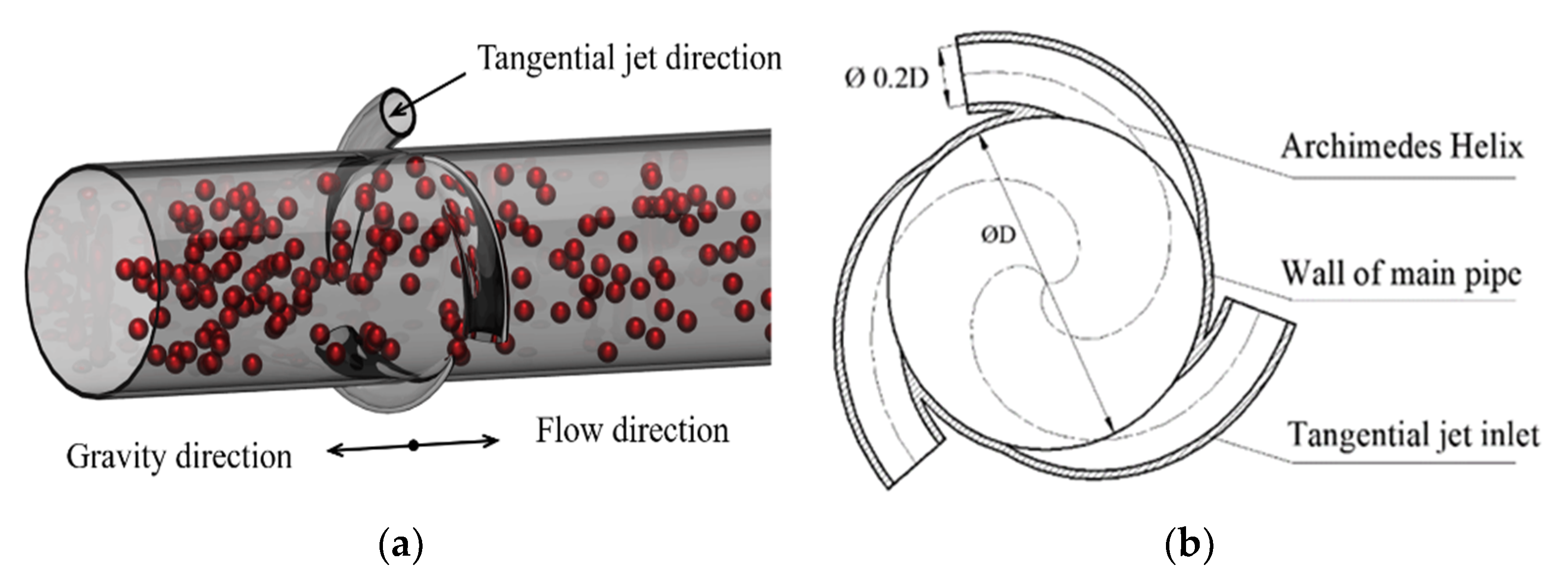
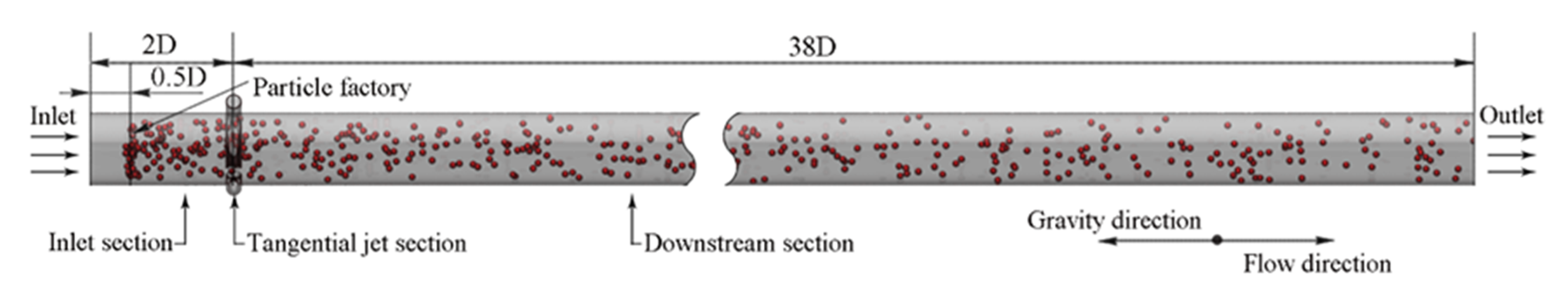
2.2. Simulation Modeling

There are two kinds of pipes analyzed in this study, one is straight pipe and the other is straight pipe with tangential jet inlet. The tangential jet inlet is a circular pipe, which extends along Archimedes helix and intersects with the main pipe. Figure 1a is spatial structure of the pipeline with a tangential inlet, and Figure 1b is the plane distribution of the tangential inlet. Different working conditions are abbreviated as TP30, TP20, TP10 and STP according to the proportion of tangential flow. The flow rate distribution is shown in

Table 1. Working condition codes for all cases.

Working Condition	Velocity of Main Pipe (m/s)	Velocity of Tangential Inlet (m/s)	Code
Tangential flow accounts for 10%	2.7	2.5	TP10
Tangential flow accounts for 20%	2.4	5	TP20
Tangential flow accounts for 30%	2.1	7.5	TP30
No tangential flow	3	0	STP

. Meanwhile, TP30, TP20, TP10 are collectively referred to as a swirling pipe, STP is collectively referred to as a straight pipe. Figure 2 is the schematic diagram of the conveying process of the swirling pipe. It can be seen that the calculation model is divided into three different calculation areas: inlet section, tangential jet section and downstream section.

The grids of different computing domains were divided separately, and the different grid areas were connected by an interface to transmit data. The inlet section and downstream section, which account for a large proportion of the entire computational domain, were divided by hexahedral structured grids, and the tangential jet section was divided by tetrahedral unstructured grids. In this study, two mesh sizes were used for liquid-phase calculation and loading calculation, respectively. The fine grid was used for liquid-phase calculation, as shown in Figure 3. The grid segments near boundary were refined and the standard wall function was used to calculate the flow of the near-wall region. When calculating the load particle condition, there is no need to pay attention to the flow of the near-wall region. Moreover, in order to ensure the accurate transfer of the momentum sink, the volume of the fluid phase grid needs to be greater than the particle volume, so 1.5 times the particle size is used for grid division to ensure calculation accuracy.

In order to analyze the flow structure of non-spherical particles in the flow field, in addition to spherical particles, three kinds of non-spherical particles were constructed by spherical element filling method. They are ellipsoidal, cylindrical and tetrahedral, and the volume of particles of various shapes is the same. Considering the calculation time period, the particles do not fully fit with the regular geometric shape, so the sphericity of the particles constructed is larger than that of the regular geometric shape, but this is more in line with the shape of the particles in the actual transportation process. The shape parameters of each particle are shown in

Table 2. Parameters of particles.

Particle Shape	DEM Model	Number of Filled Spheres	deq/mm	Φ
Sphere		1	20	1
Ellipsoid		5	20	0.9806
Cylinder		5	20	0.9123
Tetrahedron		10	20	0.9765

.

The CFD-DEM coupling process is a transient bidirectional data transfer process. Firstly, Fluent calculates the flow field information at a certain time step, and then EDEM (Discrete Element Simulation Software) performs the calculation. The position, movement, volume and other information of particles were transmitted to Fluent through the coupling interface to calculate the interaction between the particles-phase and liquid-phase. Then the effect of fluid on particles is transmitted through the interface to EDEM as the particle volume force, such as drag force, which affects the movement of particles. After the calculation of EDEM, the interphase force and volume fraction are returned to the CFD (Computational Fluid Dynamics) solver in the form of a momentum sink. Subsequently, a new round of calculation begins, and the whole process of transient simulation is realized by gradually circulating iteration.

In the CFD calculation, the solver based on pressure was selected because the flow in this study belongs to incompressible flow, the calculation mode was set to transient calculation and the realizable k-ε turbulence model was selected. The standard wall function, which ensures the calculation accuracy and makes the grid number at a reasonable level, was selected to calculate the near-wall flow. The governing equations were discretized by a finite volume method and the SIMPLE algorithm (Flow solving algorithm) was used for pressure–velocity coupling. The QUICK (The Quadratic Upstream Interpolation for Convective Kinematics) scheme improves the truncation error of the discrete equations and reduces the pseudo-diffusion error. The convection term of the QUICK scheme has the third-order truncation error, and the diffusion term has the second-order truncation error, which means high accuracy. Therefore, the QUICK discrete scheme is selected to solve the momentum and turbulence equations. In addition, when setting the boundary conditions, the main flow inlet and the three tangential jet inlets were set as the velocity inlet, the outlet was set as the pressure outlet (0 Pa) and the rest were set as no-slip walls.

In the CFD-DEM coupling calculation, the Eulerian–Lagrangian model was selected for coupling control, the drag force model was the Di Felice (1994) model, the drag coefficient formula was modified to the non-spherical formula proposed by Hölzer and Sommerfeld (2008), and the Saffman lift and Magnus lift were considered in the calculation. The remaining simulation parameters selected in this paper were shown in

Table 3. Parameters of simulation.

Phase	Item	Details	Index	Unit	Value
CFD	Materials	Fluid/water	Density	kg·m−3	1025
			Viscosity	kg·m−1·s−1	1.003 × 10−3
	Boundary conditions	Pressure outlet	Gauge pressure	Pa	0
		Wall	Wall motion		Stationary wall
			Shear condition		No slip
DEM	Materials	Particle	Poisson’s ratio	-	0.25
			Shear modulus	Pa	1 × 108
			Density	kg·m−3	2040
		Wall	Poisson’s ratio	-	0.3
			Shear modulus	Pa	7 × 1010
			Density	kg·m−3	7800
	Interaction	Particle–particle	Coefficient of restitution	-	0.525
			Coefficient of static friction	-	0.642
			Coefficient of rolling friction		0.05
			Interaction contact model		Hertz–Mindlin (no slip)
			Collision model		Soft-sphere contact model
		Particle-wall	Coefficient of restitution	-	0.525
			Coefficient of static friction	-	0.4
			Coefficient of rolling friction	-	0.05
			Interaction contact model		Hertz–Mindlin (no slip)
			Collision model		Soft-sphere contact model
	Particle	Particle factory	Particle radius	mm	20
			Factory type		Dynamic/unlimited number
			Target mass	kg/s	4

.

2.3. Model Validation

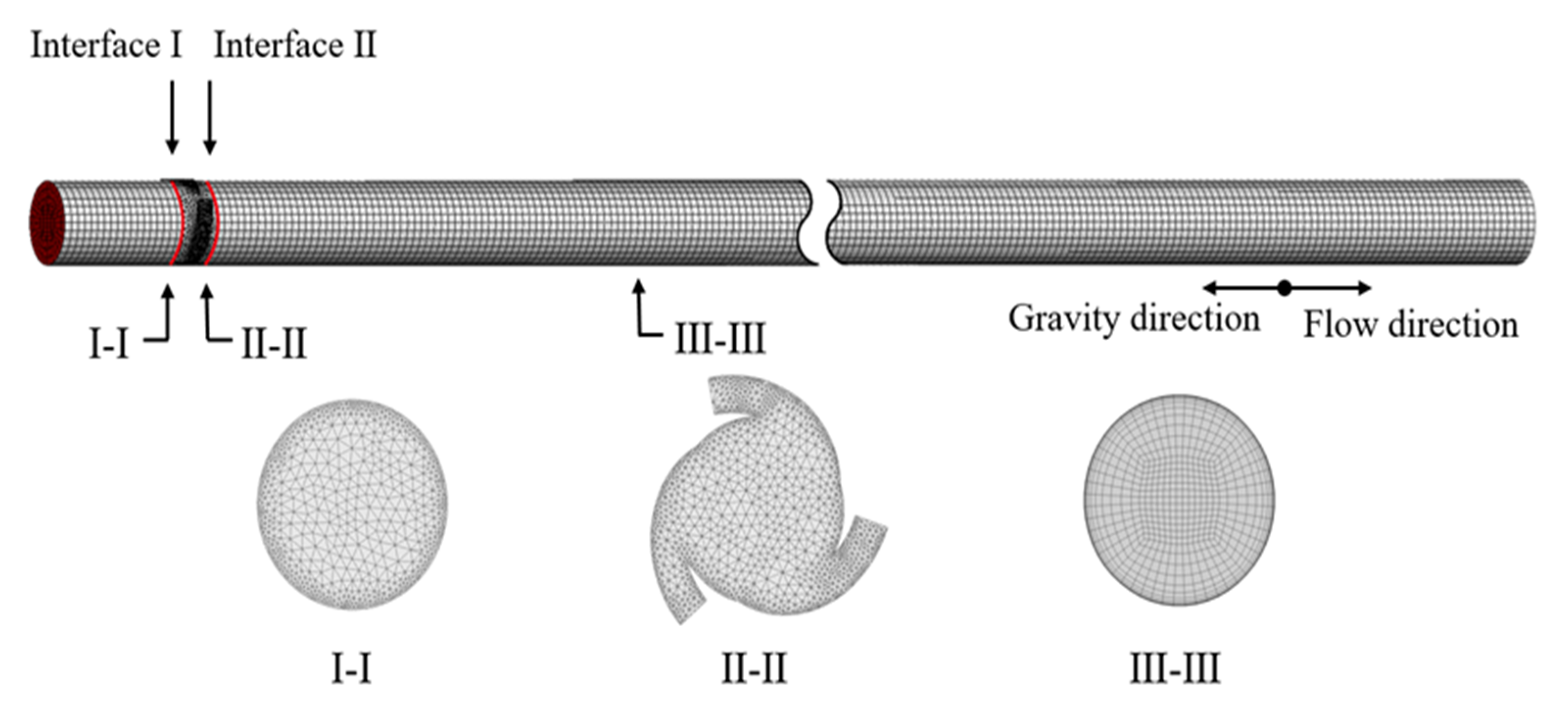
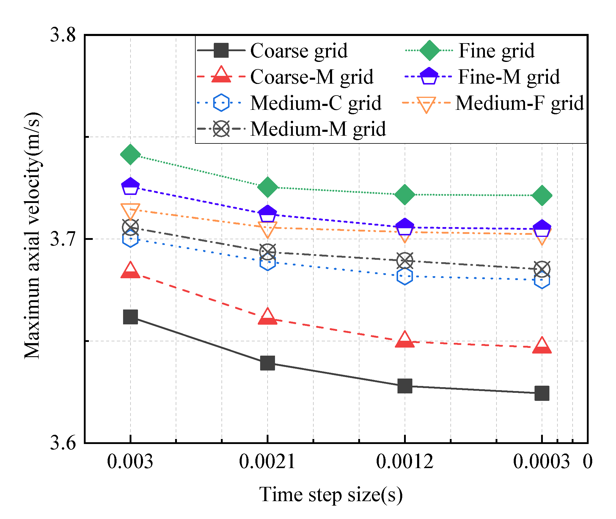
2.3.1. Grid Size Independence Tests

In order to verify the accuracy of the model, the simulation model was verified by grid size independence and time step independence. The computational domain was divided into four different mesh sizes, and four different time steps were used for the CFD numerical calculation. In the CFD-DEM coupling calculation, the time step of CFD was generally taken between 10 and 100 times of the time step of DEM, so the time step of CFD calculation in this verification was set to 0.003 s, 0.0021 s, 0.0012 s and 0.0003 s. The maximum number of iterations per time step was 30, the total simulation time for each case was set to 9 s, and the convergence residual standard is set to 1 × 10⁻⁵.

In order to make the number of grids at a reasonable level, instead of generating multi-layer dense grids at the near-wall region, the standard wall function is used to calculate the flow of the near-wall region in this paper. In this way, we are only arranging the necessary nodes of the first layer of the grid in the log-Law layer, that is, the range of $y^{+}$ is 30–300 [33]. Firstly, the first-layer grid height was estimated by Equation (11) [34], and then the actual value of $y^{+}$ was checked to meet the requirements after meshing and numerical calculation.

$$y^{+}=0.172\frac{\Delta y}{L}{\mathrm{Re}}_L^{0.9}$$

(11)

where ∆y is the first-layer grid height, L is the reference length.

Hence, when performing meshing, $y^{+}$ was initially set to 40. The first layer height was 0.0003 m, and the grid amplification ratio was 1.2.

Table 4. Grid parameters.

Grid	Number of Nodes	Number of Cells
Coarse grid	80,944	111,994
Coarse-M grid	130,792	178,891
Medium-C grid	168,892	247,787
Medium-M grid	289,511	374,012
Medium-F grid	411,806	482,044
Fine-M grid	501,334	599,798
Fine grid	593,469	719,834

showed the parameters of seven grids with different sizes.

The section (5D) at a distance of three times the pipe diameter from the tangential jet section was selected as the observation plane to compare the maximum axial velocity, as shown in Figure 4.

The maximum axial velocity at the 5D observation plane was directly affected by the grid size and time step, as shown in Figure 4. The maximum axial velocity decreased with the decrease of the calculation time step and increased with the decrease of the grid size. However, this trend of change was no longer obvious, when the grid size was reduced to the Medium-F grid, the time step was reduced to 0.0012 s. At this time, the continued reduction of the grid size and time step will have a less positive impact on the calculation, for example, the calculation accuracy income is little, so it can be approximately considered that the grid size and the calculation time step do not affect the results. Therefore, the calculation time step of CFD is set to 0.0012 s, and the Medium-F grid with a grid number of 482,044 is selected.

2.3.2. Comparison with the Experimental Data

In our previous work [17], the numerical study of the liquid–solid two-phase transportation of spherical particles was carried out. The selected calculation model was consistent with this paper, and the comparison with the experimental results proved that the calculation accuracy of the selected models was satisfactory. However, the non-spherical drag coefficient formula was used in the study of the non-spherical particles in this paper, so the accuracy of the drag coefficient formula needs to be verified. In order to ensure the Reynolds number, turbulence intensity and particle sphericity in the verification experiment were close to the conditions of this paper, the study of Ren et al. [20] on non-spherical particle pneumatic spouted bed was selected for verification in this paper.

The bed in this experiment was composed of plexiglass with an inner diameter of 200 mm and a height of 1500 mm. The bottom of the column was a conical base with an angle of 60 degrees, and the diameter of the entrance was 20 mm. Ten holes were drilled along the outer wall of the bed at a height of 0, 40, 80, 120, 200, 240, 280, 320, 360 and 640 mm from the bottom of the bed to measure the pressure of the bed. The bed material used wooden rods with a diameter of 4 mm and a length of 10 mm, and the actual density of the material was 590 kg/m³. The height of the stationary bed was fixed at 250 mm, and the spouting air velocity was 1.32 m/s. In the comparison, the geometry and particles were modeled, and then the bed material was stacked, and the calculation domain mesh size was twice the particle size to ensure the coupling accuracy. Figure 5 is the 20 mm slice display of the stacked bed and the enlarged display of the particle.

Figure 6 and Figure 7 showed the particle flow patterns calculated by spherical and non-spherical drag coefficient models, respectively. Part a in the figure was the experimental image captured by Ren under stable injection conditions, part b and c in the figure were the whole and slice flow patterns of Ren’s numerical simulation, part d and e in the figure were the whole and slice flow patterns in this paper. As shown in Figure 6, there was a large deviation between the results calculated by the default spherical drag coefficient model and the experimental results, which was manifested in the low particle ejection height and poor particle dispersion. Although all spherical drag coefficient models were used, there were also differences between Ren’s result and the numerical calculation result in this paper. The flow pattern of Ren’s simulation was inclined to the wall and the particle jet height was lower than that in this paper, which may be caused by the difference in the early stacking mode of the bed.

It can be seen from Figure 7 that the calculation results of the non-spherical drag coefficient model used in this paper and established by Ren were both in good agreement with the experiment, and the fountain was developed and symmetrical. However, the calculation results of the two models had some differences in the particle distribution in the near-wall region, which may be caused by the different turbulence models and wall functions selected. However, the difference was small, so the non-spherical drag coefficient model modified in this paper can be considered to truly reflect the movement of non-spherical particles.

In order to quantitatively compare the difference between different drag coefficient models, the pressure drop measured by numerical calculation and experiment was compared, as shown in Figure 8. It can be seen that the two non-spherical drag coefficient models were in good agreement with the experimental results, and the default spherical drag model calculation result was quite different from the experimental values. In the area below the bed surface, the result of the non-spherical drag coefficient model used in this paper was slightly different from the result of Ren’s model, which may be caused by the difference of the parameters introduced in the drag coefficient correlation. The drag coefficient correlation established by Ren included the factor of relative density difference between fluid and particle because the fluid phase is gas. However, the conditions in this paper were fluid-solid coupling, and the density difference was relatively small. Therefore, the selected drag coefficient model was accurate and feasible in the following calculation.

3. Result and Discussion

3.1. Fluid Flow

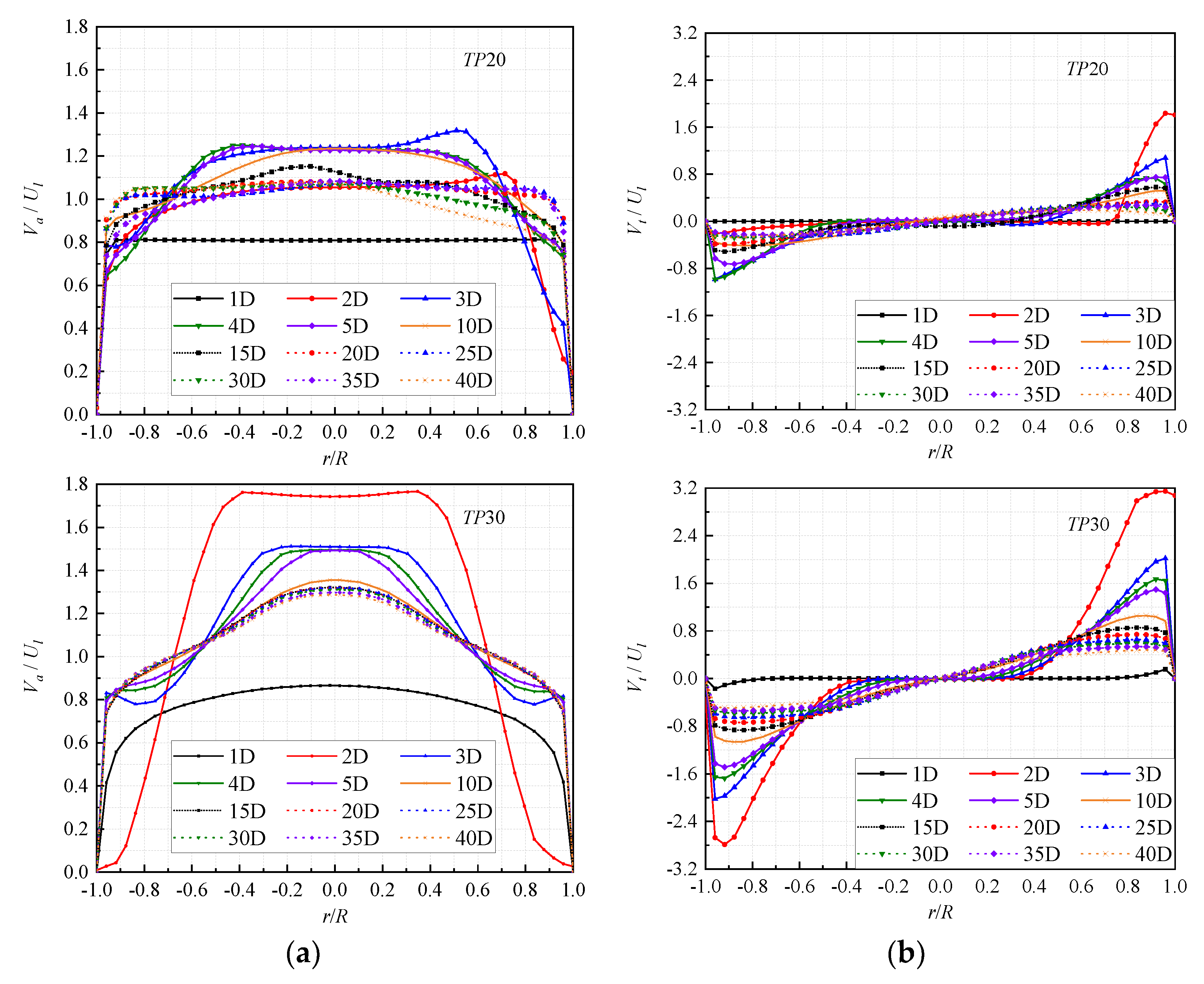
3.1.1. Flow Velocity Distribution

Figure 9 shows the comparison of dimensionless axial velocity (v_a/U_l) and tangential velocity (v_t/U_l) in different tangential proportion conditions at different observation planes along the flow direction, and U_l is the inlet velocity of STP. The axial and tangential velocities of each observation plane are time averaged, and the radial distance distribution of the pipe in the figure is a horizontal axis (r/R).

As shown in Figure 9a, the distribution of v_a/U_l of the swirling pipe is significantly different from that in the straight pipe. In the straight pipe, v_a/U_l presents a symmetric bullet-like distribution structure, while in the swirling pipe it presents an asymmetric periodic rotation distribution. Although v_a/U_l presents an asymmetrical distribution in TP10 and TP20, the distribution structure of TP10 and TP20 is generally similar to STP, while v_a/U_l presents a completely different degree of change in TP30. At the same time, in the swirling pipe, except for the section y = 1D, the v_a/U_l of other planes is higher than that of the straight pipe. The v_a/U${}_l$ of TP10 is not much different from STP, while the v_a/U${}_l$ of TP20 and TP30 are significantly higher than that of STP. Especially at y = 2D, the v_a/U${}_l$ of TP30 is about 1.7 times that of STP.

From 1D to 40D, the v_a/U${}_l$ of STP increases first and then decreases to a stable value with the observation plane away from the inlet. The variation trend of v_a/U${}_l$ of TP10 is similar to that of STP, and the difference is that the v_a/U${}_l$ of TP10 exhibits asymmetric distribution structure due to the effect of the tangential jet. At the same time, because the tangential jet accounts for part of the flow, the v_a/U${}_l$ of the swirling pipe at y = 1D is lower than that of the straight pipe, especially in TP20 and TP30. The asymmetrical distribution of TP20 is similar to that of TP10, but due to the increase in the proportion of tangential flow, the v_a/U${}_l$ of TP20 at the 2D to 5D section is higher than that of TP10, and then gradually decreases to a similar stable value. The v_a/U${}_l$ of TP30 presents a good periodic distribution. At y = 2D, due to the large tangential flow entering the pipe, the v_a/U${}_l$ immediately climbs to 2.2 times that of 1D, and then gradually decreases to a stable value which is higher than that of other cases.

In addition to the axial velocity, the tangential velocity also directly affects the flow structure in the pipe, and the magnitude of the tangential velocity affects the intensity of the swirling flow. As shown in Figure 9b, the dimensionless tangential velocity (v_t/U${}_l$) varies significantly from TP10 to TP30. The v_t/U${}_l$ of TP30 is the largest, TP20 is the second and TP10 is the smallest. At the same time, the v_t/U${}_l$ of STP is so small that it can be ignored when displayed on the same order of magnitude as the swirling pipe. The v_t/U${}_l$ of TP30 is about 1.7 times that of TP20 and more than 4 times that of TP10, indicating that the swirling intensity of TP30 should be significantly stronger than that of other cases.

From 1D to 40D, the distribution trend of v_t/U${}_l$ in each case is similar, and gradually decreases along the flow direction, which also indicates the attenuation of the corresponding swirling intensity. In addition, from 1D to 40D, v_t/U${}_l$ gradually decreases in the range of r/R = −1~−0.5 and 0.5~1, and in the range of r/R = −0.5~0.5, v_t/U${}_l$ gradually increases. This reflects the process of convergence and development of the tangential jet and the mainstream axial flow.

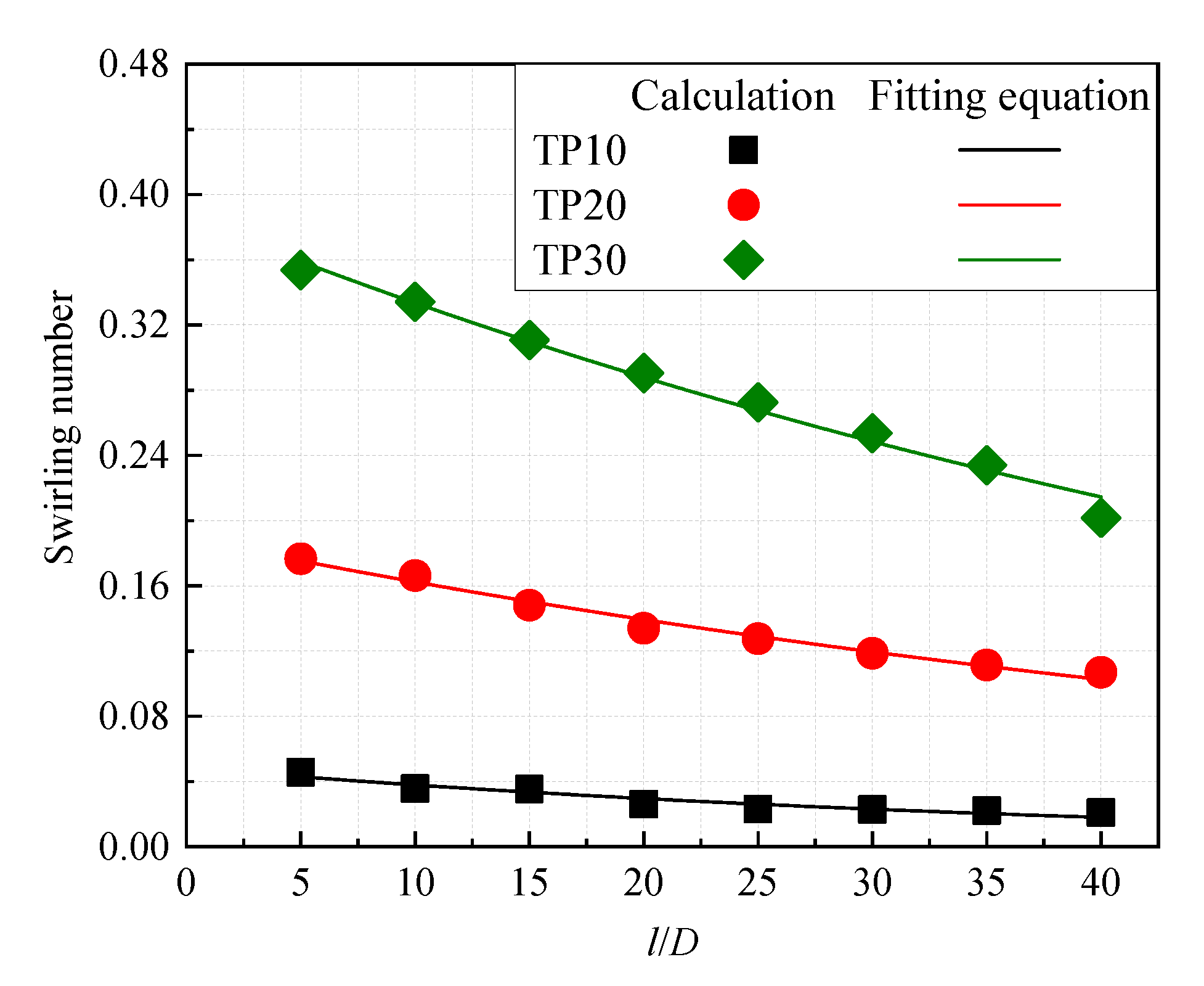
3.1.2. Swirling Intensity

The swirl number, which is the ratio of the hoop flux to the axial flux of the flow field [10,11,35], is a parameter to measure the strength of fluid rotation, and also is the most commonly used characterization parameter of swirling intensity, which is used to quantitatively analyze the rotation characteristics of the swirling pipe in this paper. The equation is expressed as:

$$S=\frac{1}{R}\times \frac{{\displaystyle \underset{0}{\overset{R}{\int }}{v}_A{v}_t{r}^{2}dr}}{{\displaystyle \underset{0}{\overset{R}{\int }}{v}_A^{2}rdr}}$$

(12)

where R is the radius; r is the radial distance; v_A and v_t are the axial and tangential velocities, respectively.

The tangential velocity of STP is too small to be ignored, and the swirling number of other cases is calculated by Equation (12), as shown in Figure 10. It can be seen from Figure 10 that the swirling number of each observation plane gradually decays along the flow direction and the swirling number of TP30 is the largest, which is about twice that of TP20 and 9 times that of TP10, respectively. However, it can also be seen that the decay rate of the swirling number varies from case to case. From 5D to 40D, the swirling number of TP30 is attenuated by 43.0%, TP20 and TP10 are attenuated by 39.5% and 54.1%, respectively, which shows that TP20 has a good swirling effect.

At present, the attenuation law of the swirling number has been clearly verified by Li and Tomita (1994) and Algifri et al. (1987), which conforms to the following exponential law.

$$S=S_0{e}^{cl/D}$$

(13)

where S₀ and c are constants, and the swirling number is fitted according to Equation (13). As shown in

Table 5. Equations of swirling number for different tangential proportions.

Case	TP10	TP20	TP30
Equation	$S=0.04856{\mathrm{e}}^{-0.02489l/D}$	$S=0.18928{\mathrm{e}}^{-0.01533l/D}$	$S=0.38631{\mathrm{e}}^{-0.01471l/D}$

, the fitting residual is in the order of 1× 10⁻⁵.

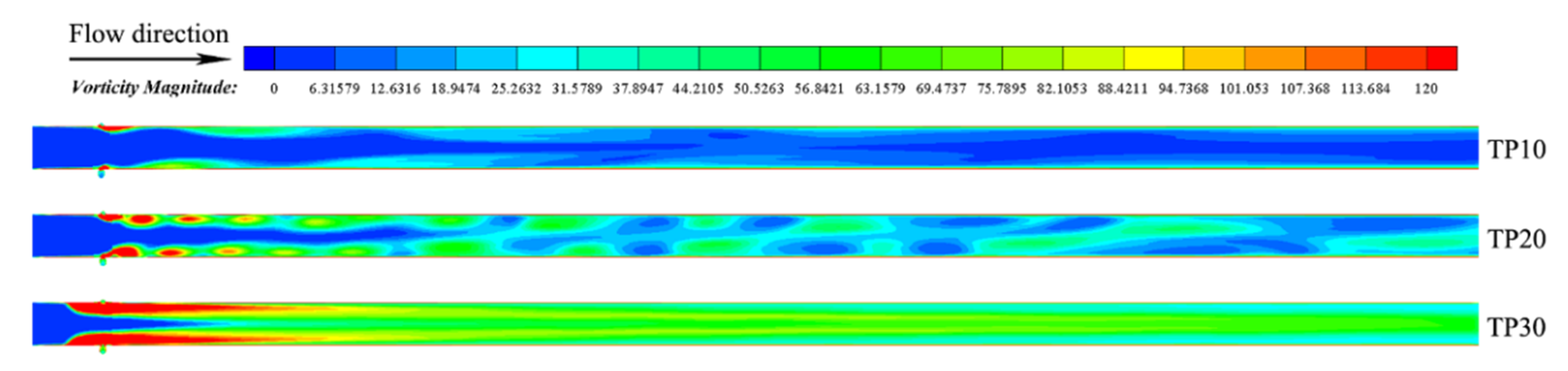
3.1.3. Vortex Structure

The vorticity is defined as the curl of the fluid velocity vector, which is usually used to measure the strength and direction of the vortex. In order to display the figure reasonably, the cloud chart of vorticity is placed horizontally in this paper. Figure 11 shows the vorticity cloud chart of the axis plane of the flow field to visually analyze the swirling intensity of each swirling pipe.

As shown in Figure 11, the vorticity distribution is similar. The vorticity value is low in the inlet region upstream of the tangential inlet and is the largest in the tangential inlet region, and then decreases gradually along the flow direction. In addition, it can be seen that the vorticity value in the near-wall region is significantly larger than the central region, especially at the inlet. Subsequently, as the fluid flows, the rotational flow in the near-wall region gradually merges with the internal axial flow, and the vorticity gap between the near-wall region and the central region decreases.

It can be seen that from TP10 to TP30, the vorticity intensity gradually increases, and the periodicity of the vorticity distribution is stronger. This is due to the increase in the swirling intensity caused by the increase in tangential velocity, namely, the increase in the proportion of tangential flow. Since the vorticity can only measure the intensity of the fluid vortex, the Q-criterion is introduced to extract the vortex core structure to further reflect the shape and position of the vortex. Q-criterion is the quadratic invariant of velocity gradient tensor, which is defined as:

$$Q=({\mathsf{\Omega }}_{ij}{\mathsf{\Omega }}_{ij}-S_{ij}{S}_{ij})/2$$

(14)

where Ω_ij and S_ij are symmetric tensor and antisymmetric tensor in velocity gradient tensor, respectively. The two tensors are defined as:

$$S_{ij}=(u_{ij}+u_{ji})/2$$

(15)

$${\mathsf{\Omega }}_{ij}=(u_{ij}-u_{ji})/2$$

(16)

Q represents the degree to which Ω_ijΩ_ij of the rotation rate is larger than S_ijS_ij. The Q-criterion well reflects a balance between deformation and rotation of fluid clusters in the flow field. At the position of Q > 0, the rotation rate Ω is dominant, that is, the vortex structure is dominant in this region. The vortex structures from TP10 to TP30 are extracted with the same Q value, and the pressure cloud chart is added on the iso-vortex surface, as shown in Figure 12.

It can be seen from Figure 12 that there is an obvious vortex core in the central region, indicating that the fluid has obvious rotational motion in this region. Three vortex cores occur at the three tangential entrances at the same time, and then grow with the rotation of the flow, and at the same time gradually break and merge into one vortex core with the attenuation of the swirling intensity.

From TP10 to TP30, the rotation angle of vortex core gradually decreases, and the vortex core of TP30 directly merges into a vortex core and grows downstream. This is because from TP10 to TP30, with the increase of the proportion of tangential flow, the tangential velocity of the flow field increases, and the axial stroke in the unit circumferential stroke decreases.

3.2. Load Particles

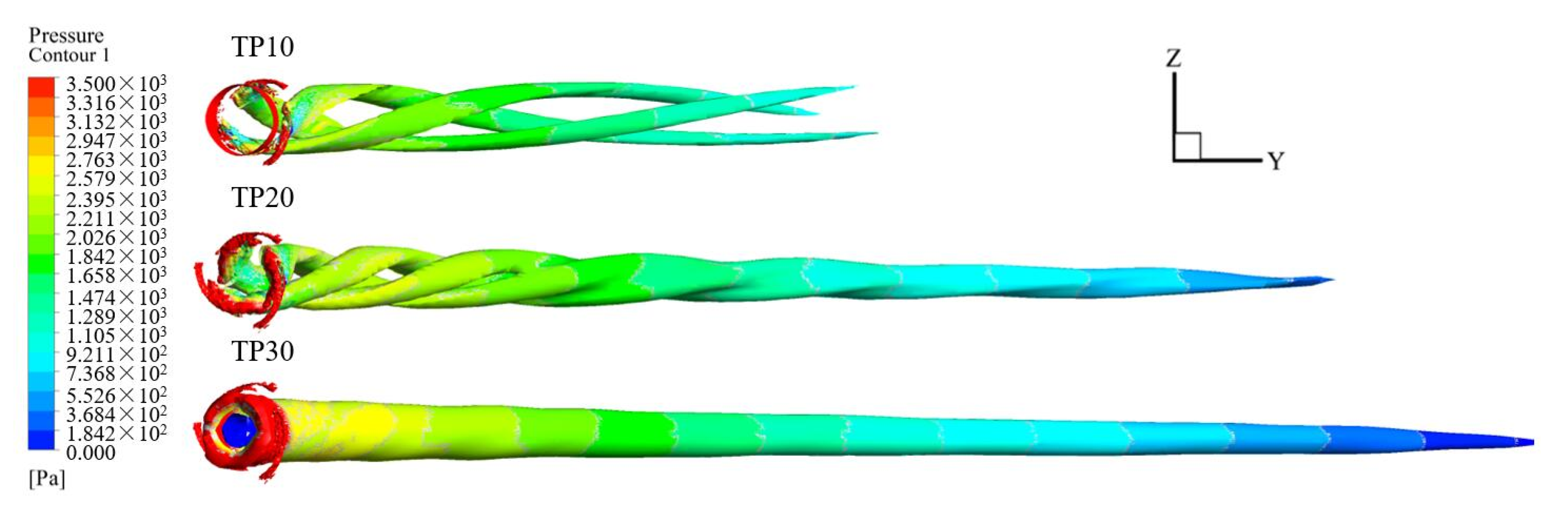
3.2.1. Pressure Distribution

The total pressure is the sum of the dynamic pressure and the static pressure of the flow field, which represents the total energy of the flow system. The total pressure drop is the change in the total pressure value of the two observation planes, which characterizes the degree of energy dissipation in the flow field. The total pressure value at each observation section is time-averaged, and the dimensionless processing is performed as follows:

$$P^{*}=\frac{P}{3{\rho }_l{U}_l^2}$$

(17)

where P^* is the dimensionless total pressure, P is the total pressure at each observation plane, ${\rho }_l$ is the density of seawater and U${}_l$ is the mainstream velocity without tangential flow.

Figure 13 shows the dimensionless total pressure P^* of four different tangential proportions. In general, the P^* value of each case shows a downward trend along the flow direction, and finally tends to be equal at the end of the flow. However, it can be clearly seen that at y = 2D, P^* of the swirling pipe has increased significantly, while P^* of the straight pipe curve remains smooth. This is because in the swirling pipe, the high-pressure tangential jet meets the main flow at y = 2D. In this area (y = 2D), the fluid medium increases instantly, and the pressure increases. From TP10 to TP30, the tangential proportion gradually increases, that is, the velocity of tangential jet flow gradually increases, and the influx of fluid medium gradually increases as the pressure increases, so the total pressure value at y = 2D gradually increases.

On the other hand, in the downstream region after y = 2D plane, the drop gradient of P* in each case is similar. From TP30 to TP10, the drop gradient of P* gradually decreases, which almost coincides with the drop curve of STP in TP10. This reflects that the swirling intensity of different tangential proportions is related to the loss of energy. TP30 has the highest swirling intensity but the highest energy loss, and TP10 is the opposite. Meanwhile, TP20 has higher swirling intensity and lower energy loss, which indicates that TP20 has better energy efficiency of rotation.

3.2.2. Particle Transport Status

When the calculation reaches the stable state, 20 particles are randomly selected to track the motion trace. In this way, we can visually analyze the particle-phase motion state of each tangential proportion case, as shown in Figure 14. In order to facilitate analysis, the flow process of each case is partitioned.

It can be clearly seen from Figure 14 that the particle motion trace in straight pipe is almost a straight line, while the particles in swirling pipes show periodic movement. In TP30, the particles first perform a short-term axial movement after formation. After entering the tangential jet area, the particles in the near-wall region rotate with the action of the tangential jet, and the particles in the central region maintain axial motion, that is, the particles are in a composite motion state. Then, the axial flow in the central region and the swirling flow in the near-wall region gradually merge, and all the particles in the pipe are in a rotating state. At the outlet, the swirl intensity decreases to a lower level, and the particles are in the state of a weak rotational motion. The flow process of TP20 is similar to that of TP30. This is because the swirl intensity of TP20 is lower than that of TP30, but the swirling decay rate of TP20 is also lower (Figure 10), so the distance of particle composite motion is similar. Because of the low tangential proportion of TP10, the swirling intensity is low, so the distance of the particle composite movement state is short.

In order to analyze the influence of the particle motion state on particle phase concentration distribution, the number concentration of particles C_N is defined as follows:

$$C_N=\frac{N_P}{A\times {10}^3}$$

(18)

where C_N is the particle number concentration, N_P is the time average number of all particles in 1D length and A is the cross-sectional area of the pipe.

It can be seen from Figure 15 that the particles at the inlet region are enriched due to the lower velocity, and the C_N gradually decreases until it tends to be stable. It can be seen that during the whole flow process, the C_N of the swirling pipe is higher than that of the straight pipe, which indicates that the swirling flow formed by the tangential jet has an enrichment effect on particles. From TP10 to TP30, the C_N gradually rises. Because with the increase of the swirling intensity, the axial movement distance in the unit circular movement period decreases (Figure 14), so the particle enrichment effect is more significant, that is, the particle-phase concentration increases more significantly.

Due to the different shapes of each component particle, the motion state in the swirling field is also different, which leads to the difference in the concentration distribution of each component particle with the same rated concentration. In order to analyze the concentration distribution law of each component particle in the swirling field, the relative fluctuation of the particle concentration C_f of each shape is analyzed, which is defined as follows:

$$C_f=\frac{N_{SP}}{0.25N_P}-1$$

(19)

where $C_f$ is the relative fluctuation of particle concentration of a certain shape, N_SP is the time average number of the particles in 1D length and N_P is the time average number of all particles in 1D length.

The $C_f$ is calculated by Equation (19), as shown in Figure 16. It can be seen that there are significant differences in the concentration of different components of particles in different cases. Firstly, the influence of swirling flow on $C_f$ is compared only from the perspective of different cases. In the straight pipe, although the concentration of each component particle is different, the difference and symbol of $C_f$ are similar throughout the flow process. This shows that the motion state of each component particle in straight pipe is relatively stable, which is consistent with the motion trace in Figure 14. In the swirling pipe, while the particle concentration of each component is different, the value of $C_f$ of each component particle fluctuates greatly, and the symbol changes quasi-periodically. From TP10 to TP30, with the gradual increase of the swirling intensity, the fluctuations of value and periodic changes of the symbol of $C_f$ become more and more obvious, which indicates that the steady motion state of the particles has been greatly changed.

Then, the particles of different components in different cases are analyzed. The concentration of spherical particles is significantly higher than that of non-spherical particles, which reflects the difference in the retention effect of particles of different components during the transportation process, that is, the difference in velocity of particles of different components. In the straight pipe, spherical particles have the largest $C_f$ and cylindrical particles have the smallest $C_f$, which indicates that the lifting speed of spherical particles is the slowest and the retention is the most, and the cylindrical particles are the opposite. The $C_f$ of the tetrahedral particles and the ellipsoidal particles are close, which indicates that their lifting rates are close, and their retention degrees are the same.

In the swirling pipe, the $C_f$ of spherical particles and cylindrical particles no longer maintain the maximum and minimum but reduces the difference with the tetrahedral particles and ellipsoidal particles, and there are periodic changes. That is to say, the $C_f$ values of the four kinds of particles are no longer significantly different, the overall lifting effect is better, and the mixing of each component particle is more uniform. This phenomenon is especially obvious in TP20, and the $C_f$ values of the four components are almost the same in the export area, which indicates that TP20 has a good transport state.

3.2.3. Drag Force and Kinetic Energy of Different Particles

In the process of hydraulic transportation, the flow structure of the particles is directly determined by the drag force on the particles. In order to further reveal the action mechanism of the swirling flow on the particles of each component, the dimensionless axial drag force (F_DA/F_G) and the dimensionless radial drag force (F_DR/F_G) of the particles during the entire flow process are analyzed, and the scatter diagram of drag force on all particles after stable flow is drawn, as shown in Figure 17.

It can be seen from Figure 17a that the F_DA/F_G of different components of particles is significantly different. The F_DA/F_G of cylindrical particles is the largest, which of spherical particles is the smallest, and the F_DA/F_G of ellipsoidal and tetrahedral particles is close. Then the F_DA/F_G of different components of particles tends to approach, and both decrease along the flow direction. In the straight pipe, the difference of F_DA/F_G between cylindrical particles and spherical particles is obvious, which leads to the difference of lifting velocity between cylindrical particles and spherical particles in the straight pipe, resulting in different retention effect and concentration distribution (Figure 16). Compared with the straight pipe case, the difference of F_DA/F_G between the swirling pipe cases is smaller. The difference of F_DA/F_G of each component in the initial stage (y = 0~10D) is reduced, and the F_DA/F_G of each component in the conveying section (y = 10~35D) is increased. From TP10 to TP30, with the increase of swirl intensity, the change trend of drag force increases gradually. As a result, the difference of lifting velocity of each component particles are reduced, and the retention of particles is similar. Therefore, the particles of each component are uniformly mixed and upgraded, and the overall lifting effect is better.

It can be seen from Figure 17b that the F_DR/F_G of the straight pipe is too small to be ignored, and there is a relatively high radial drag in the initial region of the swirling pipe. Along the flow direction, the F_DR/F_G of the swirling pipe gradually decreases with the attenuation of the swirl intensity, and the F_DR/F_G in the initial region increases gradually from TP10 to TP30. This shows that the swirling flow can disperse the particles in the initial stage and prevent the particles from silting in the pipeline. In addition, it can still be seen that cylindrical particles have the largest F_DR/F_G, spherical particles have the smallest F_DR/F_G and ellipsoidal particles have similar F_DR/F_G to tetrahedral particles, which is consistent with the distribution of F_DR/F_G.

4. Conclusions

In order to improve the efficiency and safety of vertical hydraulic transport systems for non-spherical particles, a new pipeline transport system with a tangential jet inlet is adopted in this study, and a modified non-spherical drag coefficient model is used to analyze the liquid-solid flow characteristics based on the CFD-DEM coupling method. The conclusions are as follows.

(1) The distribution of axial velocity presents a symmetrical bullet-like distribution structure in the straight pipe and presents an asymmetric periodic rotation distribution in the swirling pipe. The axial velocity and tangential velocity of the swirling pipe are significantly higher than that of the straight pipe, and this difference increases with the increase of the tangential flow proportion.

(2) The maximum vorticity appears in the tangential inlet region, and the vorticity in the near-wall region is significantly larger than that in the central region. With the increase of the tangential flow proportion, the swirling number and the vorticity intensity increases gradually, the helix angle of vortex core decreases gradually, and the breaking and merging of the vortex core occur more rapidly.

(3) The total pressure value of each case shows a downward trend along the flow direction. The descending gradient gradually increases with the increase of the tangential flow proportion, reflecting the difference of energy efficiency of different tangential flow proportions.

(4) The particle number concentration of the swirling pipe is higher than that of the straight pipe, and the particle number concentration increases with the increase of tangential flow proportion. Meanwhile, the concentration difference of the particles of different components is reduced by the effect of the swirling flow in the swirling pipe, and the particles of each component are uniformly mixed and lifted.

(5) The axial drag force of different components of particles differs greatly in the straight pipe, the axial drag force of cylindrical particles is the largest, which of spherical particles is the smallest, and the axial drag force of ellipsoidal and tetrahedral particles is close. Moreover, the difference of axial drag force in the swirling pipe is reduced by the effect of the swirling flow. The radial drag force is larger in the initial section of the swirling pipe, and then gradually decreases along the flow direction.

References

1. Tang, D.S.; Yang, N.; Jin, X. Hydraulic lifting technique with vertical pipe for deep-sea coarse mineral particles. Min. Metall. Eng. 2013, 33, 1–8. [Google Scholar]
2. Bai, X.N.; Gen, H.S.; Zhang, D.F.; Qin, H.B. Advances and applications of solid-liquid two-phase flow in pipeline hydrotransport. J. Hydrodyn. 2001, 16, 303–311. [Google Scholar]
3. Hein, J. Cobalt-rich ferromanganese crusts: Global distribution, composition, origin and research activities. Int. Seabed Auth. 2003, 5, 36–89. [Google Scholar]
4. Baker, E. Quantifying the global distribution of hydrothermal venting. In The 2nd Seabed Scientific Forum-Continental Margin and Ocean Ridge; SOA: Bhubaneswar, India, 2007. [Google Scholar]
5. Durand, R.; Condolios, E. The Hydraulic Transportation of Coal and Solid Materials in Pipes; Collage of National Coal Board: London, UK, 1952; pp. 39–52. [Google Scholar]
6. Xu, Z.L. A new model for interpretating the velocity distribution of a heterogeneous flow in horizontal pipe. Hydraul. Coal Min. Pipeline Transp. 1998, 4, 34–40. [Google Scholar]
7. Asakura, K.; Asari, T.; Nakajima, I. Simulation of solid—liquid flows in a vertical pipe by a collision model. Powder Technol. 1997, 94, 201–206. [Google Scholar] [CrossRef]
8. Xia, J.X.; Ni, J.R.; Mendoza, C. Hydraulic Lifting of Manganese Nodules Through a Riser. J. Offshore Mech. Arct. Eng. 2004, 126, 72–77. [Google Scholar] [CrossRef]
9. Pinto, T.S.; Júnior, D.M.; Slatter, P.; Filho, L.D.S.L. Modelling the critical velocity for heterogeneous flow of mineral slurries. Int. J. Multiph. Flow 2014, 65, 31–37. [Google Scholar] [CrossRef]
10. Li, H.; Tomita, Y. Characteristics of Swirling Flow in a Circular Pipe. J. Fluids Eng. 1994, 116, 370–373. [Google Scholar] [CrossRef]
11. Li, H.; Tomita, Y. An Experimental Study of Swirling Flow Pneumatic Conveying System in a Horizontal Pipeline. J. Fluids Eng. 1996, 118, 526–530. [Google Scholar] [CrossRef]
12. Fokeer, S.; Lowndes, I.; Kingman, S. An experimental investigation of pneumatic swirl flow induced by a three lobed helical pipe. Int. J. Heat Fluid Flow 2009, 30, 369–379. [Google Scholar] [CrossRef]
13. Fokeer, S.; Lowndes, I.; Hargreaves, D. Numerical modelling of swirl flow induced by a three-lobed helical pipe. Chem. Eng. Process. Process. Intensif. 2010, 49, 536–546. [Google Scholar] [CrossRef]
14. Zhou, J.-W.; Du, C.-L.; Liu, S.-Y.; Liu, Y. Comparison of three types of swirling generators in coarse particle pneumatic conveying using CFD-DEM simulation. Powder Technol. 2016, 301, 1309–1320. [Google Scholar] [CrossRef]
15. Rinoshika, A. Self-excited pneumatic conveying of granular particles in various horizontal curved 90° bends. Exp. Therm. Fluid Sci. 2015, 63, 9–19. [Google Scholar] [CrossRef]
16. Yan, F.; Luo, C.; Zhu, R.; Wang, Z. Experimental and numerical study of a horizontal-vertical gas-solid two-phase system with self-excited oscillatory flow. Adv. Powder Technol. 2019, 30, 843–853. [Google Scholar] [CrossRef]
17. Yin, J.; Chen, Q.Y.; Zhu, R.; Tang, W.X.; Su, S.J.; Yan, F.; Wang, L.H. Enhancement of liquid-solid two-phase flow through a vertical swirling pipe. J. Appl. Fluids 2020, 13, 1501–1513. [Google Scholar]
18. Zhong, W.-Q.; Zhang, Y.; Jin, B.-S.; Zhang, M.-Y. Discrete Element Method Simulation of Cylinder-Shaped Particle Flow in a Gas-Solid Fluidized Bed. Chem. Eng. Technol. 2009, 32, 386–391. [Google Scholar] [CrossRef]
19. Tran-Cong, S.; Gay, M.; E Michaelides, E. Drag coefficients of irregularly shaped particles. Powder Technol. 2004, 139, 21–32. [Google Scholar] [CrossRef]
20. Ren, B.; Zhong, W.Q.; Jiang, X.F.; Jin, B.S.; Yuan, Z.L. Numerical simulation of spouting of cylindroid particles in a spouted bed. Can. J. Chem. Eng. 2014, 92, 928–934. [Google Scholar] [CrossRef]
21. Molaei, E.A.; Yu, A.; Zhou, Z. CFD-DEM modelling of mixing and segregation of binary mixtures of ellipsoidal particles in liquid fluidizations. J. Hydrodyn. 2019, 31, 1190–1203. [Google Scholar] [CrossRef]
22. Hölzer, A.; Sommerfeld, M. New simple correlation formula for the drag coefficient of non-spherical particles. Powder Technol. 2008, 184, 361–365. [Google Scholar] [CrossRef]
23. Shih, T.-H.; Liou, W.W.; Shabbir, A.; Yang, Z.; Zhu, J. A new k-ϵ eddy viscosity model for high reynolds number turbulent flows. Comput. Fluids 1995, 24, 227–238. [Google Scholar] [CrossRef]
24. Ghaya, H.; Guizani, R.; Mhiri, H.; Bournot, P.; Iusti, T.D.C.-G. CFD Study of the Effect of Geometrical Shape of Separation Blades on the Rotor Performance of an Annular Centrifugal Extractor (ACE). J. Appl. Fluid Mech. 2019, 12, 1189–1202. [Google Scholar] [CrossRef]
25. Zhou, F.; Hu, S.; Liu, Y.; Liu, C.; Xia, T. CFD–DEM simulation of the pneumatic conveying of fine particles through a horizontal slit. Particuology 2014, 16, 196–205. [Google Scholar] [CrossRef]
26. Di Felice, R. The voidage function for fluid-particle interaction systems. Int. J. Multiph. Flow 1994, 20, 153–159. [Google Scholar] [CrossRef]
27. Bagheri, G.; Bonadonna, C. On the drag of freely falling non-spherical particles. Powder Technol. 2016, 301, 526–544. [Google Scholar] [CrossRef] [Green Version]
28. Hilton, J.; Mason, L.; Cleary, P. Dynamics of gas–solid fluidised beds with non-spherical particle geometry. Chem. Eng. Sci. 2010, 65, 1584–1596. [Google Scholar] [CrossRef]
29. Zhou, Z.; Pinson, D.; Zou, R.; Yu, A. Discrete particle simulation of gas fluidization of ellipsoidal particles. Chem. Eng. Sci. 2011, 66, 6128–6145. [Google Scholar] [CrossRef]
30. Rong, L.; Zhou, Z.; Yu, A. Lattice–Boltzmann simulation of fluid flow through packed beds of uniform ellipsoids. Powder Technol. 2015, 285, 146–156. [Google Scholar] [CrossRef]
31. Tsuji, T.; Yabumoto, K.; Tanaka, T. Spontaneous structures in three-dimensional bubbling gas-fluidized bed by parallel DEM–CFD coupling simulation. Powder Technol. 2008, 184, 132–140. [Google Scholar] [CrossRef]
32. Karimi, H.; Dehkordi, A.M. Prediction of equilibrium mixing state in binary particle spouted beds: Effects of solids density and diameter differences, gas velocity, and bed aspect ratio. Adv. Powder Technol. 2015, 26, 1371–1382. [Google Scholar] [CrossRef]
33. Xiong, C.Q.; Zhang, M.Y.; Fan, Q.Y. Numerical simulation of external flow field around low drag car and its error analysis. Automot. Eng. 2012, 34, 36–45. [Google Scholar]
34. Schlichting, H. Boundary Layer Theory, 7th ed.; Springer: Berlin/Heidelberg, Germany, 1979. [Google Scholar]
35. Klancisar, M.; Schloen, T.; Hribersek, M.; Samec, N. Analysis of the Effect of the Swirl Flow Intensity on Combustion Characteristics in Liquid Fuel Powered Confined Swirling Flames. J. Appl. Fluid Mech. 2016, 9, 2359–2367. [Google Scholar] [CrossRef]
Figure 1. Schematic diagram for pipe with tangential jet inlet: (a) spatial structure of the pipeline (b) plane distribution of tangential inlet.
Jmse 09 01091 g001
Figure 2. Schematic diagram of the conveying process of swirling pipe.
Jmse 09 01091 g002
Figure 3. Fluid domain meshing of swirling pipe.
Jmse 09 01091 g003
Figure 4. Maximum axial velocity at 5D position for different grid sizes and time steps.
Jmse 09 01091 g004
Figure 5. The accumulation of bed and the spherical filling of cylinder particles.
Jmse 09 01091 g005
Figure 6. Comparisons of particle patterns simulated by Sphere Model with Ren’s experiments and simulation.
Jmse 09 01091 g006
Figure 7. Comparisons of particle patterns simulated by non-sphere model with Ren’s experiments and simulation.
Jmse 09 01091 g007
Figure 8. Comparisons of simulated pressure drop with Ren’s experiments and simulation.
Jmse 09 01091 g008
Figure 9. Dimensionless velocity distribution: (a) dimensionless axial velocity (va/U l ); (b) dimensionless tangential velocity (vt/U l ).
Jmse 09 01091 g009aJmse 09 01091 g009b
Figure 10. Swirling number for different swirling pipes.
Jmse 09 01091 g010
Figure 11. Schemes follow the same formatting.
Jmse 09 01091 g011
Figure 12. Vortex structure for different swirling pipes based on iso-vortex surface.
Jmse 09 01091 g012
Figure 13. The dimensionless total pressure for different swirling pipes.
Jmse 09 01091 g013
Figure 14. The particle-phase motion state for different swirling pipes.
Jmse 09 01091 g014
Figure 15. The distribution of particle number concentration for different swirling pipes.
Jmse 09 01091 g015
Figure 16. The C f distribution of different components particles in different cases.
Jmse 09 01091 g016
Figure 17. Dimensionless drag force distribution: (a) FDA/FG; (b) FDR/FG.
Jmse 09 01091 g017