Article

Buoyancy Regulation Strategy for Underwater Profiler Based on Adaptive Genetic Algorithm

1
The State Key Laboratory of Fluid Power and Mechatronic Systems, Zhejiang University, Hangzhou 310027, China
2
Ningbo Research Institute, Zhejiang University, Hangzhou 315000, China
*
Author to whom correspondence should be addressed.
J. Mar. Sci. Eng. 2021, 9(1), 53; https://doi.org/10.3390/jmse9010053
Submission received: 1 December 2020 / Revised: 28 December 2020 / Accepted: 4 January 2021 / Published: 6 January 2021
(This article belongs to the Section Ocean Engineering)

Abstract

:
Considering the energy limitations of underwater vehicles, a strategy for energy saving is proposed. In the proposed buoyancy regulation strategy, oil of the buoyancy regulation system is pumped out several times at different depths instead of all at once. A balance between energy and time is achieved by assigning suitable weights, and the optimised depth which can be obtained from the pressure sensor is used as the judgement threshold based on the adaptive genetic algorithm. Through the numerical simulation using sea trial data, the influence of weight selection on energy and time is explored, and the frequency of oil draining for the vehicle to ascend is optimised. Simulation results show that the proposed buoyancy regulation strategy can save energy effectively when the frequency of oil draining is 4 times within depths of 0–500 m. Finally, trials were performed in Qiandao Lake and verify the contradictory relationship between energy and time.

1. Introduction

There are abundant marine resources on the Earth [1,2]. With the development of underwater technology, autonomous underwater vehicles [3], gliders [4,5], and buoys [6] have been developed for ocean observation. Energy is a crucial matter in the design process of underwater vehicles. Most underwater vehicles use lithium batteries, which have a high energy density, as an energy source [7,8]. More importantly, some underwater vehicles, such as underwater gliders, use lithium batteries as weights for attitude adjustments [9] to utilise the weight and space of the battery.
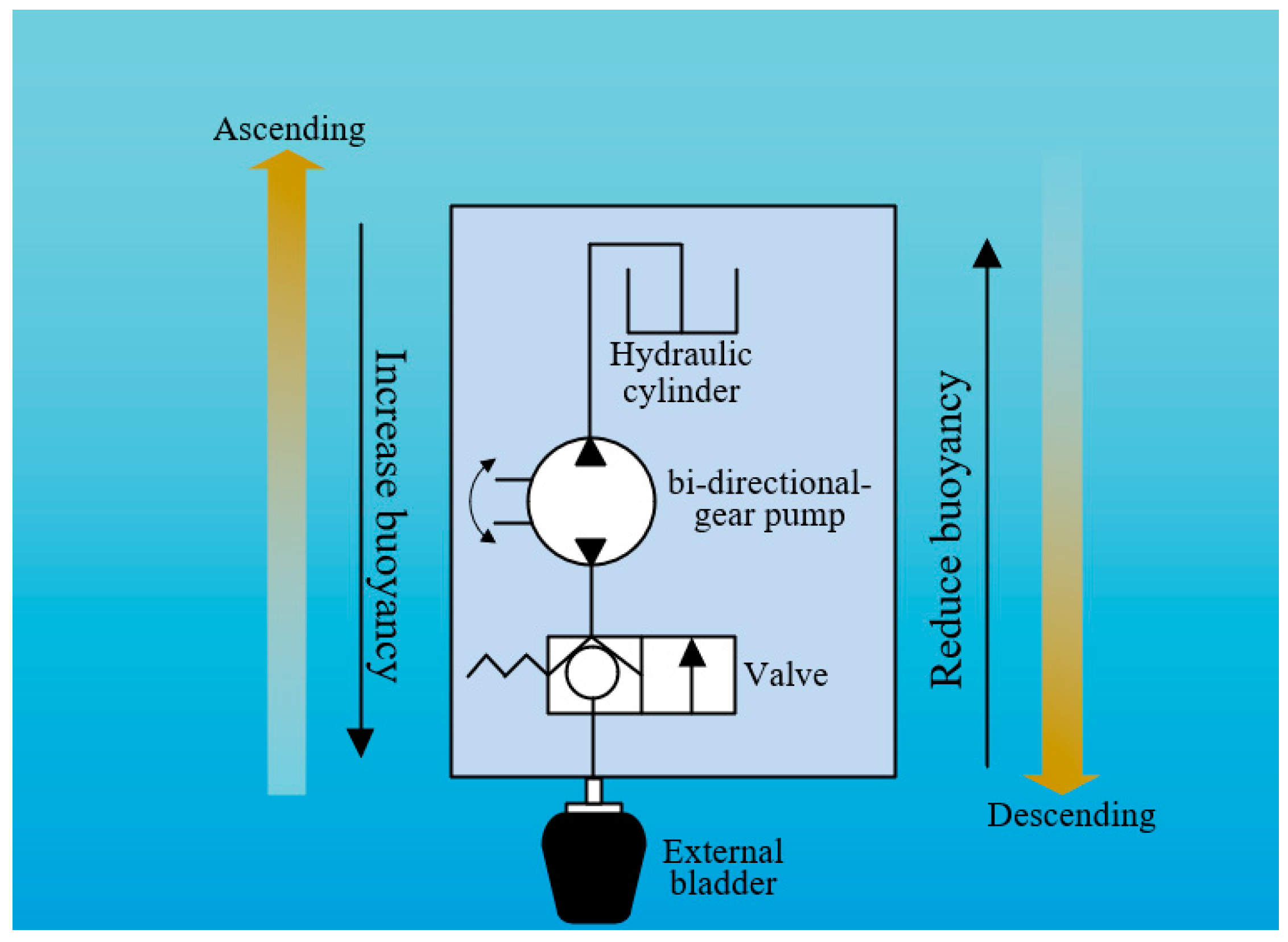
In general, underwater gliders and buoys are equipped with a buoyancy regulation system. Some buoyancy regulation systems increase their weight by pumping seawater into the body [10], and some increase their volume by pumping oil from an inner cylinder to an external bladder [11]. The two methods have one thing in common—both require a motor to drive the pump, and the energy required for this motor accounts for most of the overall energy consumption. Yazji et al. adjusted the volume of the vehicle by utilising electrolysis and reverse electrolysis of polymer electrolyte membrane fuel cell [12]. Um et al. changed the overall volume of the buoyancy regulation system by electrolysing water and then inflating an artificial bladder with the generated gas to increase buoyancy [13]. Although this method of changing the volume of gas is effective in a diving environment, depth control is difficult once the vehicle reaches the deep-water area because of the greater compressibility of the air. Therefore, the method of changing the volume by using hydraulic oil has been widely used.
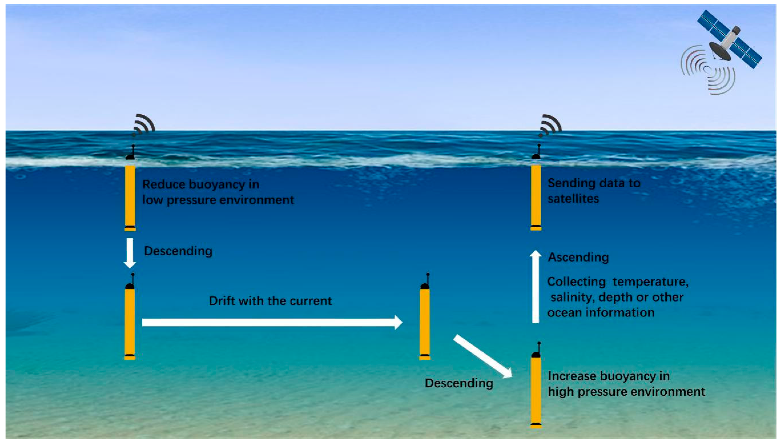
Figure 1 shows the typical working process of an underwater profiler. When the profiler prepares to descend, it pumps the oil from its outer oil bladder into its inner cylinder. When the profiler prepares to ascend, the reverse process is performed to increase the buoyancy. Generally, this process is performed all at once. As the depth increases, the power consumption of the motor of the buoyancy regulation system becomes larger [14]. Some researchers have explored buoyancy regulation strategies to save the energy of the profiler during the working process. Petzrick et al. [15] proposed pumping oil in small increments and maintaining the total ascent time within 20 h. Mu et al. [16] proposed an overall energy model for the floating process based on the multiple quantitative regulation strategy; through numerical calculation, they concluded that the system power consumption is the lowest when the buoyancy regulation system of a 4000-m-level submersible is adjusted 16 times during the floating process. Liu et al. [17] proposed a ‘stage quantitative oil draining control mode’, and the system parameters, including oil discharge resolution, judgement threshold of the floating speed, and frequency of oil draining, were optimised. These strategies and methods are instructive. It is necessary to establish accurate kinematic models and select appropriate judgement thresholds, especially considering the interference of ocean currents. In addition, it is meaningful to explore the contradictory relationship between energy and time during ascent for the development of appropriate mission assignments.
In this article, we propose a buoyancy regulation strategy with depth as the judgement threshold. Our strategy is based on the adaptive genetic algorithm (AGA) which is validated using a hybrid underwater profiler (HUP) [18] named Zhejiang University HUP (ZJU–HUP) in Qiandao Lake, China. The remainder of this article is organised as follows. Section 2 presents the principle of a buoyancy regulation system and the ascending kinematic model. Section 3 presents the operation process of the AGA. Section 4 presents the results of numerical simulations within a depth of 0–500 m using sea trial data obtained in July 2017. Finally, Section 5 presents the lake trial and the corresponding results.

2. Buoyancy Regulation System and Kinematic Model

2.1. Buoyancy Regulation System

The HUP designed by Zhejiang University is a buoyancy-driven vehicle that can realise small-scale ocean observations based on the station-keeping method [18]. It uses a bi-directional gear pump to pump oil—oil is pumped from the internal hydraulic cylinder to the external bladder to increase buoyancy and conversely, from the external bladder to the internal hydraulic cylinder to decrease buoyancy. The main specifications of the ZJU–HUP are listed in Table 1.
As shown in Figure 2, when the HUP starts to dive into the deep-water, the motor is turned on clockwise to drive the bi-directional-gear pump to let the oil flow from the hydraulic cylinder to the external bladder through the check valve. Note that the solenoid valve of the system is in the position of the one-way valve when the solenoid valve is not energised. Considerable electrical energy can be saved as there is no need to turn on the solenoid valve in the diving process. Meanwhile, the equipment inside the cavity is safer because the check valve prevents the backflow of the oil in the external bladder despite the high pressure on the external bladder in the deep-water region. When the HUP prepares to ascend to the water surface, the solenoid valve is turned on to let the oil in the internal cylinder flow to the external bladder to increase buoyancy.
Since the ocean density varies with depth, the volume of the external bladder of the profiler is suitably changed for the vessel to ascend or descend. When the profiler stays in a static state at a depth h x , a balance is attained between gravity and buoyancy:
ρ h x g V h x = m g
While the profiler moves to another depth h y , this balance is achieved in the same manner:
ρ h y g V h y = m g
where ρ h x and ρ h y are the densities of the seawater at depth h x and h y . Further, V h x and V h y are the drained water volume of the underwater vehicle at the corresponding depth. The difference in the volume of the external bladder that is to be achieved from depth h x to depth h y can be deduced as follows:
Δ V h x h y = | V h x V h y | = | m ρ h x m ρ h y |
To obtain the relationship between the motor power, speed of oil discharge, and depth, an experiment was performed based on the schematic diagram shown in Figure 3. In the experiment, a relief valve was used to simulate the external pressure acting on the pump. First, the relief valve was set at different pressures (from 0 MPa to 5 MPa), and then, the motor was turned on to pump the oil from the hydraulic cylinder to the external container. The time taken for oil discharge and the capacity of the external container were recorded to calculate the oil discharge speed. A galvanometer based on the Hall principle was used to measure the current of the motor. Then, the relations between motor power, speed of oil discharge and depth were obtained indirectly.
The experimental results are shown in Figure 4. The variation of motor power with depth can be described by a first-order polynomial fitting:
p h = p 1 h + p 2
where the fitted coefficients p 1 and p 2 are 0.032 and 19, respectively. The variation in the oil discharge speed with depth can be described by a third-order polynomial fitting:
V o = q 1 h 3 + q 2 h 2 + q 3 h + q 4
where the fitted coefficients q 1 , q 2 , q 3 and q 4 are 1.2 × 10 7 , 1.6 × 10 4 , 0.31 and 190 , respectively. The root mean squared error (RMSE) of the third-order polynomial fitting is 1.7 which means that the error is small and can be accepted.

2.2. Kinematic Model

During ascent, the HUP is subjected to gravity, drag force, and buoyancy. The drag force changes with the speed of the HUP as follows:
F f = 1 2 C v 2 S ρ
where C represents the resistance coefficient; v , is the speed of the HUP; S , the cross section in the radial direction of the aluminium alloy cavity; and ρ , the density of the water outside the HUP.
During ascent, the speed of the HUP changes as it is accelerated. Hence, the ascent is divided into small intervals for computational convenience. A small interval can be seen as a model of motion with constant acceleration in a sufficiently small time. The final speed of the first interval is calculated and used as the initial velocity for the next interval. Finally, the velocity distribution can be obtained through iterations. Therefore, the kinematic equation of one small interval is set up as follows:
m a = ρ g ( V + V out ) F f m g
where V o u t represents the volume of the external bladder, and V represents the volume of the HUP, excluding the external bladder.
According to the integral expression of acceleration:
a = d v d t
The speed of the HUP in the small interval during ascent is shown as follows:
v = a 1 a 2 tan h ( ( t 2 m + C 1 ) a 1 a 2 )
a 1 = 2 ρ g ( V + V out   ) 2 m g
a 2 = C · S
where C 1 represents the integral constant.
The integral expression of velocity is as follows:
v = d h d t
The movement equation of the displacement and time is established by substituting Equation (9) into Equation (12):
h = t · a 1 a 2 2 · m · log ( tan h ( a 1 a 2 · ( C 1 + t 2 m ) ) ) + 1 a 2 + C 2
where C 2 represents the integral constant. Using Equation (9) and Equation (13), the velocity and displacement of each subinterval are calculated and then the total displacement is obtained by summing up the displacements of all subintervals. The time of motion in the whole interval is the product of the number of subintervals and the step length.

3. Buoyancy Regulation Strategy

Based on the kinematics model established in Section 2, the optimal depth at which the oil is pumped needs to be solved. Since the kinematics model is nonlinear, it is difficult to use conventional methods. Currently, intelligent optimisation algorithms are widely used. Among them, the AGA is an intelligent optimisation method in which the probability of crossover and mutation changes with the value of the objective function; AGA can effectively prevent the search process from converging to the local optimum value. The AGA was applied to a variety of problems such as job-shop problems [19], optical metasurface design [20], and sensor acquisition frequency adjustment [21], and satisfactory optimisation results were obtained. To optimise the depth accurately and to prevent convergence to the local optimal value, the AGA was applied to the buoyancy regulation strategy.

3.1. Optimisation Principle and Process

In the AGA, the roulette method is used to select better individuals to prevent the loss of individuals with excellent genes. Gene recombination and mutation are important means of biological evolution. Similarly, two-parent individuals exchange partial structures to generate new individuals to improve the global search ability of the AGA. The individuals in the population can be mutated by changing the value at a certain gene position. Mutation may have two effects: one is to improve the local search ability of the AGA, and another is to maintain population diversity.
In the population of a certain generation, different individuals have different fitness values. A high fitness value indicates a better individual, and such an individual should be retained. So this individual should have a small crossover probability and mutation probability. Generally, the difference between the maximum fitness value and the average fitness value in a generation is defined as F d i f f for convenience. This value indicates the degree of convergence of the population. When the algorithm gradually converges, it may jump into the local optimal solution as F d i f f decreases gradually. In this situation, the crossover probability and the mutation probability should be increased to enable the system to jump out of the local optimal solution. On the other hand, in the population of a certain generation, excellent individuals should have small crossover probability and mutation probability, and poor individuals should have large crossover probability and mutation probability to accelerate the elimination process. Therefore, the crossover probability P c and mutation probability P m [22] are expressed as follows:
P c = { k 1 · f m a x f F d i f f , f f ˉ k 3     , f < f ˉ
P m = { k 2 · f m a x f F d i f f , f f ˉ k 4   , f < f ˉ
where f ¯ represents the average fitness value of the population; f m a x is the maximum fitness value of the population; f and f are the fitness value; k 1 , k 2 , k 3 , k 4 1.0 .

3.2. Construction of the Fitness Function

The fitness function is used to describe the adaptability of each individual in the environment, and it determines whether an individual can be retained. Individuals with high fitness values are more likely to be inherited to the next generation. For the buoyancy regulation strategy described herein, the minimum value of the fitness function should be calculated. This function has two parts, namely, energy and time. It can be expressed as follows:
f ( x ) = C m a x ( ω E · ( i = 1 k ( P h 1 · t o i ) ) + ω T · ( i = 1 k ( t i + t o i ) ) )
where C m a x is a positive number used to make the fitness function positive. ω E is the weight of energy and varies from 0 to 1. It represents the proportion of motor energy consumed of the buoyancy regulation device. ω T is the weight of time representing the overall time of the floating movement. The sum of ω E and ω T is 1. Furthermore, k is the frequency of oil drainage. P h i is the power consumption of the motor when pumping oil at depth h i , and t o i is the corresponding time. The floating time between two adjacent depth values is represented by t i , and it can be obtained by multiplying the number of subintervals by the step size.

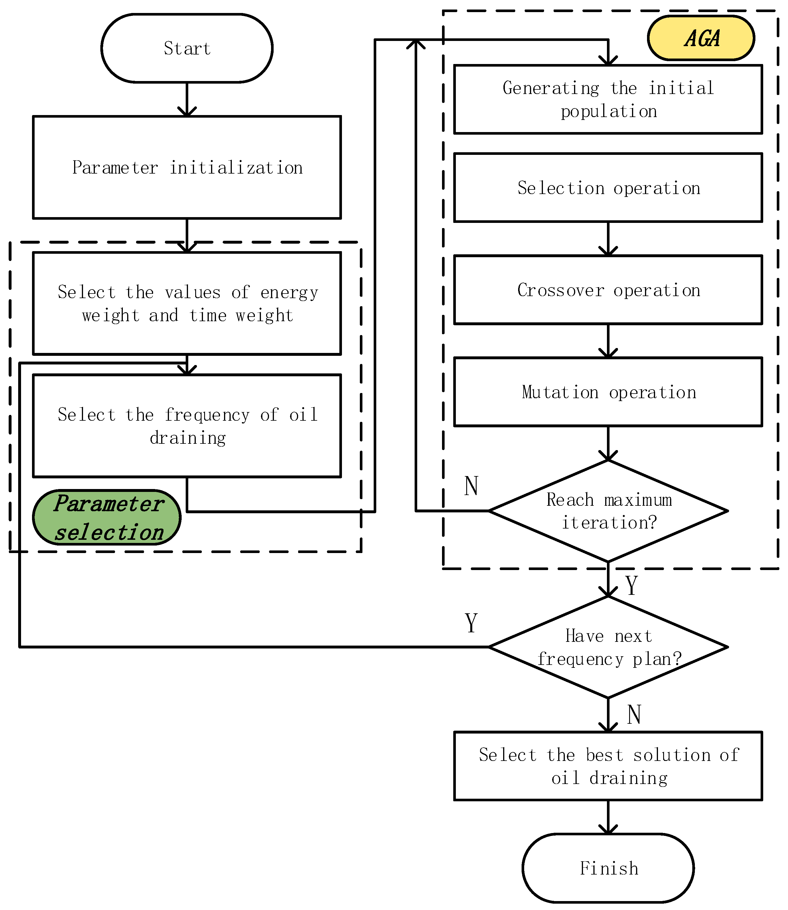
3.3. Adaptive Genetic Algorithm Process

The application of the AGA for the buoyancy regulation strategy involves the following steps and the corresponding flowchart is shown in Figure 5.
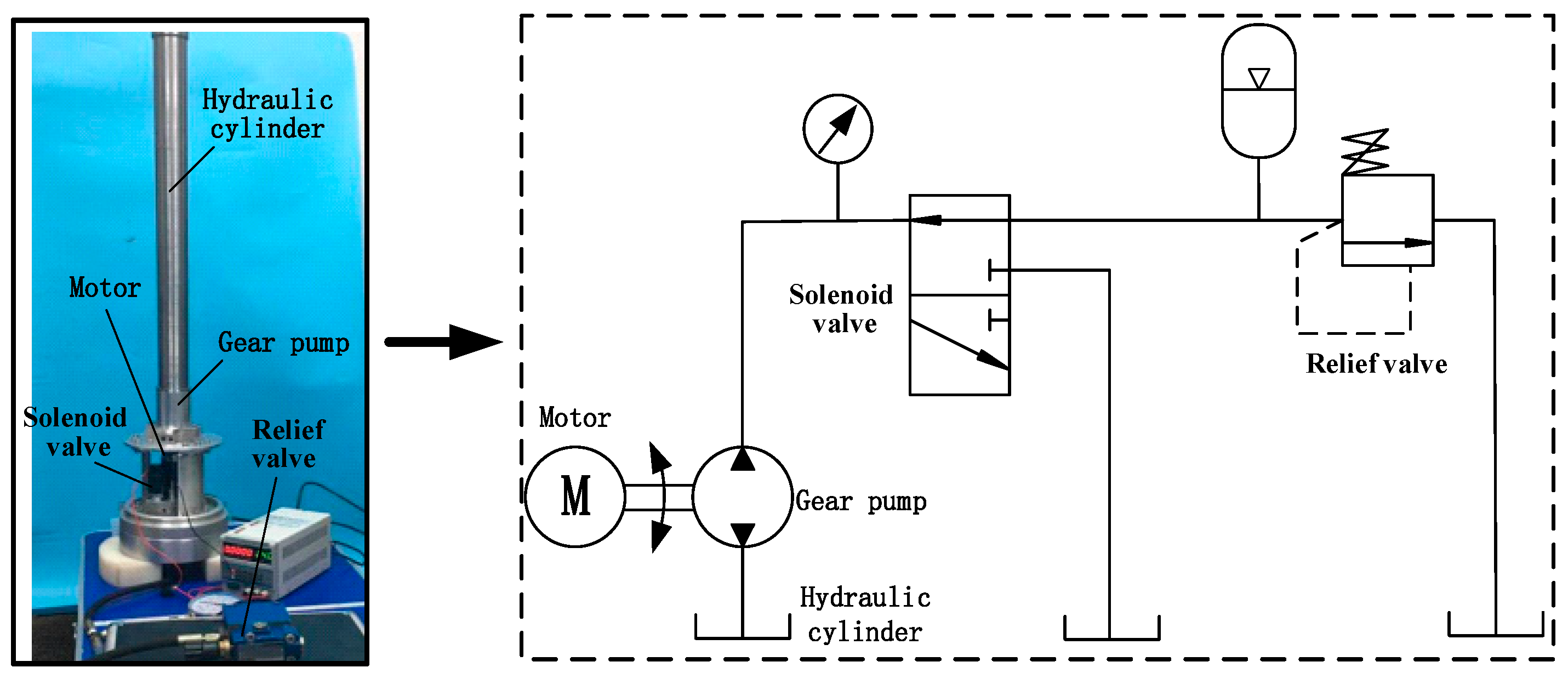
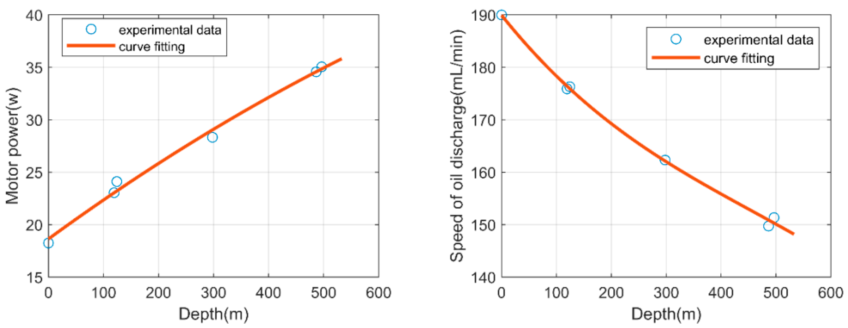
  • Step 1: Parameter initialisation. First, perform experiments on the buoyancy regulation system to obtain the relationship between the motor power and depth and the relationship between the oil draining rate and depth of the pump. Then, collect the temperature, salinity, and depth information when the profiler moves from the sea surface to the target depth to fit the relationship between the density and depth according to the EOS-80 equation [23].
  • Step 2: Select the values of power, weight and time weight. Based on the task requirements, if the requirements for low energy consumption are stringent and the time to perform the detection task is relatively sufficient, then a larger ω E is selected; if less time is available to perform the detection task, a larger ω T , that is, a smaller ω E is selected.
  • Step 3: Select the oil draining frequency. Different frequency values should be set in the AGA to compare energy and time at different oil draining frequencies.
  • Step 4: Generate the initial population. In the AGA, randomly generated depth is used as individuals. For frequency k , generate ( k 1 ) individuals randomly, that is, ( k 1 ) depth values, to generate a population consisting of ( k 1 ) depth values. The reason for setting the number of individuals in the population as 1 less than the frequency of oil draining is that the first depth value is fixed.
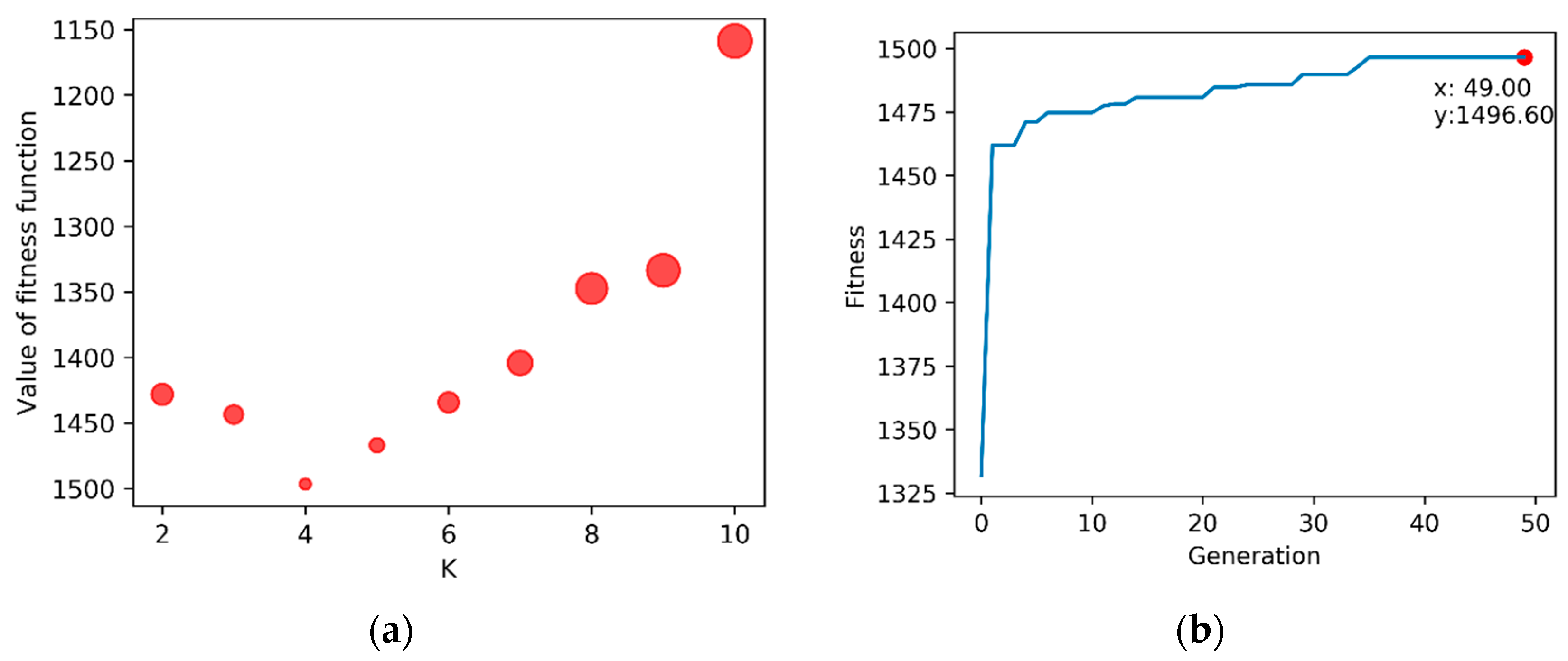
  • Step 5: Execute the AGA. A new population is obtained through three operations: selection operation, crossover operation, and mutation operation. The number of population is set to 10, and the number of generation is set to 50. The value of k 1 and k 3 is 1. The value of k 2 and k 4 is 0.1.
  • Step 6: Determine whether the maximum number of iterations is reached. The number of iterations should be sufficiently large to allow results to converge.
  • Step 7: When a plan is completed, record the optimal energy and time. Change the frequency of oil draining until all the steps are executed. Finally, the frequency of oil draining corresponding to the smallest fitness value can be used as the execution solution.

4. Numerical Simulations

4.1. Discussion on Weights of Time and Power

In general, underwater gliders or profilers pump all oil to their external bladder at once to increase buoyancy. This means that the weight of energy is 1, and that of time weight is 0. In July 2017, a ZJU-HUP profile measurement experiment was conducted in the South China Sea to verify its performance. According to the temperature and salt data, the density for depths varying from 0 m to 553 m was obtained. The vertical profiles are shown in Figure 6.
As seen from Figure 6, the temperature in the ocean decreases as depth increases. The temperature at the ocean surface is about 30 °C, while it is only about 8 °C at a depth of 500 m. However, the salinity first increases and then decreases, and its maximum value is observed at a depth of 100 m. Both temperature and salinity affect density. Therefore, according to the EOS-80 equation [23], the depth profile of density can be fitted. The temperature and salinity remain nearly constant in the depth range of 0–22 m, and hence, the density remains nearly constant in this depth range.
To gain insight into the relationship between energy and time under different weight conditions, a numerical simulation was performed using data of the aforementioned sea trial. Since the sum of energy weight and time weight is 1, numerical simulation could be performed only under different energy conditions or time conditions. The three-dimensional diagram of the relationship between energy and time under different power weight conditions is shown in Figure 7, and the corresponding two-dimensional diagram is shown in Figure 8.
As seen from the results of the numerical simulation, the energy consumed gradually decreased, but the time spent increased with an increase in energy weight. This also suggests that to reduce energy, the time spent will be longer. That is, energy and time are inversely related. Different weights should be selected for specific tasks. If a sufficiently long time is available or if the energy possessed by the device is relatively less, then energy should be assigned a greater weight. Conversely, a larger value can be selected for the weight of the time.

4.2. Optimisation of Oil-Draining Frequency

After determining the weights, the frequency of oil draining is selected. When the AGA is utilised for optimisation, different frequencies correspond to different optimal fitness values. When the energy weight is 0.5, that is, the time weight is also 0.5, a numerical simulation is performed for different oil-draining frequencies. The result is shown in Figure 9a. The convergence curve of the fitness value is shown in Figure 9b when an oil-draining frequency of 4 times. As seen from Figure 9a, the value of the fitness function first increases and then decreases with the increase of the oil-draining frequency. This also means that the sum of energy and time first decreases and then increases. When the frequency of oil draining is 4 times, the energy and time spent are the minimum. This also means that we should turn on the motor of the buoyancy regulation system at four different depths to pump oil to the external bladder. The volume of the oil required between two adjacent depths should be calculated according to Equation (3).

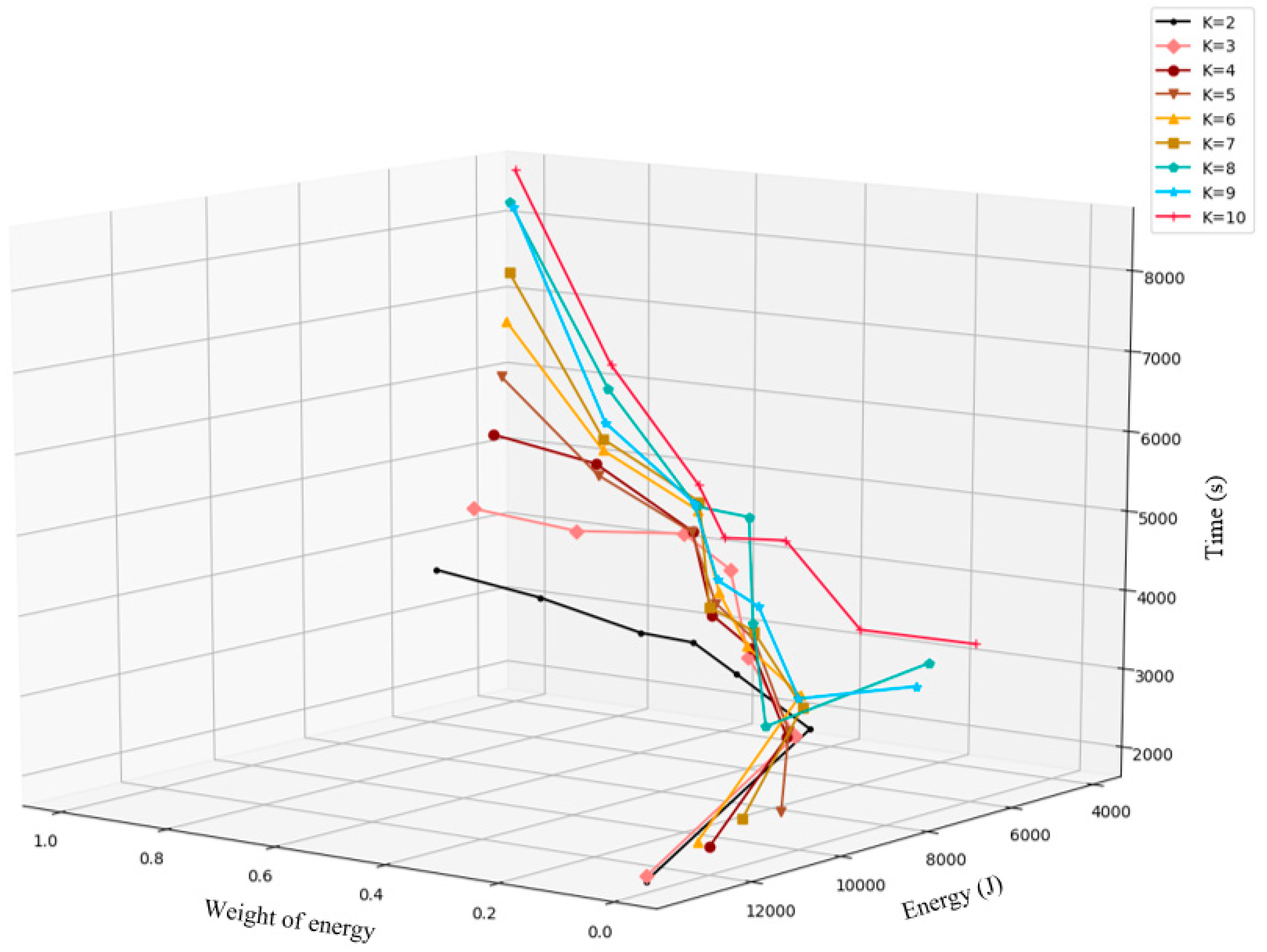
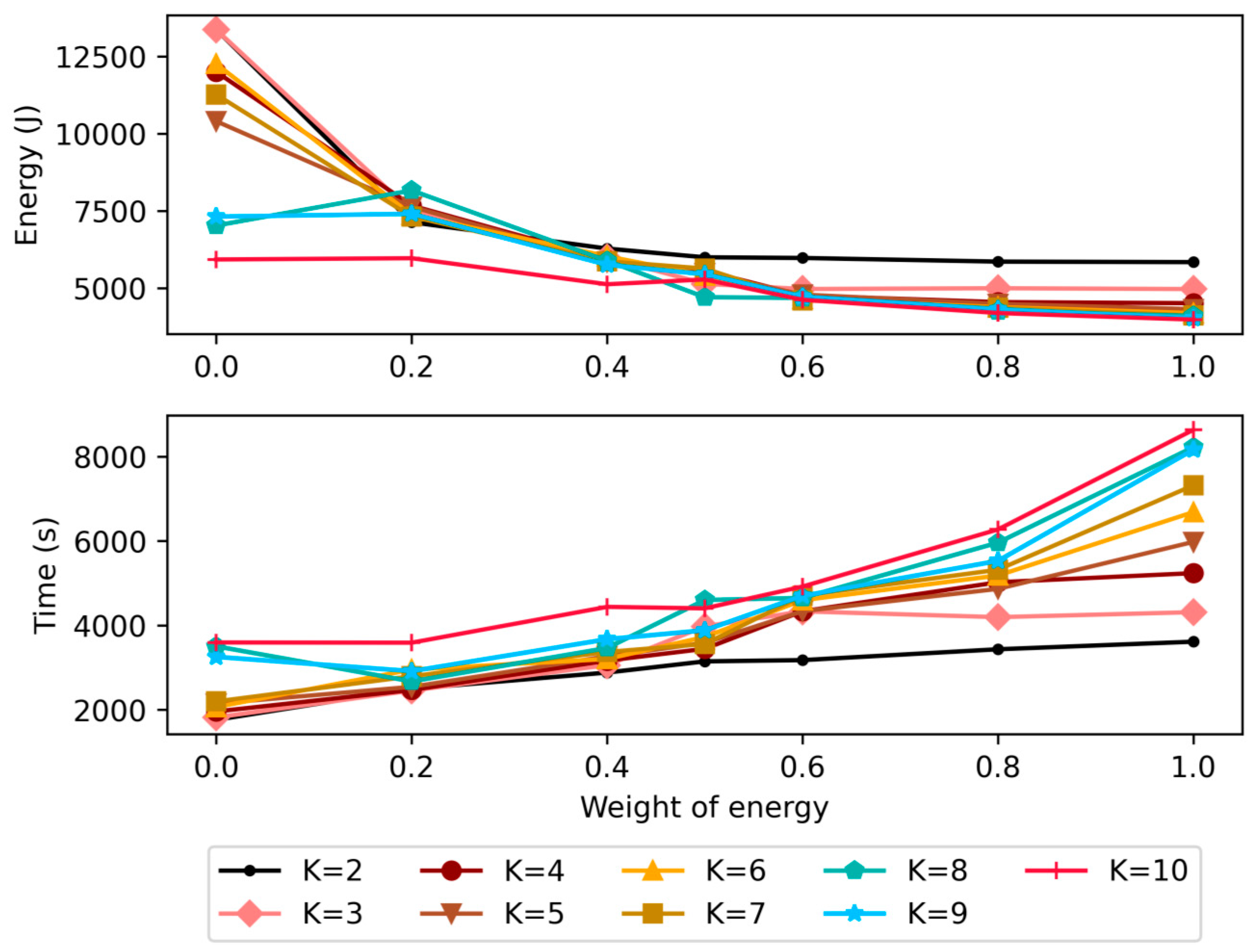
5. Lake Trial Results and Discussion

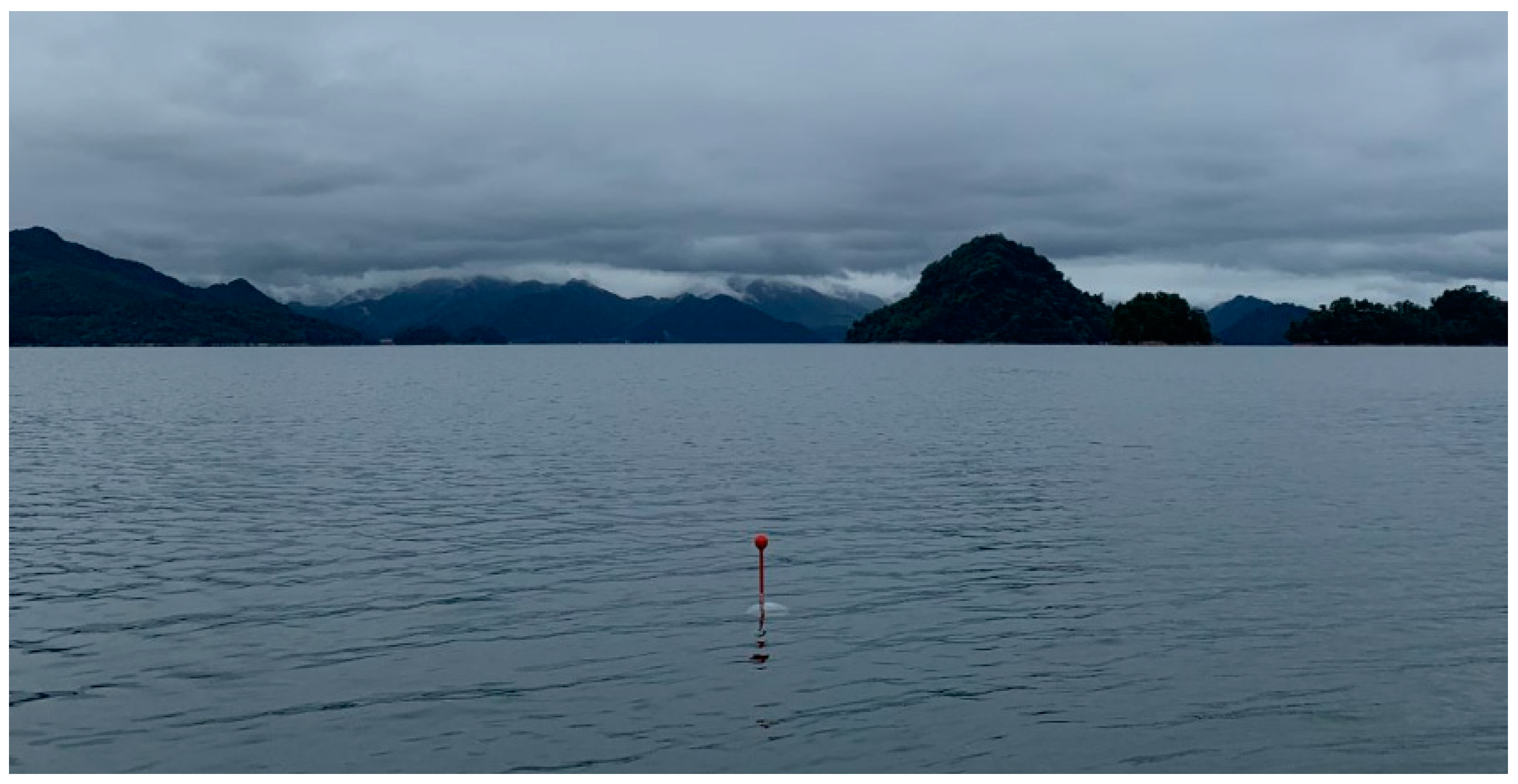
The above discussion shows that an inverse relation exists between energy and time. If a larger weight is assigned to energy, the energy consumption of the device will be reduced. However, the time spent in ascending will increase. Similarly, if time is assigned a larger weight, the ascent will be faster. A field experiment was conducted in Qiandao Lake in September 2020 for verifying the buoyancy regulation strategy (see Figure 10).
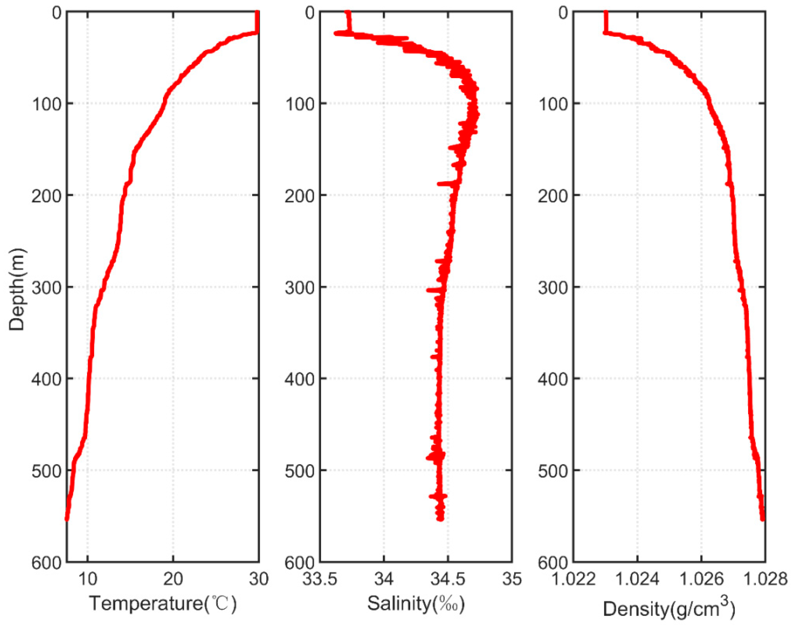
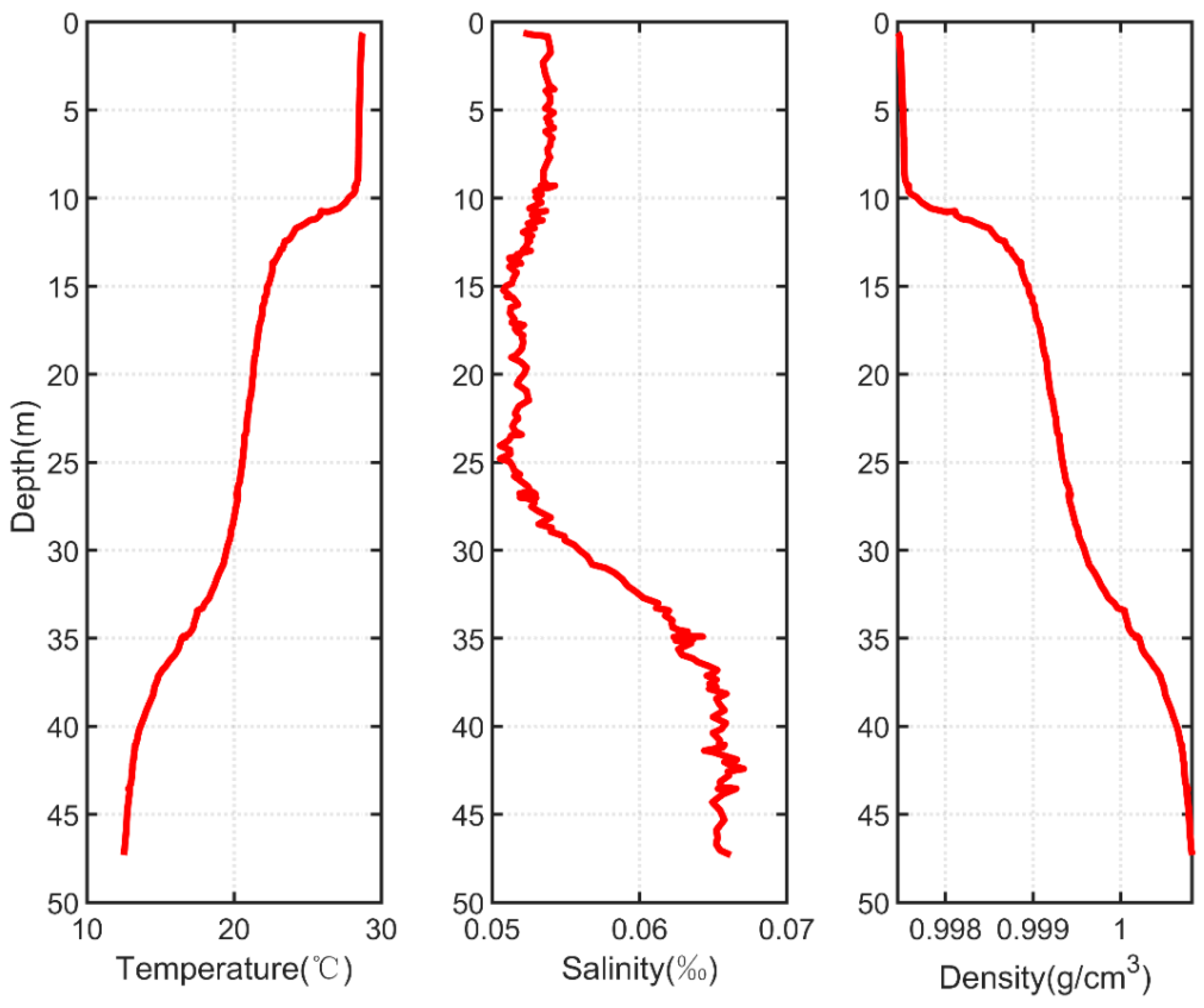
The depth of the site of the trial is 47.6 m. The depth profiles of temperature and salinity are shown in Figure 11. The temperature at the water surface was 28.8 °C, and that at a depth of 47.6 m was 12.5 °C. Salinity did not change significantly with depth as Qiandao Lake is a freshwater lake.
The main control chip of the ZJU-HUP is MSP430. It is responsible for the execution of the related actions, for example, turning on the motor and sending GPS (global positioning system) information. The sensor management board collects information from various sensors. A circuit board based on Arduino was added to the ZJU-HUP in this experiment. This circuit board can receive sensor data from the master chip and store it into an SD (secure digital) card. It is also connected to two Hall elements that measure the current of the buoyancy regulation system.
The buoyancy regulation strategy, after AGA optimisation, is described in Table 2. The strategy needs to account for an initial optimised depth of 40 m and a final optimised depth of 5 m. If the oil is pumped to the external bladder once, the HUP turns on the motor of the buoyancy regulation system at a depth of 40 m to ascend to a depth of 5 m all at once. If the oil is pumped to the external bladder twice, the HUP partially pumps oil out first at a depth of 40 m to reach the next depth of 9 m, and then at 9 m, it pumps the rest of the oil. If the oil is pumped to the external bladder three times, the HUP pumps oil at three depths (40, 12, and 7 m).
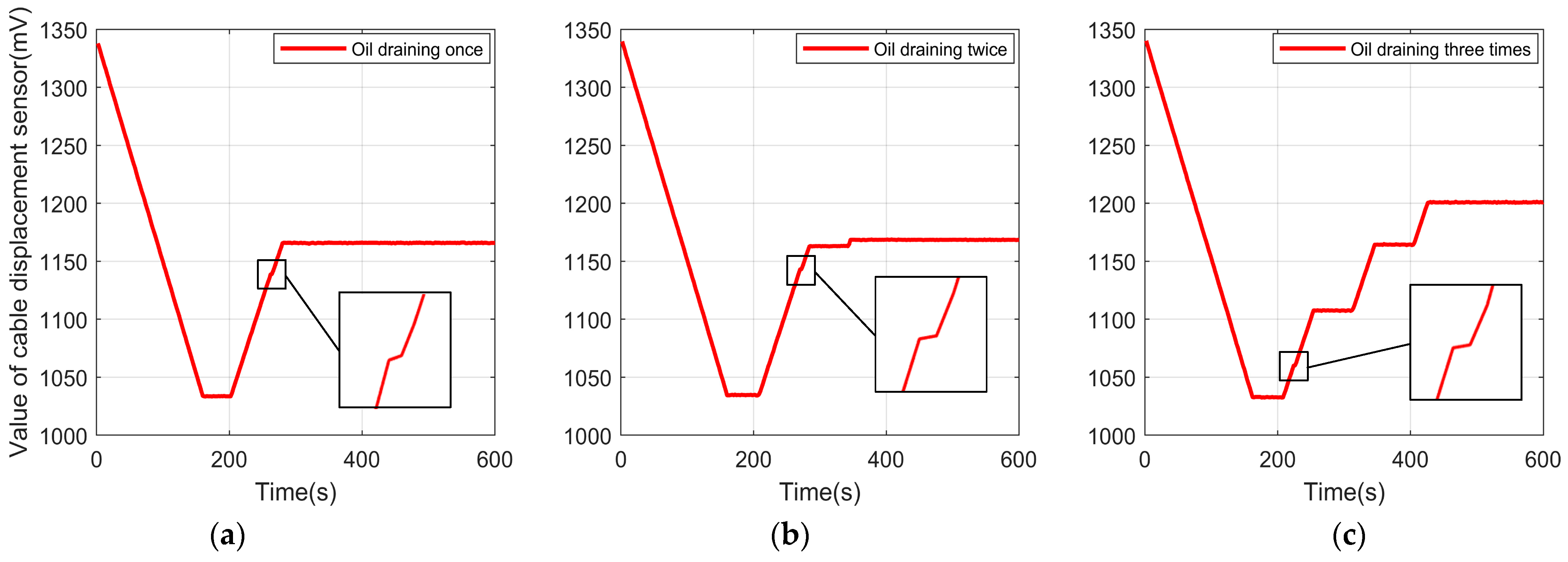
The cable displacement sensor is a device that can output the position of the piston in a cylinder. Using this sensor, the amount of oil in the external bladder can be determined by setting the position of the piston. The cable displacement sensor output voltage signal and the target voltage value can be calculated according to the amount of oil required. The piston positions at different stages during the overall process are listed in Table 3.
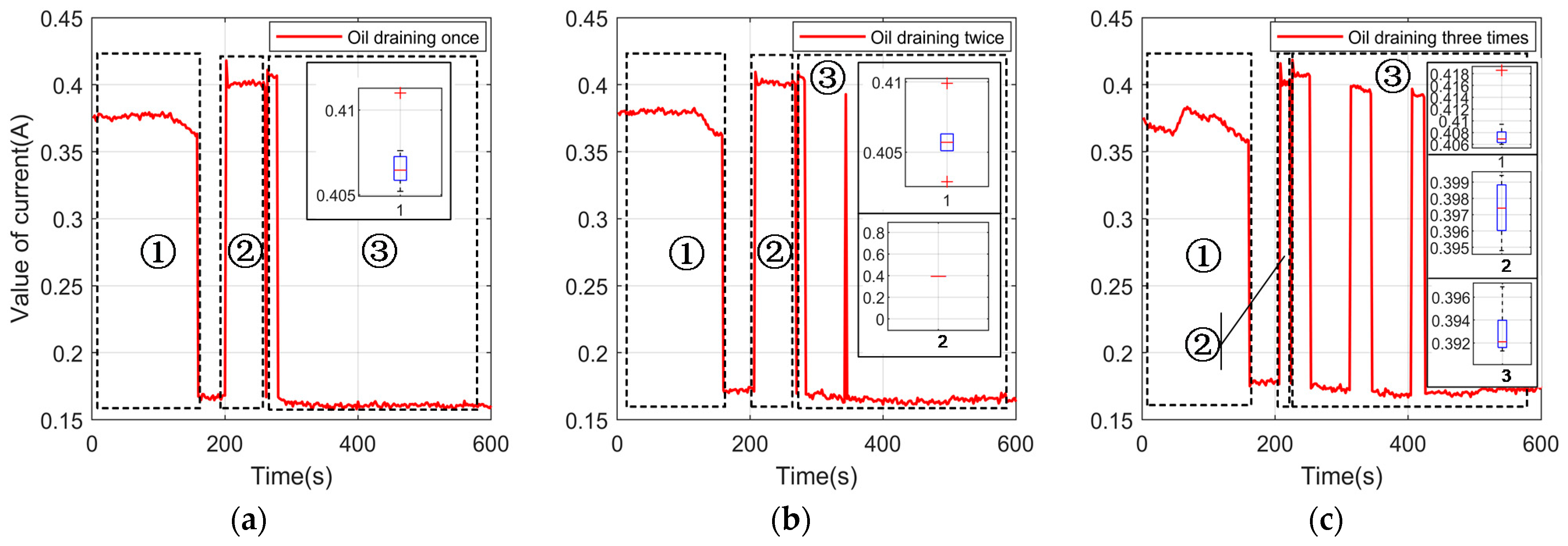
The value of the motor current during the trial is shown in Figure 12. The entire process is divided into three periods. The value of the cable displacement sensor is shown in Figure 13; the insets in the figure show a magnified view of the starting positions for the buoyancy regulation strategy. When the buoyancy regulation system starts pumping oil from the external bladder (①), the HUP begins to descend while simultaneously recording temperature, pressure, time, and current data. When a depth of 38 m is reached, the HUP starts pumping oil into the external bladder to increase the overall volume (②), so that it slows down gradually and then begins to ascend. The depth at which the HUP begins to pump oil out is calculated based on the kinematics and dynamics; calculations show that the maximum depth that the HUP can reach is 42 m. When the HUP returns to a distance of 2 m from the greatest depth, it first stops for 1 s and then starts to implement the buoyancy regulation strategy (③).
Two phenomena were noted in the experiment. First, during the experiment in which the oil was drained thrice, the output data of the pressure sensor underwent a fluctuation greater than 2 m, which caused the buoyancy regulation strategy to start earlier during the descent. However, this phenomenon did not affect the time and energy calculations. Next, the depths optimised by the AGA are listed in 
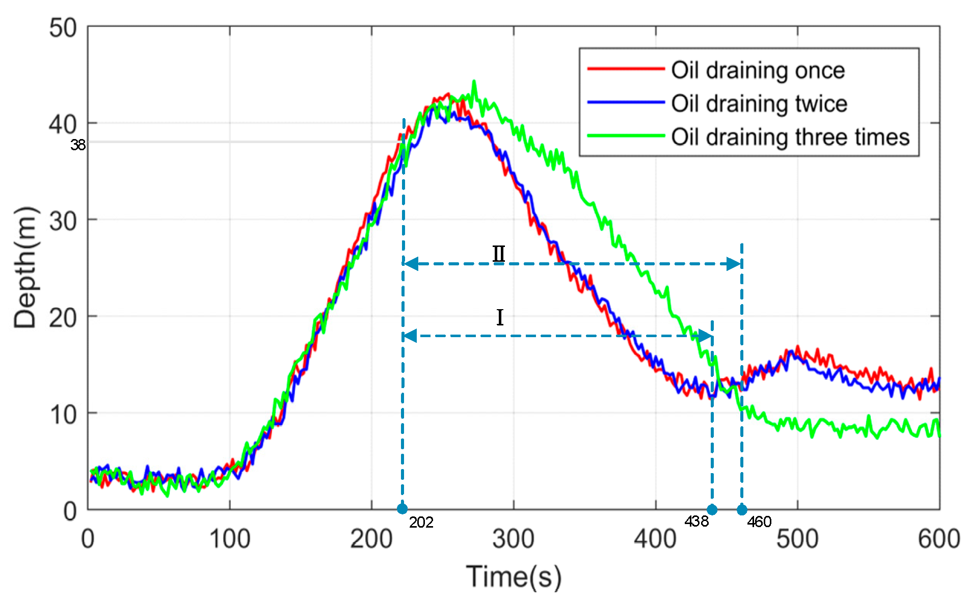
Table 2. However, owing to the complex underwater terrain of Qiandao Lake, security time protection is necessary between two consecutive depths and the protection was triggered because the ascent time between the two depths exceeded 1 min. So the buoyancy regulation strategy was not executed at the set depth. Therefore, this experiment is a preliminary verification of the buoyancy regulation strategy, but the contradictory relationship between energy and time can be obtained. Then, when the HUP is launched to perform tasks, overall time protection is necessary. If the operation time of HUP exceeds the predetermined time, the external bladder will be filled with oil, and then, the HUP will start ascending. Therefore, while the HUP was pumping oil out during the three oil-draining steps, overall time protection was triggered, and as a result, the final oil volume in the third experiment was more than that in each of the first two experiments, and the final depth achieved by the HUP float was smaller. However, according to the buoyancy regulation strategy, the minimum depth at which the HUP can reach is fixed. Therefore, according to the minimum depth the HUP reached in the first two experiments, the time when the buoyancy regulation strategy of the third experiment ends can be inferred. Thus, the range of the buoyancy regulation strategy of the three experiments can be obtained. Since the changes in the depth in the first two experiments are similar, the overall process of the buoyancy regulation strategy is both represented as Interval I. The process of the third experiment is represented as Interval II.
The optimisation results listed in Table 3 show that the target position of the first oil pumping is close to that of the second oil pumping. This makes the depth change of the oil draining twice similar to that of the oil draining once. From Figure 14, we can see that the time spent is 236 s in interval I and 258 s in interval II. The third experiment requires 9.32% more time than the first two experiments.
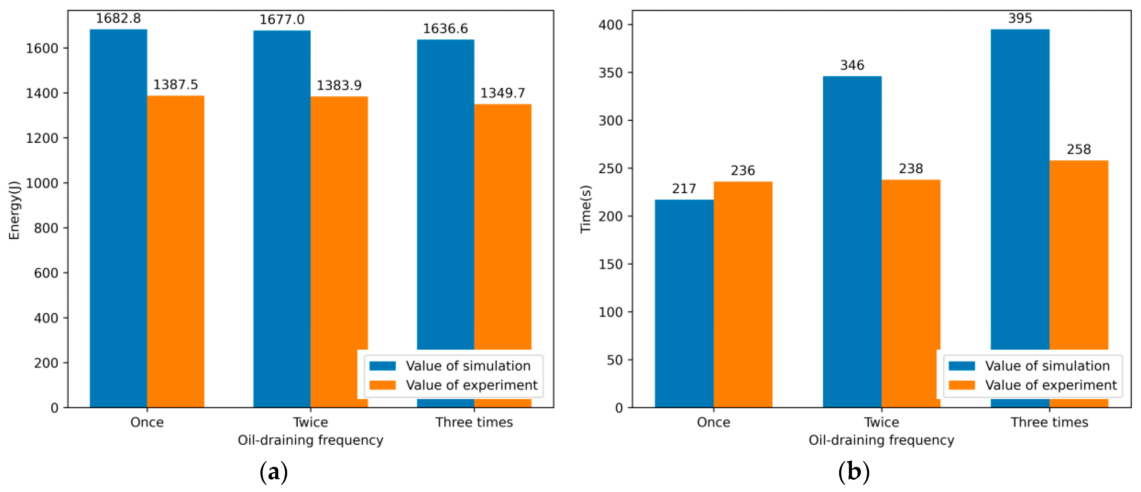
To analyse the current data more comprehensively, box diagrams were plotted based on the current value. The power of the motor changed when pumping oil at different depths, and as the depth increased, the energy consumed of the motor increased too. By calculating the energy for interval I and interval II, we can draw the conclusion that the energy consumed of oil draining twice is 0.26% less than that of oil draining once and the energy consumed of oil draining three times is 2.72% less than that of oil draining once.
The simulation results are compared with the experimental results, as shown in Figure 15. It can be observed that the simulation results are close to the experiment results, but there are also differences. For the energy in Figure 15a, the value of simulation is greater than the value of the experiment. This may be due to the inconsistency between pressure and depth caused by the system error of the pressure sensor. For the time in Figure 15b, the error between the simulation value and the experiment value may be caused by the experimental setup. Because there is no depth control in the experiment, the ZJU-HUP does not start to move from the depth of 40 m, but more than 40 m. This will make the speed greater than 0 at the depth of 40 m, which will lead to a reduction in the floating time.

6. Conclusions

In this paper, a buoyancy regulation strategy for underwater profilers is proposed. In this strategy, oil is pumped out several times instead of all at once. First, the relationship between the volume of the external bladder and the density difference was established, and that between the motor power and the depth was experimentally obtained. Then, a floating kinematics model of the profiler was established, and the depth of oil draining was optimised based on the AGA. Next, the buoyancy regulation strategy was numerically simulated using sea trial data for depths of 0–500 m. The fitness function was the smallest when the oil is pumped out four times under the condition that the weights assigned to power and time were both 0.5. Finally, the trial was performed at depths of 0–40 m in Qiandao Lake. During the ascent, the ascent time of oil draining thrice was 9.32% more than the ascent time of oil draining once, but the corresponding energy consumed was less by 2.72%. As the depth of the water area in this experiment is relatively shallow, the reduction of energy and the increase in time are not obvious. In addition, an appropriate depth control method should be studied and applied. Therefore, in subsequent research, we will verify the buoyancy regulation strategy with depth control in the sea trial to observe more significant numerical changes.

Author Contributions

Conceptualization, H.Z., P.Z., and Y.C.; Data curation, H.Z. and M.L.; Formal analysis, Y.H.; Funding acquisition, C.Y.; Methodology, H.Z.; Resources, Y.C.; Software, X.Z.; Writing—original draft, H.Z.; Writing—review and editing, H.Z. All authors have read and agreed to the published version of the manuscript.

Funding

This work was funded by National Natural Science Foundation of China (No. 51979246) and the Natural Science Foundation of Zhejiang Province of China (No. LY18E090003)

Data Availability Statement

The data presented in this study are available on request from the corresponding author.

Conflicts of Interest

The authors declare no conflict of interest.

References

  1. Guillerme, J.-B.; Couteau, C.; Coiffard, L. Applications for Marine Resources in Cosmetics. Cosmetics 2017, 4, 35. [Google Scholar] [CrossRef] [Green Version]
  2. Copping, A.E.; Hemery, L.G.; Overhus, D.M.; Garavelli, L.; Freeman, M.C.; Whiting, J.M.; Gorton, A.M.; Farr, H.K.; Rose, D.J.; Tugade, L.G. Potential Environmental Effects of Marine Renewable Energy Development—The State of the Science. J. Mar. Sci. Eng. 2020, 8, 879. [Google Scholar] [CrossRef]
  3. Fiorelli, E.; Leonard, N.E.; Bhatta, P.; Paley, D.A.; Bachmayer, R.; Fratantoni, D.M. Multi-AUV Control and Adaptive Sampling in Monterey Bay. IEEE J. Ocean. Eng. 2006, 31, 14. [Google Scholar] [CrossRef] [Green Version]
  4. Yu, J.; Zhang, A.; Jin, W.; Chen, Q.; Tian, Y.; Liu, C. Development and experiments of the Sea-Wing underwater glider. China Ocean Eng. 2011, 25, 721–736. [Google Scholar] [CrossRef] [Green Version]
  5. Webb, D.C.; Simonetti, P.J.; Jones, C.P. SLOCUM: An underwater glider propelled by environmental energy. IEEE J. Ocean. Eng. 2001, 26, 447–452. [Google Scholar] [CrossRef]
  6. Roemmich, D.; Johnson, G.; Riser, S.; Davis, R.; Gilson, J.; Owens, W.B.; Garzoli, S.; Schmid, C.; Ignaszewski, M. The Argo Program: Observing the global ocean with profiling floats. Oceanography 2009, 22, 34–43. [Google Scholar] [CrossRef] [Green Version]
  7. Asakawa, K.; Nakamura, M.; Kobayashi, T.; Watanabe, Y.; Hyakudome, T.; Ito, Y.; Kojima, J. Design Concept of Tsukuyomi —Underwater Glider Prototype for Virtual Mooring. In Proceedings of the OCEANS 2011 IEEE—Spain, Santander, Spain, 6–9 June 2011; pp. 1–5. [Google Scholar]
  8. Cao, J.; Lu, D.; Li, D.; Zeng, Z.; Yao, B.; Lian, L. Smartfloat: A Multimodal Underwater Vehicle Combining Float and Glider Capabilities. IEEE Access 2019, 7, 77825–77838. [Google Scholar] [CrossRef]
  9. Asakawa, K.; Kobayashi, T.; Nakamura, M.; Watanabe, Y.; Hyakudome, T.; Itoh, Y.; Kojima, J. Results of the First Sea-Test of Tsukuyomi: A Prototype of Underwater Gliders for Virtual Mooring. In Proceedings of the 2012 Oceans, Hampton Roads, VA, USA, 14–19 October 2012; pp. 1–5. [Google Scholar]
  10. Alexander, W. Design of a Low-cost Open-source Underwater Glider. engrXiv 2018. [Google Scholar] [CrossRef]
  11. Jones, C.P. Slocum Glider Persistent Oceanography. In Proceedings of the 2012 IEEE/OES Autonomous Underwater Vehicles (AUV), Southampton, UK, 24–27 September 2012; pp. 1–6. [Google Scholar]
  12. Yazji, J.; Zaidi, H.; Torres, L.T.; Leroy, C.; Keow, A.; Chen, Z. A Novel Buoyancy Control Device Using Reversible PEM Fuel Cells. In Proceedings of the ASME 2019 Dynamic Systems and Control Conference, Park City, UT, USA, 8–11 October 2019; p. V003T17A006. [Google Scholar]
  13. Um, T.I.; Chen, Z.; Bart-Smith, H. A novel electroactive polymer buoyancy control device for bio-inspired underwater vehicles. In Proceedings of the 2011 IEEE International Conference on Robotics and Automation, Shanghai, China, 9–13 May 2011; pp. 172–177. [Google Scholar] [CrossRef]
  14. Si, W.; Xue, Y.; Liu, Y.; Li, Z.; Xue, G. Energy Consumption Modeling and Sensitivity Analysis for Deep-Argo Otarriinae Profiling Float. Math. Problems Eng. 2020, 2020, 1–14. [Google Scholar] [CrossRef]
  15. Petzrick, E.; Truman, J.; Fargher, H. Profiling from 6000 meter with the APEX-Deep float. In Proceedings of the 2013 OCEANS—San Diego, San Diego, CA, USA, 23–27 September 2013; pp. 1–3. [Google Scholar] [CrossRef]
  16. MU, W.; ZOU, Z.; Zhenxing, H. A Control Strategy with Low Power Consumption for Buoyancy Regulation System of Submersibles. J. Xi’an Jiaotong Univ. 2018, 52, 44–49. [Google Scholar] [CrossRef]
  17. Liu, M.; Yang, S.; Li, H.; Xu, J.; Li, X. Energy Consumption Analysis and Optimization of the Deep-Sea Self-Sustaining Profile Buoy. Energies 2019, 12, 2316. [Google Scholar] [CrossRef] [Green Version]
  18. Zhou, P.; Yang, C.; Wu, S.; Zhu, Y. Designated Area Persistent Monitoring Strategies for Hybrid Underwater Profilers. IEEE J. Ocean. Eng. 2020, 45, 1322–1336. [Google Scholar] [CrossRef]
  19. Azzouz, A.; Ennigrou, M.; Said, L.B. Solving flexible job-shop problem with sequence dependent setup time and learning effects using an adaptive genetic algorithm. Int. J. Comput. Intell. Stud. 2020, 9, 18–32. [Google Scholar] [CrossRef]
  20. Jafar-Zanjani, S.; Inampudi, S.; Mosallaei, H. Adaptive Genetic Algorithm for Optical Metasurfaces Design. Sci. Rep. 2018, 8, 11040. [Google Scholar] [CrossRef] [PubMed]
  21. Chen, F.; Xu, S.; Zhao, Y.; Zhang, H. An Adaptive Genetic Algorithm of Adjusting Sensor Acquisition Frequency. Sensors 2020, 20, 990. [Google Scholar] [CrossRef] [PubMed] [Green Version]
  22. Srinivas, M.; Patnaik, L.M. Adaptive probabilities of crossover and mutation in genetic algorithms. IEEE Trans. Syst. Man Cybern. 1994, 24, 656–667. [Google Scholar] [CrossRef] [Green Version]
  23. Isdale, J.D.; Morris, R. Physical properties of sea water solutions: Density. Desalination 1972, 10, 329–339. [Google Scholar] [CrossRef]
Figure 1. Schematic diagram of the working process of an underwater profiler.
Jmse 09 00053 g001
Figure 2. Schematic diagram of the buoyancy regulation system.
Jmse 09 00053 g002
Figure 3. Schematic diagram of the experimental buoyancy regulation system.
Jmse 09 00053 g003
Figure 4. Motor power and speed of oil discharge curves at different depths.
Jmse 09 00053 g004
Figure 5. Implementation process of the buoyancy regulation strategy.
Jmse 09 00053 g005
Figure 6. Depth profiles of temperature, salinity, and density in the South China Sea.
Jmse 09 00053 g006
Figure 7. Three-dimensional graph of energy and time variation with different weights.
Jmse 09 00053 g007
Figure 8. Two-dimensional graph of energy and time variation with different weights (top: energy varying with different weights; bottom: time varying with different weights).
Jmse 09 00053 g008
Figure 9. (a) The fitness value against the oil-draining frequency; (b) Convergence curve of the fitness value.
Jmse 09 00053 g009
Figure 10. Lake trial conducted at Qiandao Lake.
Jmse 09 00053 g010
Figure 11. Depth profiles of temperature, salinity and density in Qiandao Lake.
Jmse 09 00053 g011
Figure 12. (a) Value of current when the oil is draining once; (b) Value of current when the oil is draining twice; (c) Value of current when the oil is draining three times.
Jmse 09 00053 g012
Figure 13. (a) Value of the cable displacement sensor when the oil is draining once; (b) Value of the cable displacement sensor when the oil is draining twice; (c) Value of the cable displacement sensor when the oil is draining three times.
Jmse 09 00053 g013
Figure 14. Depth variation during the experiment.
Jmse 09 00053 g014
Figure 15. Comparison of simulation results and experiment results. (a) Energy comparison of simulation results and experiment results; (b) Time comparison of simulation results and experiment results.
Jmse 09 00053 g015
Table 1. Main specifications of Zhejiang University hybrid underwater profiler (ZJU–HUP).
FeatureDescription
Hull length2300 mm
Weight82 kg
Buoyancy regulationGear pump
Maximum Volume of the bladder1.8 L
Table 2. Optimisation results based on adaptive genetic algorithm.
Oil Draining FrequencyFirst Depth (m)Second Depth (m)Third Depth (m)Energy (J)Time (s)
Once40--1682.8217
Twice409-1677346.27
Three times401271636.6394.56
Table 3. The value of the cable displacement sensor corresponding to the depth interval.
Oil Draining FrequencyInitial Position (mV)First Position (mV)Second Position (mV)Third Position (mV)
Once10331165--
Twice103311611165-
Three times1033110611631165
Publisher’s Note: MDPI stays neutral with regard to jurisdictional claims in published maps and institutional affiliations.

