1. Introduction
According to the fifth Assessment Report (AR5) published by the IPCC [
1], the medium-term and long-term countermeasures are expected to accommodate the possible impacts of climate change. The Ministry of the Environment (MOE) in Japan has discussed planning for a climate change adaptation policy. Some research projects in Japan such as S-8 [
2] have forecast climate change effects by region and provide support for adaptative countermeasures. Assessment of climate change effects and the effectiveness of adaptation measures based on nationwide and regional climate change projection are needed.
Numerous attempts have been undertaken to evaluate the economic effects of climate change. Their evaluation methods are classifiable into two approaches: A partial equilibrium approach and a general equilibrium approach. The former method includes a travel cost method (TCM) and a contingent valuation method (CVM). These methods have been applied in some studies to quantify the economic value of the natural environment and ecosystems and the value of statistical life. Since these methods are partial equilibrium approaches, however, economic effects of changes in natural environment by climate change and environmental conservation policies on the whole economy cannot be captured. On the other hand, the latter method has a computable general equilibrium (CGE) analysis. Since a computable general equilibrium model explicitly formulates an objective function in economic agent, direct effects of climate change on economic activities of agent can be captured. In addition, since a CGE model treats all markets in the economy, indirect effects of climate change on the entire economy through changes in the behavior of agents can be captured. Using a CGE model, however, to measure the economic effects of climate change on the natural environment and ecosystems, formulation of the effects on them and estimation of their parameters in a model are necessary. As described above, numerous studies of economic evaluation of climate change have separately been analyzed by two approaches. Therefore, comprehensive assessments in a general equilibrium framework must be made through explicit linkage between a partial equilibrium approach and a general equilibrium approach.
By applying a recreation demand function to a general equilibrium model, for water reallocation issues in Nevada in the United States, Seung et al. [
3] analyzed the effects of water reallocation on some recreation sectors and the agriculture sector. However, since the recreation demand function used in their study does not account for the generalized transportation cost, it is not consistent with a utility function. Ciscar et al. [
4] comprehensively evaluated the economic and physical effects of climate change on the natural environment, ecosystem, and human society in Europe by treating four sectors as physical effect terms: Agriculture, coastal zone, flood, and tourism. Although their study produced estimates of respective physical effects from projected climate data under conditions of socioeconomic scenarios, and evaluated the projected economic effects by the economic model, it has no theoretical consistency between estimates of physical effect terms and economic models. In a general equilibrium analysis of waste problems in Japan, Miyata [
5] derived a utility function consistent with a pre-formulated demand function from solving the integrability problem, and integrated externalities such as waste into a CGE model. For the sandy beach loss caused by climate change, Sakamoto and Nakajima [
6] and Nakajima and Sakamoto [
7] developed a CGE model that has a utility function consistent with a recreation demand function in a travel cost method by solving the integrability problem. Then, we extend the mode of describing the framework by Nakajima and Sakamoto [
7] to simulate more realistic climate change scenarios.
In Japan, although numerous studies such as those of Mimura et al. [
8] and Udo et al. [
9] have been made of the physical effects of sea level rise and the beach loss caused by climate change, little is known about the economic effects of beach loss and adaptation strategies against climate change. From
Table 1, Ohno et al. [
10] and Sao et al. [
11] evaluated recreation values for a sandy beach in Japan using a travel cost method. The former used beach loss rates calculated by Mimura et al. [
8] and estimated the prefectural damage cost of a sandy beach. The latter used beach loss rates by Udo et al. [
9], and evaluated not only the prefectural damage cost but also the effect of adaptation measures to restore a sandy beach. Since both studies were based on a partial equilibrium approach, they were unable to treat effects on prices and income caused by changes in environmental quality attributable to climate change. On the other hand, Sakamoto and Nakajima [
6], Nakajima and Sakamoto [
7], and Sao et al. [
11] estimated beach loss damage costs attributable to climate change using a CGE model incorporating a utility function consistent with a recreation demand function in the travel cost method. However, since these studies used future projections by Mimura et al. [
8], their economic assessments of beach loss became outdated. Although Sao et al. [
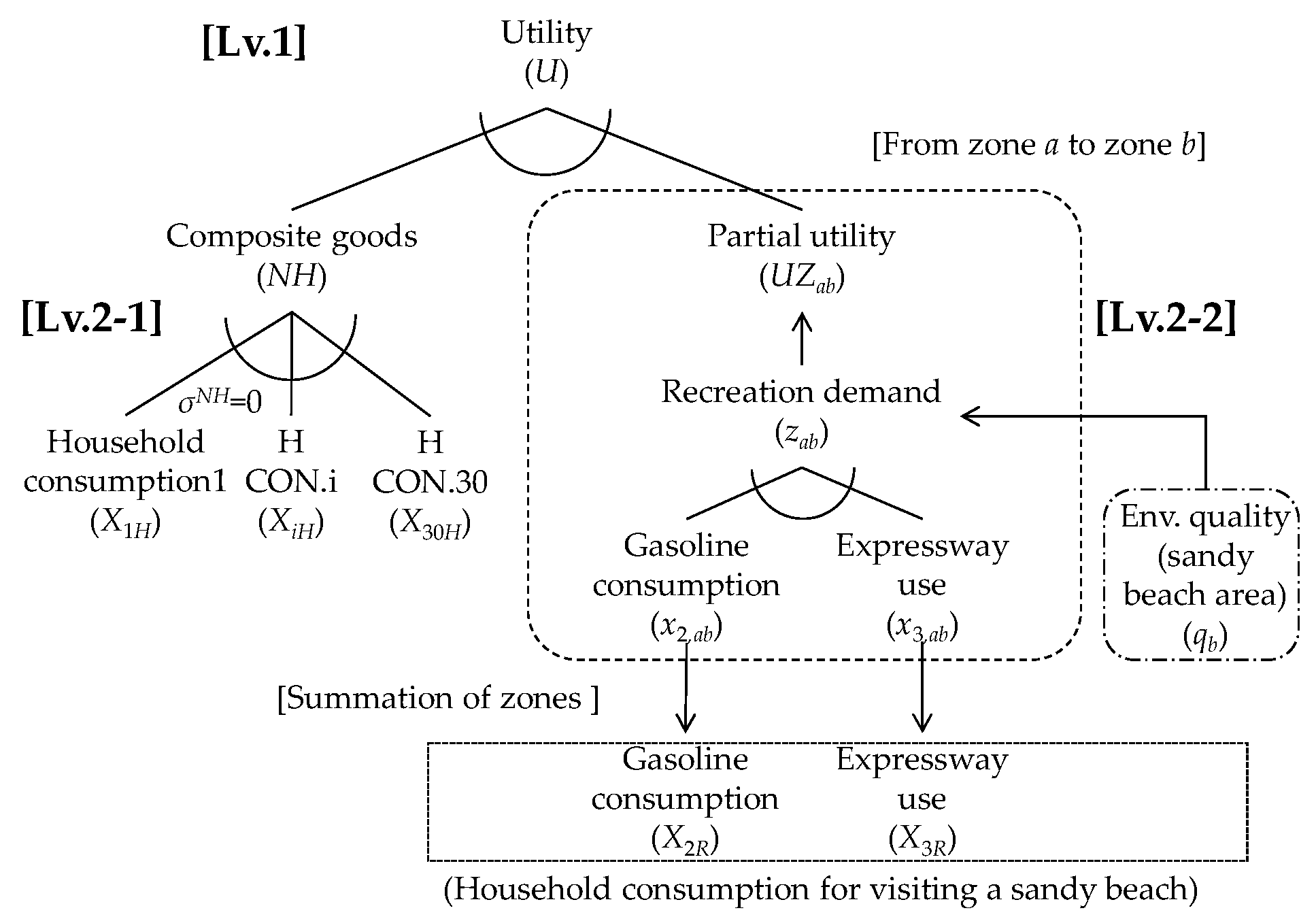
11] evaluated adaptation measures for beach loss, their CGE model in these studies had only three goods: Composite goods, gasoline, and an expressway used to visit a sandy beach for recreation. As one might expect, their model framework was quite unrealistic.
Therefore, we sought to measure economic effects of changes in environmental quality attributable to climate change in Japan. Results were obtained using a CGE model that integrates a utility function with environmental quality factors as an independent variable derived from a recreation demand function in a travel cost method (TCM), we aim to estimate the damage cost of beach loss in each prefecture and in Japan and to evaluate the economic effectiveness of hypothetical adaptation measures to restore sandy beaches.
4. Conclusions
To assess the economic effects of changes in environmental quality caused by climate change in Japan, we used a computable general equilibrium model that integrates a utility function with environmental quality factors as independent variables derived from a recreation demand function in a travel cost method. Results show the estimated damage costs of beach loss in Japan and in the respective prefectures. We evaluated the economic effectiveness of hypothetical adaptation measures to restore sandy beaches. The findings obtained from this study are presented below.
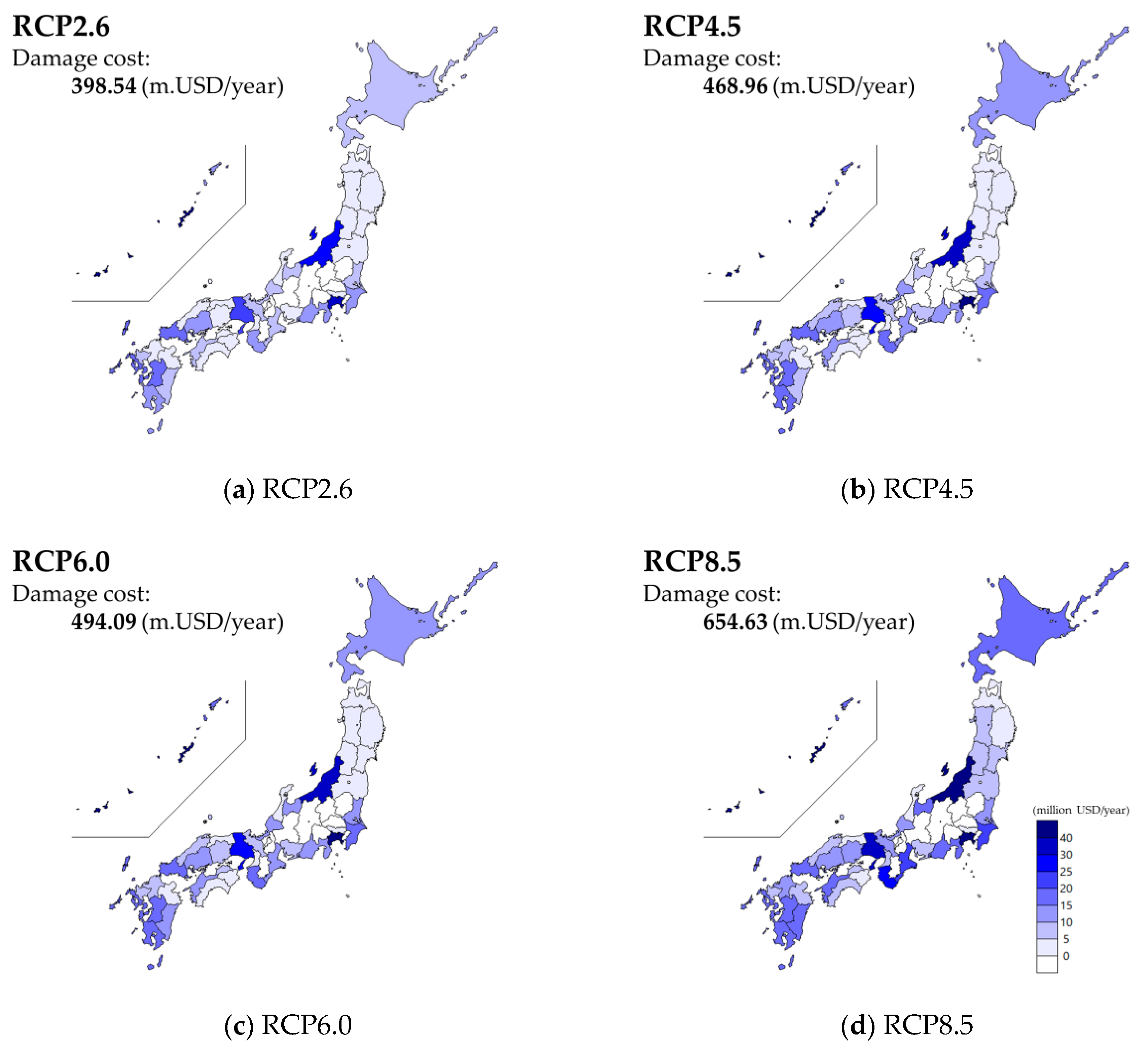
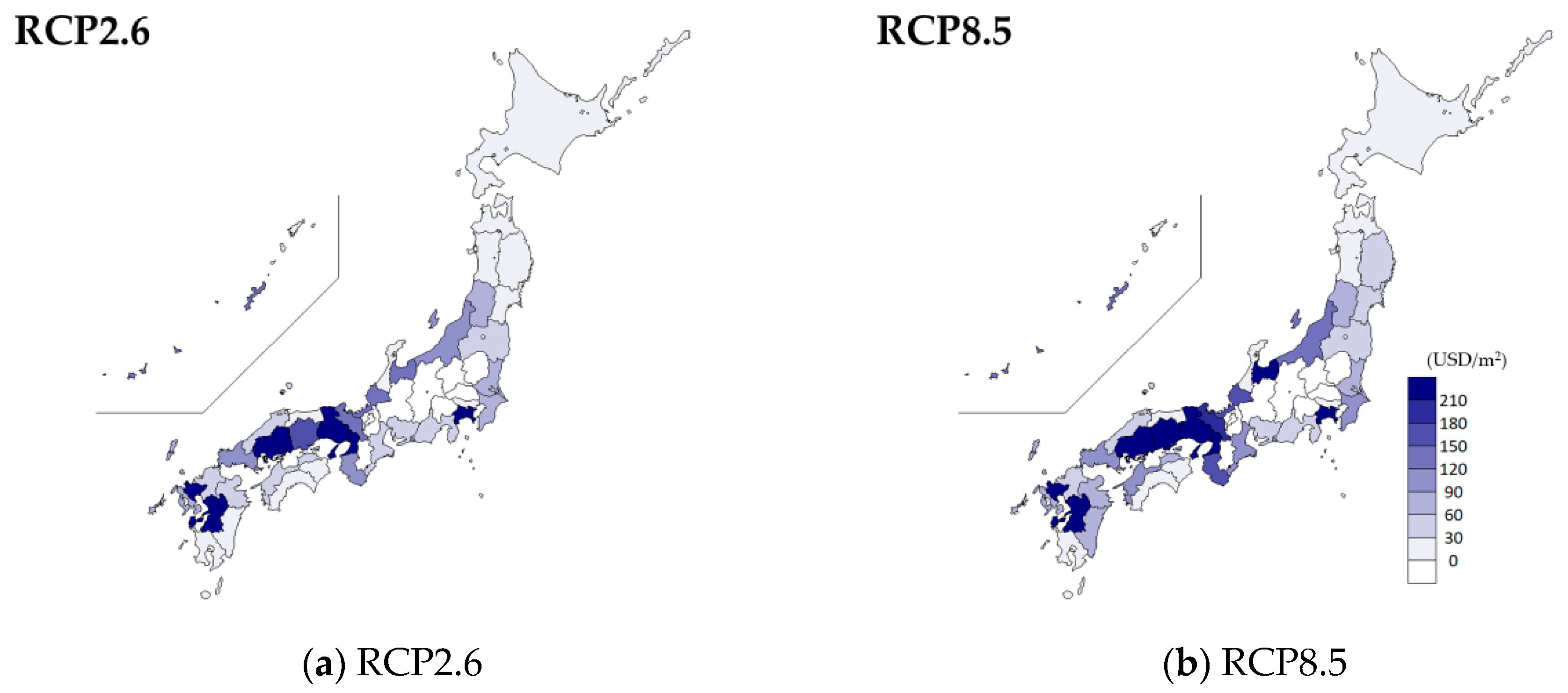
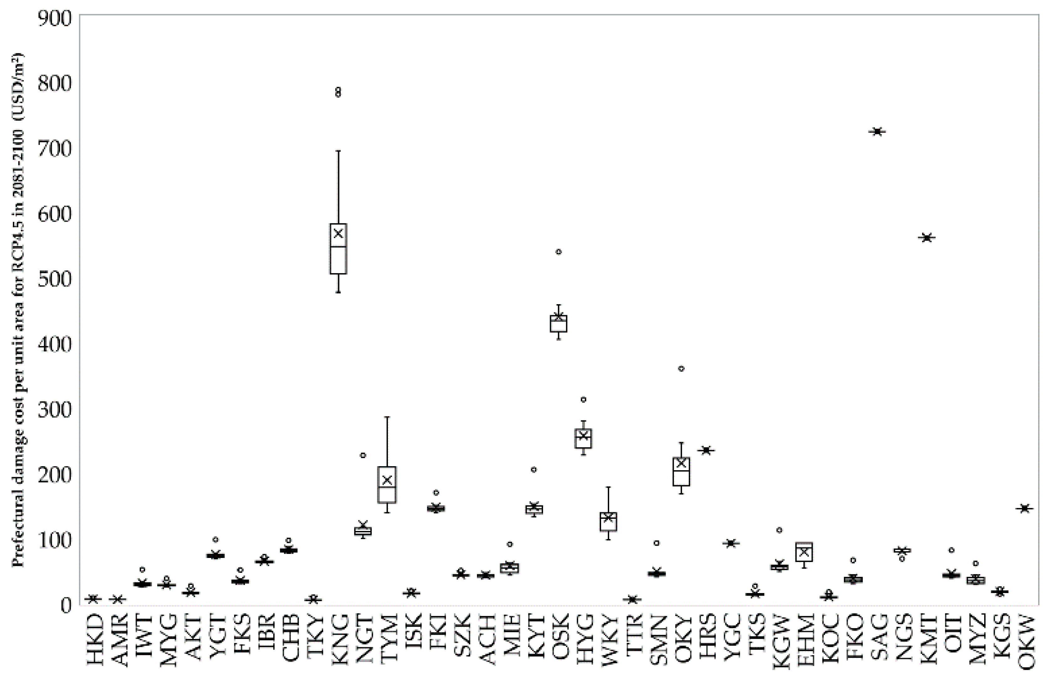
Higher future temperatures will cause higher damage costs of sandy beaches. In 2081–2100, we estimated damage costs as 398.54 million USD per year for RCP2.6, 468.96 (m.USD/year) for RCP4.5, 494.09 (m.USD/year) for RCP6.0, and 654.63 (m.USD/year) for RCP8.5, respectively.
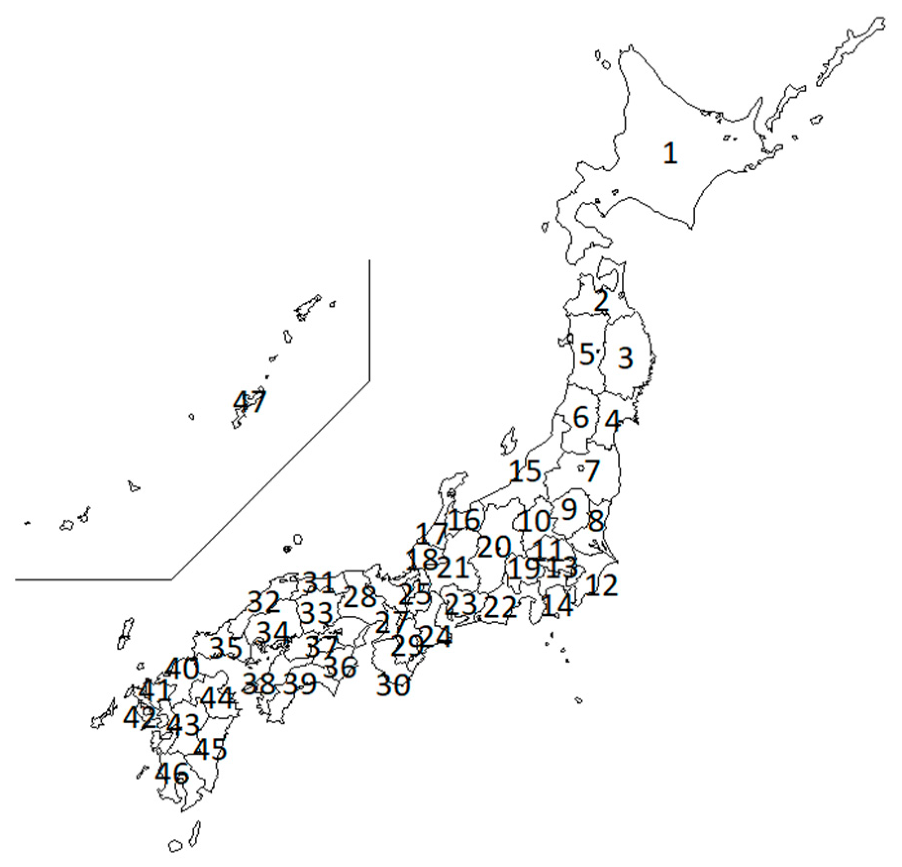
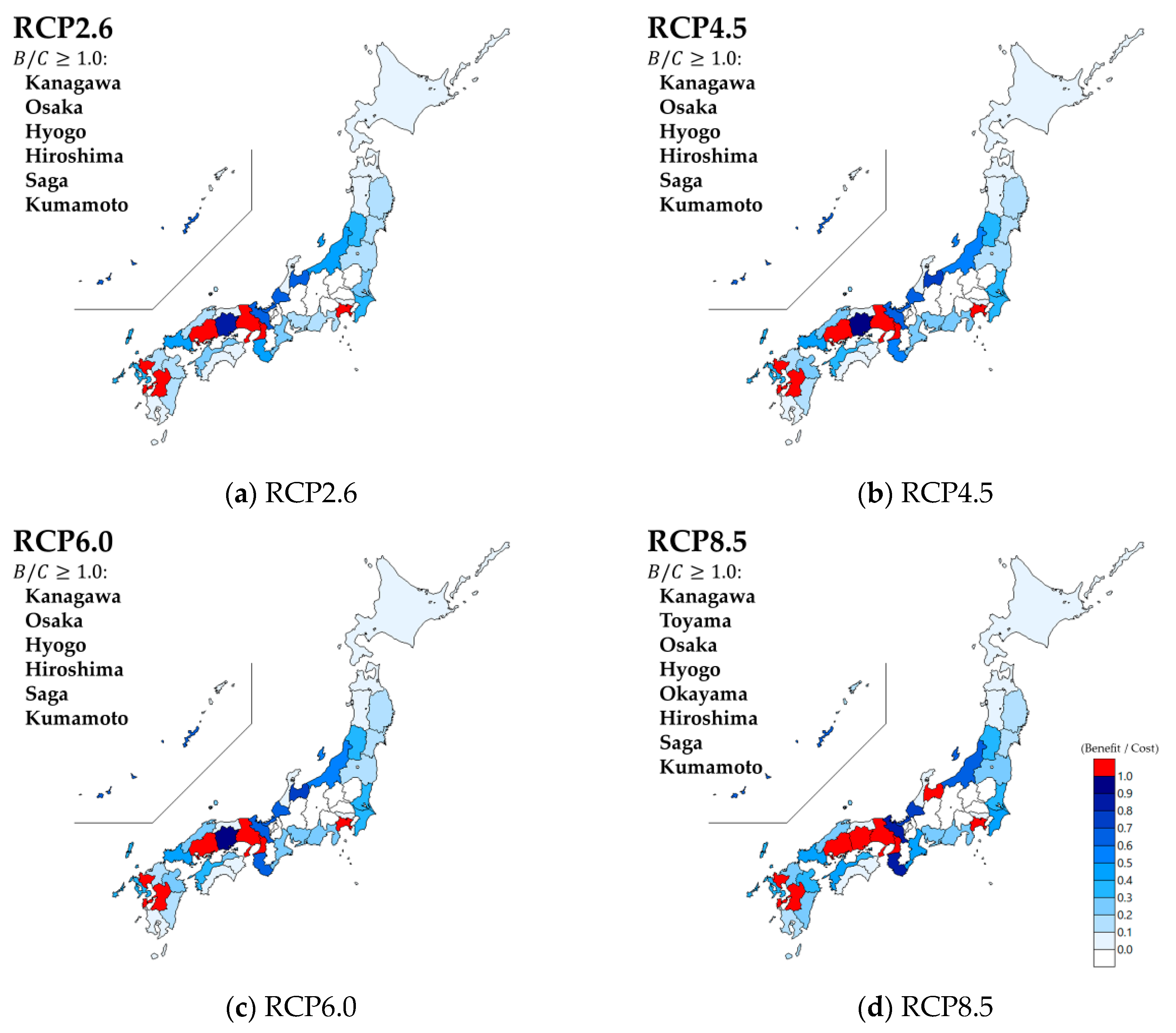
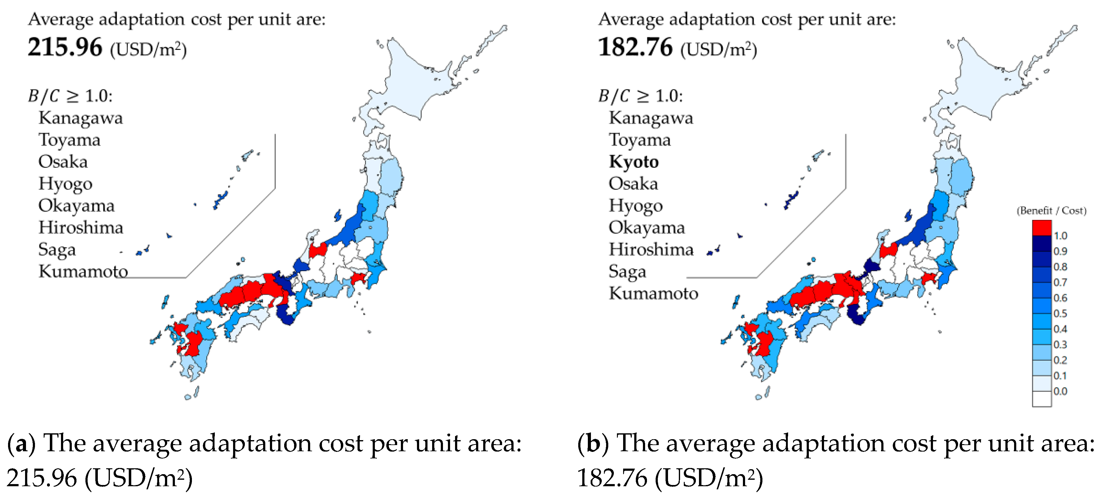
For all RCPs, six prefectures for which the cost–benefit ratio exceeds 1.0 were Kanagawa, Osaka, Hyogo, Hiroshima, Saga, and Kumamoto.
Higher future temperatures will bring high numbers of prefectures for which adaptation measures are cost–effective. Especially for four prefectures along the Inland Sea, which are Osaka, Hyogo, Okayama, and Hiroshima, our hypothetical adaptation measure of an artificial beach enhancement is expected to be quite effective as a public works project.
Further examinations can be expected to support further discussion. First, since we were unable to treat the adaptation cost endogenously, we will incorporate endogenous adaptation costs into our CGE model and evaluate the effectiveness of some adaptation measures. Secondly, since we evaluated only the recreation value (use value) estimated using TCM, we expect to develop a CGE model incorporating evaluation methods of non-use values.

 ,
, 


