Seasonal Dynamic of CDOM in a Shelf Site of the South-Eastern Ligurian Sea (Western Mediterranean)

Abstract

Chromophoric dissolved organic matter (CDOM) is the fraction of the Dissolved Organic Carbon (DOC) mainly absorbing UV and blue radiation, influencing water optical properties, light availability for primary production, and water-leaving radiance. In open seas, phytoplankton is the main source of organic carbon and CDOM. Despite this, the direct or indirect phytoplankton role in CDOM production is not yet fully clarified. From studies about the relationship between CDOM and phytoplankton biomass as Chlorophyll a (Chl) in the epipelagic layer, positive correlations have been highlighted with regional differences and high levels of variability. Seven years of seasonal dynamic and vertical distribution of CDOM in the Ligurian Sea continental shelf waters have been analyzed in order to evidence the main environmental and/or biological factors determining CDOM dynamic, focusing on the CDOM/Chl relationship. CDOM optical properties (absorption at 440 nm, a_CDOM (440), and spectral slope, S) allowed to distinguish different pools and to debate their origin. Four different pools were characterized and two of them were directly or indirectly related to phytoplankton biomass and taxonomic composition. Nevertheless, CDOM/Chl confirm a high level of variability These findings suggest some inputs to improve Mediterranean satellite estimates of Chl and CDOM, such as the seasonal differentiation of optical properties, especially S and CDOM/Chl relationships.

1. Introduction

Chromophoric dissolved organic matter (CDOM or ‘yellow substance’) is operationally defined as the group of absorbing substances that passes filters of 0.2 µm pore size [1]. CDOM is an important fraction of the Dissolved Organic Matter (DOM) in natural waters (10–90%, [2]) and it plays an important role in the ocean Carbon cycle [3]. CDOM can influence several marine processes: attenuation of UV radiation, thus making it less harmful to organisms, nutrient availability [4], light-dependent processes [5] and primary production [6,7], or optical properties as the intensity and the spectral features of water-leaving radiance [8,9].

For a long time, the importance of CDOM in ocean optics and biogeochemical studies has been known only for coastal ecosystems where runoff from land brings terrestrial CDOM so that its concentration is inversely correlated with salinity, and for areas such as the Baltic and polar seas where its concentration is very high [1,10,11,12]. Even though the importance of CDOM in open ocean and oligotrophic waters has been poorly considered. This is also due to the difficulties of measuring CDOM spectral light absorption coefficient with standard laboratory spectrophotometers, because of the low optical density of CDOM in natural seawater, especially in the oligotrophic ones. Thanks to extended programs of measurements and remote sensing studies, the relevance of detecting and monitoring CDOM has also been recently highlighted for oligotrophic environments [13,14] emphasizing that in these waters CDOM is the most important component for the absorption of submarine radiation from blue to UV spectral regions [15].

After early uncertainty surrounding the origin of marine CDOM, it was clear that, away from river-dominated margins and in open ocean areas, in situ phytoplankton primary production is the ultimate source of CDOM. Despite this, the role of phytoplankton in CDOM production is not yet fully clarified. Processes that release or recycle phytoplankton cell contents, such as sloppy feeding by grazers, viral lysis, excretion of metabolites by bacteria and zooplankton or exudation of mucus and other extracellular secretions, play a major role in production of CDOM [16]. Then, phytoplankton, directly or indirectly, is involved in many processes of excretion/degradation and likely plays a major role in the production of CDOM.

Most of the organic substance dissolved in the sea derived from phytoplankton is biologically labile and has a rather short life span, however a portion is not immediately mineralized and is transformed (biologically and abiologically) into resistant organic material and creates the large oceanic reservoir of CDOM. Thanks to this property, the fraction that absorbs UV has been and is used as a tracer of the water masses.

Many authors [17,18,19] studied the relationship between CDOM and phytoplankton biomass as chlorophyll a (Chl) in the epipelagic layer. In many types of water, a positive correlation has been found, despite regional difference in the ratio CDOM/Chl and high level of variability. The knowledge of the relationships between CDOM and Chl emerges as one of the crucial aspects to be foreseen in the development of algorithms for satellite estimate of Chl.

In the context of ocean optics, high CDOM contents can confound standard ocean colour algorithms used for the retrieval of biogeochemical variables, particularly Chl. This is the case of the Mediterranean Sea where CDOM absorption coefficients were found to be higher than in other oceans for a given chlorophyll concentration [18]. Since the first utilizations of remote sensing in the Mediterranean Sea, it was clear that global empirical algorithm to retrieve Chl using the blue/green reflectance bands ratio overestimates the actual concentration [18,20,21,22,23,24,25]. Lee and Hu, [26], hypothesized an unusual high CDOM concentration for a typical Case 1 oceanic condition by the analysis of the optical characteristics of the Mediterranean waters from satellite data. Then, Morel and Gentili [18] confirmed this hypothesis assessing indirectly CDOM concentrations by the analysis of the errors in Chl estimates, which were attributed to a higher CDOM concentration with respect to the open ocean. These differences can be ascribed to the inputs of terrigenous CDOM, linked to the characteristics of the semi-enclosed basin of the Mediterranean Sea [18].

Currently, direct measurements of CDOM concentration in the epipelagic layer across the Mediterranean Sea are available [27,28,29,30,31,32,33,34] and some direct knowledge about the concentration and dynamic of CDOM for some coastal and offshore site has been obtained.

In the present study, about seven years seasonal dynamic and vertical distribution of CDOM in the Case 1 waters of a Mediterranean Sea shelf site were analyzed. The production and loss of CDOM were investigated to describe the main features and causes of these processes, to understand the relationships between biological or physical-chemical transformation (seasonal structure of the water column) and autochthonous production vs. terrigenous inputs. Particular attention was focused on: relationships between CDOM and phytoplankton biomass, taxonomic, and size structure composition; CDOM optical properties in the context of an improvement of Mediterranean regional satellite algorithms.

2. Materials and Methods

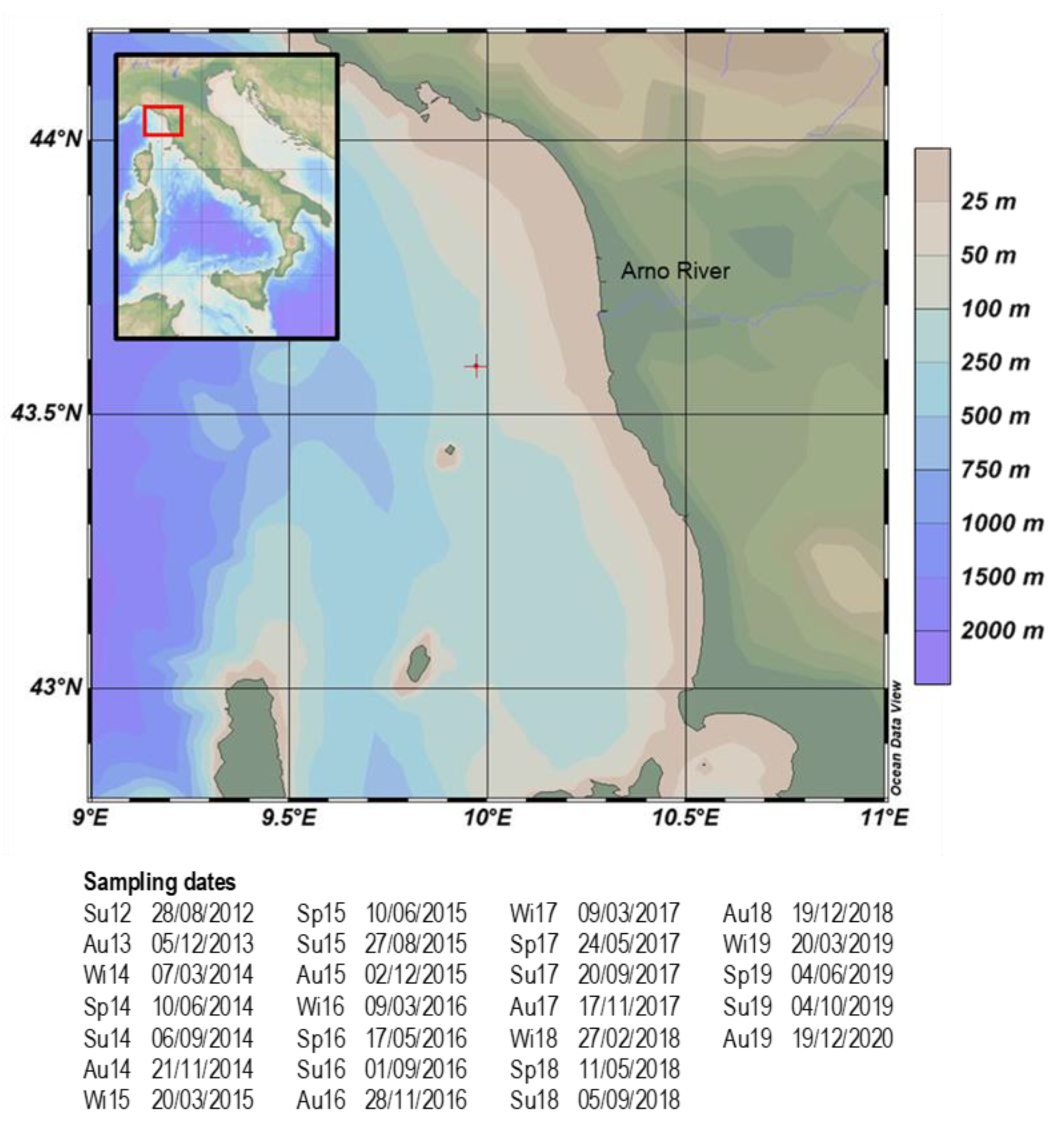
2.1. Study Area

The sampling site is located in the Southeastern Ligurian Sea at 43°37′35″; 9°59′18″, about 23 km from the Tuscany coast on a depth of about 100 m. This site is located south of the Arno river mouth and, considering the distance from the estuary and the prevailing South–North currents, only in the case of exceptional river flows can it be directly affected by the freshwater input, even though indirect influences are conceivable (Figure 1).

2.2. Sampling

The site was sampled in summer 2012 and thereafter with seasonal frequency from autumn 2013 to summer 2019. At each campaign Conductivity, Temperature and Depth (CTD, Sea Bird Electronics, Bellevue, WA, USA, 19v2plus) plus Photosynthetic Available Radiation (PAR) (Satlantic, Halifax, NS, Canada) profiles were carried out. PAR (%) profiles were obtained from contemporaneous in air (at sea surface) and underwater PAR measurements; the depth at which PAR was 1% of the superficial one is defined euphotic depth (z_eu). Seawater samples were collected at five depths (0.5, 12.5, 25, 50, and 70 m) by means of 12 L Niskin bottles, for a total of 120 samples.

2.3. Phytoplankton Pigments and Taxonomic Composition

Subsamples for pigments analysis (4 L) were filtered on GF/F Whatman filters (47 mm) and stored at −80 °C for not more than 1 month before analysis. Filters were homogenized in 90% acetone solution and the extracts were analyzed after 24 h (High Performance Liquid Chromatography, HPLC, SHIMADZU Class VP10, Kyoto, Japan) to determine the concentration of chlorophyll-a (Chl, mg·m⁻³) and seven diagnostic pigments [35,36]. Relative proportions of pico (<2 µm), nano (2–20 µm), and microphytoplankton (20–200 µm) were computed following [37,38]:

%picophytoplankton = 100(0.86[Zeaxanthin] + 1.01[Chlb + Divinyl-Chlb])/DP

(1)

%nanophytoplankton = 100(0.60[Alloxanthin] + 0.35[19′Butanoylfucoxanthin] +
+1.27[19′Hexanoyloxyfucoxanthin])/DP

(2)

%microphytoplankton = 100(1.41[Fucoxanthin] + 1.41[Peridinin])/DP

(3)

where DP is the sum of the concentrations of diagnostic pigments:

DP = 1.41[Fucoxanthin] + 1.41[Peridinin] + 0.60[Alloxanthin] + 1.27[19′Hexanoyloxyfucoxanthin] +
+0.35[19′Butanoylfucoxanthin] + 0.86[Zeaxanthin] + 1.01[Chlb + Divinyl-Chlb]

(4)

For the taxonomic analysis of phytoplankton, subsamples of 500 mL were collected, fixed with neutralized formalin (final concentration 1%) and stored in dark glass bottles. Subsamples of variable volumes were observed under an invertoscope (Zeiss IM35, Oberkochen, Germany, phase contrast, 40×) after sedimentation, following standard methods [39].

2.4. CDOM Absorption Measurements

Seawater subsamples were obtained from 4 L aliquot filtered for Chl, in particular 200 mL were taken after filtration (Whatman GF/F, 47 mm, pre-rinsed with fresh Millipore MilliQ water and pre-combusted, 2 h at 450 °C) of at least 3.5 L of sea water. In accordance with [19] this procedure facilitates filtration compared to 0.2 µm Poly Carbonate (PC) membranes, increases the retention capacity of standard GF/F filters (about 0.7 µm) thanks to pre-combustion [40] and to the partial clogging of GF/F filters and avoids the problem of adding variability due to the further syringe filtration with 0.2 µm membrane or potential membrane filter leachates [41].

The 200 mL subsamples were stored in dark-glass bottles closed with Teflon (PTFE-lined lids) and analyzed within a few hours from the filtration.

All absorbance measurements of CDOM were performed by a Shimadzu 2600 UV dual-beam spectrophotometer using 10 cm quartz Suprasil cuvettes. Spectra were measured within 250–700 nm with 1 nm increments and slit width 4 nm. The spectrophotometer autozero was performed using room temperature fresh MilliQ water and air as reference. Then, the absorbance of CDOM for each sample was measured against air. CDOM absorbance spectra were corrected for the residual absorbance in the red part by subtracting the minimum values between 670 and 700 nm (less than 0.002 absorbance units (A) for about 98%). Finally, the corrected absorbance spectra (A(λ)) were converted into absorption coefficients [42]:

$${\mathrm{a}}_{\mathrm{CDOM}}\left(\mathsf{\lambda }\right)=\frac{\mathrm{A}\left(\mathsf{\lambda }\right)2.3026}{0.1}$$

(5)

From repeated scans of Milli-Q water processed as a sample [43], the spectrophotometric measurements made using the described configuration gave an accuracy of 0.0010 A or 0.02303 m⁻¹, in agreement with those reported in the spectrophotometer technical specifications.

The absorption spectra were fitted with a nonlinear least squared interpolation method [1,44,45] in the range of 250–600 nm:

$${\mathrm{a}}_{\mathrm{CDOM}}\left(\mathsf{\lambda }\right)={\mathrm{a}}_{\mathrm{CDOM}}\left({\mathsf{\lambda }}_0\right)e^{\left(-S\left(\mathsf{\lambda }-{\mathsf{\lambda }}_0\right)\right)}$$

(6)

where λ₀ is 440 nm and S is the spectral slope parameter. All fits carried out had the determination coefficient r² > 0.95. Nonlinear spectral interpolation procedure was carried out in the widest possible range (250–600 nm), even if in some samples absorption spectra can reach, at the higher wavelengths, lower values than the instrumental limit (0.02303 m⁻¹). Such a procedure, more than others, ensures the determination coefficient (r²) > 0.96, with robust and comparable estimates of both parameters a_CDOM (λ₀) and (S) [1,44]. The extension of the interpolation range to a wide fraction of the spectrum better synthesizes its characteristics avoiding the finer structures of the spectrum that influence it at certain wavelengths. Comparing the original spectra with the fitted ones and calculating the residuals as a function of λ at 440 nm, measured and interpolated spectra showed very similar values. For these reasons and due to the ease of comparison, 440 nm was chosen as the reference wavelength while λ₀ and a_CDOM (440) (m⁻¹) was used to evaluate absorption and estimate CDOM concentration.

3. Results

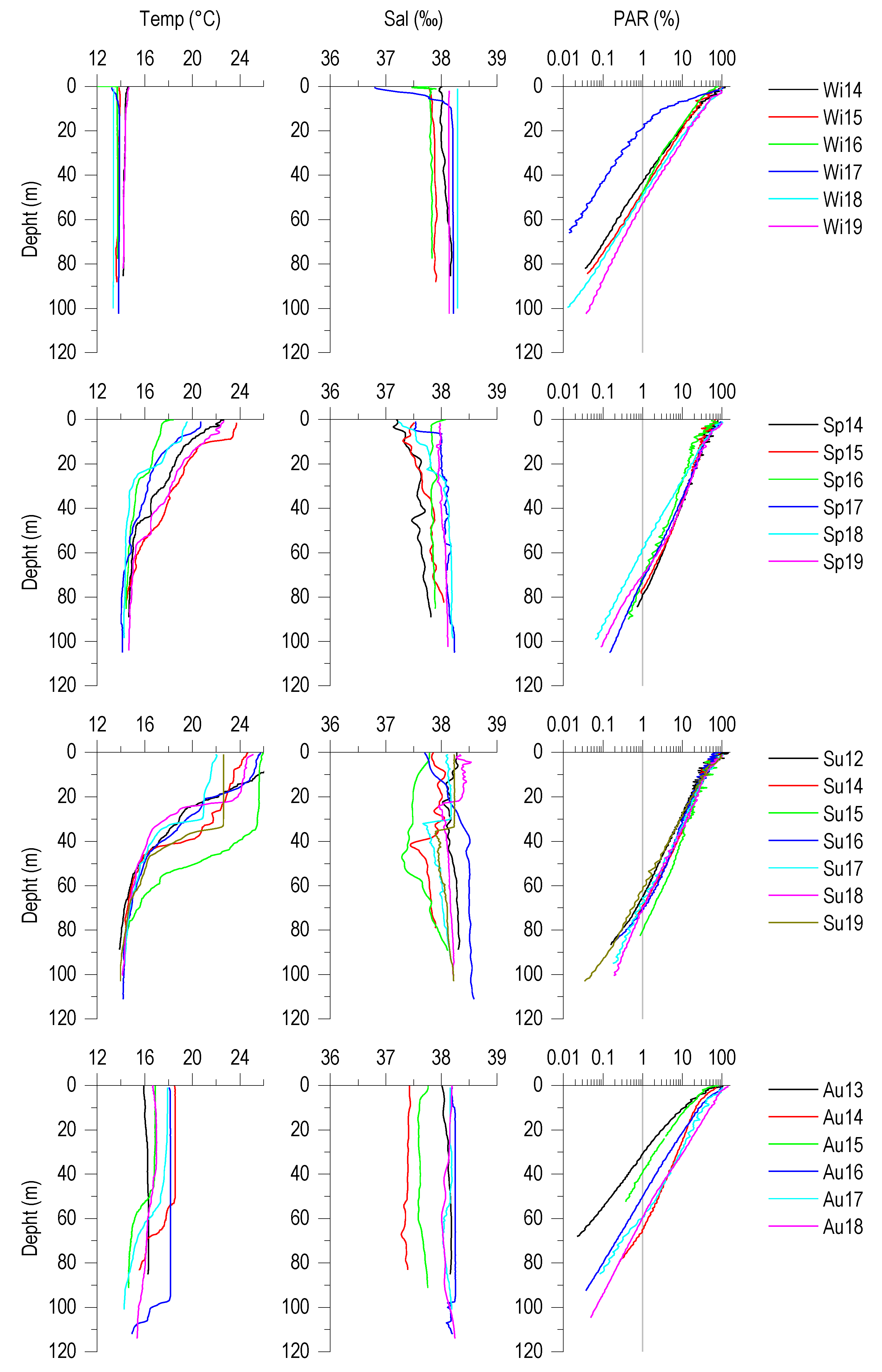
3.1. Vertical Profiles of Temperature, Salinity and PAR (%)

In order to understand CDOM distribution, origin, dynamics, and optical characteristics a preliminary overview on the water vertical structure is necessary (Figure 2). Seasonal modifications are evident mainly at the surface layer as an effect of the atmospheric forcing (cooling/heating) associated to waters mixing processes. During the winter, a homogeneous layer can be observed along the water column. In some case surface salinity low values (near 37‰) were detected as a consequence of strong freshwater discharge. These conditions can sporadically occur in winter and spring. During the spring the formation of an upper mixed layer (UML) less dense than in winter occurred, extended to the first 10–20 m. This stratification condition gained its maximum density differentiation in summer with the deepening of the UML to 30–35 m and a low-density surface water. With a progressive backward path to UML, less differentiated density and deepening occurred towards autumn until returning to the typical winter condition.

PAR (%) profiles indicate the PAR attenuation modalities as a function of depth (Figure 2); from these profiles z_eu can be derived. z_eu were lower and variable in winter and autumn (from less than 20 to 70 m) and were, always in winter and mostly in autumn, in the mixed surface layer. In spring and summer, z_eu were between 70 and 85 m and were always much deeper than the thermocline.

3.2. Zeu/Chl Relationship

An important aspect regarding environmental conditions is represented by the relationship between z_eu and the mean concentration of Chl in the same layer (Figure 3). According to [46], the waters covered by this study can be classified as Case 1 waters in which, following the definition, the main optically active component was phytoplankton. The other optically active substances (CDOM and non-algal particles) are less important and therefore appear in (more or less) constant ratios compared to phytoplankton biomass.

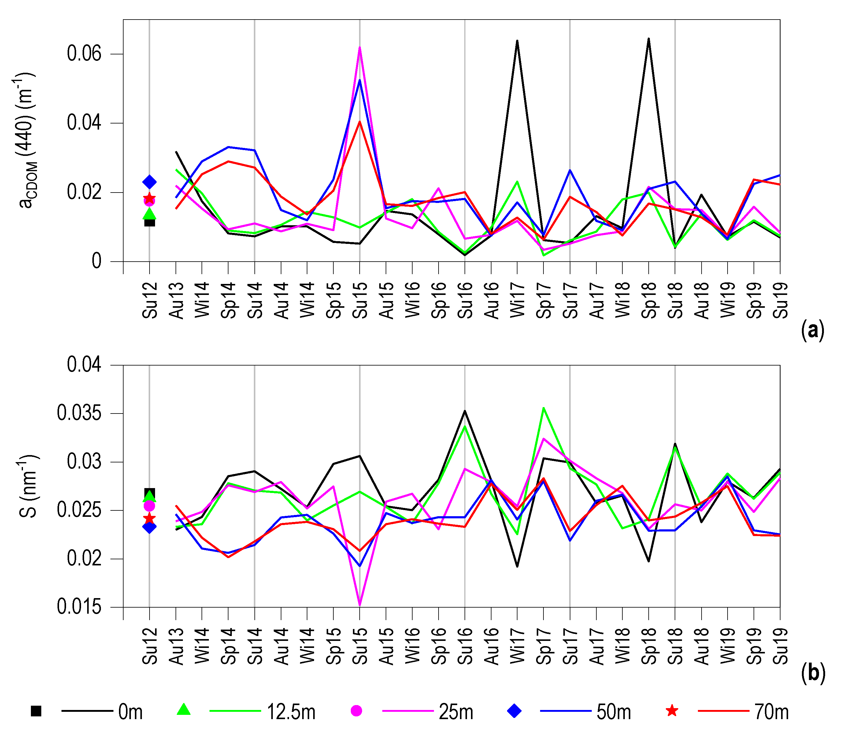
3.3. CDOM Seasonal Evolution

Seasonal and interannual variability of a_CDOM (440) (Figure 4a) and S (Figure 4b), in the surface and the deeper layer were clearly discordant. In the superficial layers a_CDOM (440) maxima (Figure 4a) generally occurred in winter (e.g., Wi17), spring (e.g., Sp18), and autumn (Au13, Au18). In Wi17 and Sp18, the highest values occurred at 0.5 m. These were episodes of strong flooding of the Arno river, following heavy rainfall events and confirmed by direct observation of the weather events and the conditions of the river. On the contrary, all the summer samples show surface minima (Figure 4a), while in the deeper layers, a_CDOM (440) generally had summer maxima, with the highest values generally at 50 m. The coefficient S (Figure 4b) showed an opposite trend. On surface layers (Figure 4b), maxima were in summer (up to 0.036 nm⁻¹) and minima in winter (up to 0.019 nm⁻¹), while in deep layers (Figure 4b), minima were generally in summer.

In summary (

Table 1. Full data and seasonal mean values of a_CDOM (440) (m⁻¹), S (nm⁻¹) and Chl (mg m⁻³) in the entire water column (0.5–70 m), the surface layer (0–25 m) and the deep layer (50–70 m). N: number of samples.

Full Data Set	N	aCDOM (440)	S	Chl
mean	120	0.0154	0.0257	0.2565
standard error	-	0.001	0.0003	0.0242
min	-	0.0018	0.0192	0.0298
max	-	0.0645	0.0356	2.5134
(0.5–70 m)
winter	30	0.0154	0.0249	0.4660
spring	30	0.016	0.0258	0.1652
summer	30	0.016	0.0263	0.1231
autumn	30	0.014	0.0258	0.2696
(0.5–25 m)
winter	18	0.0184	0.0245	0.5379
spring	18	0.0138	0.0271	0.1136
summer	18	0.0067	0.0297	0.0897
autumn	18	0.0141	0.026	0.3035
(50–70 m)
winter	12	0.0148	0.0237	0.3483
spring	12	0.0194	0.0238	0.2530
summer	12	0.0259	0.0225	0.1732
autumn	12	0.014	0.0255	0.2187

), seasonal means of a_CDOM (440) in surface and underlying layers show that in summer the lowest surface and the highest deep values occurred, with the latter higher than the winter surface ones. The highest S was in the summer surface, while the lowest was in the summer deep layer.

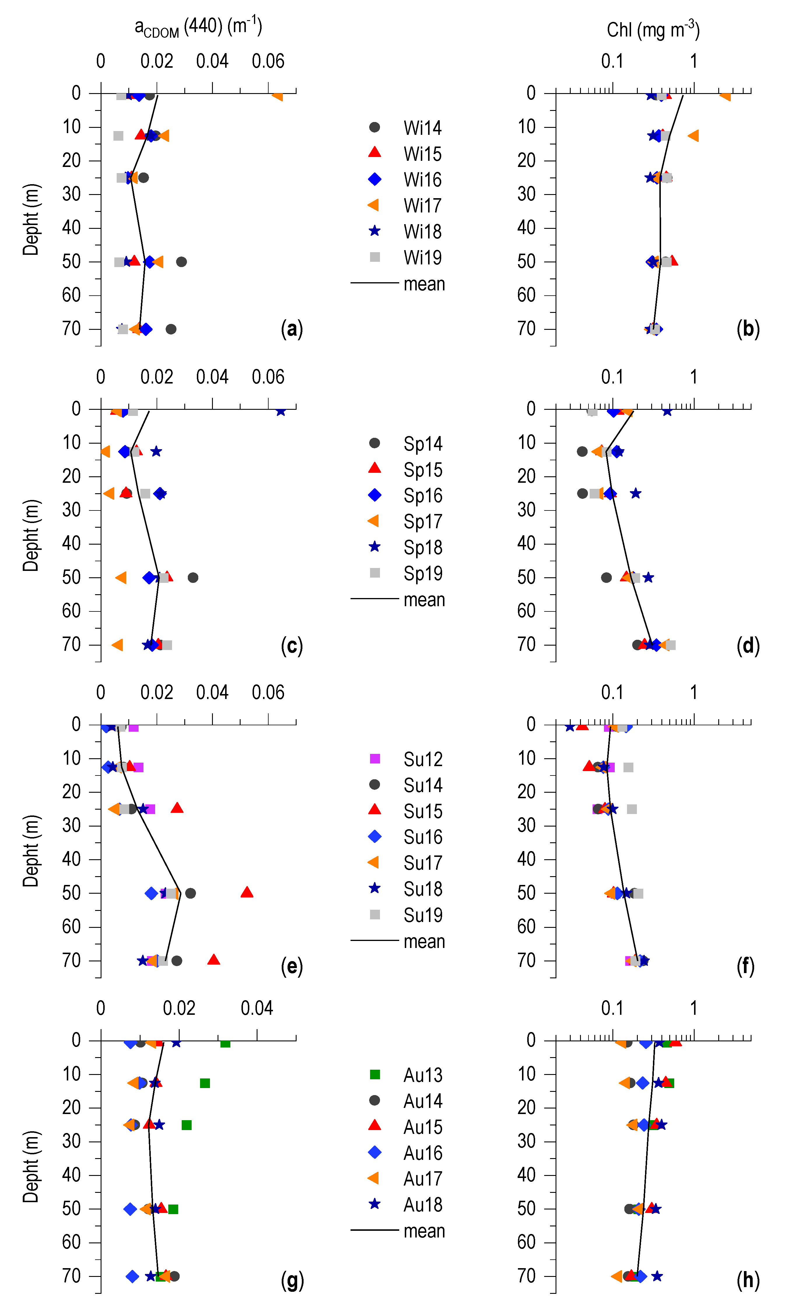
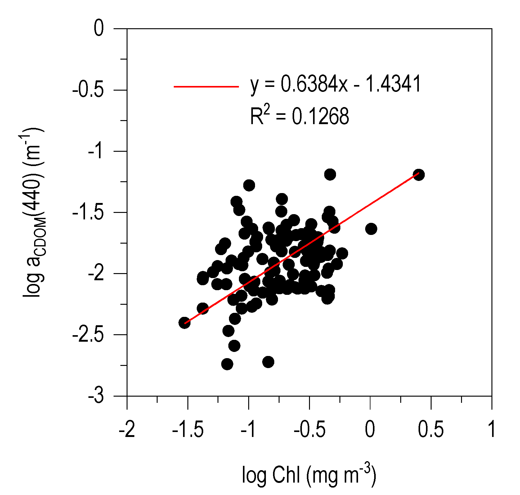
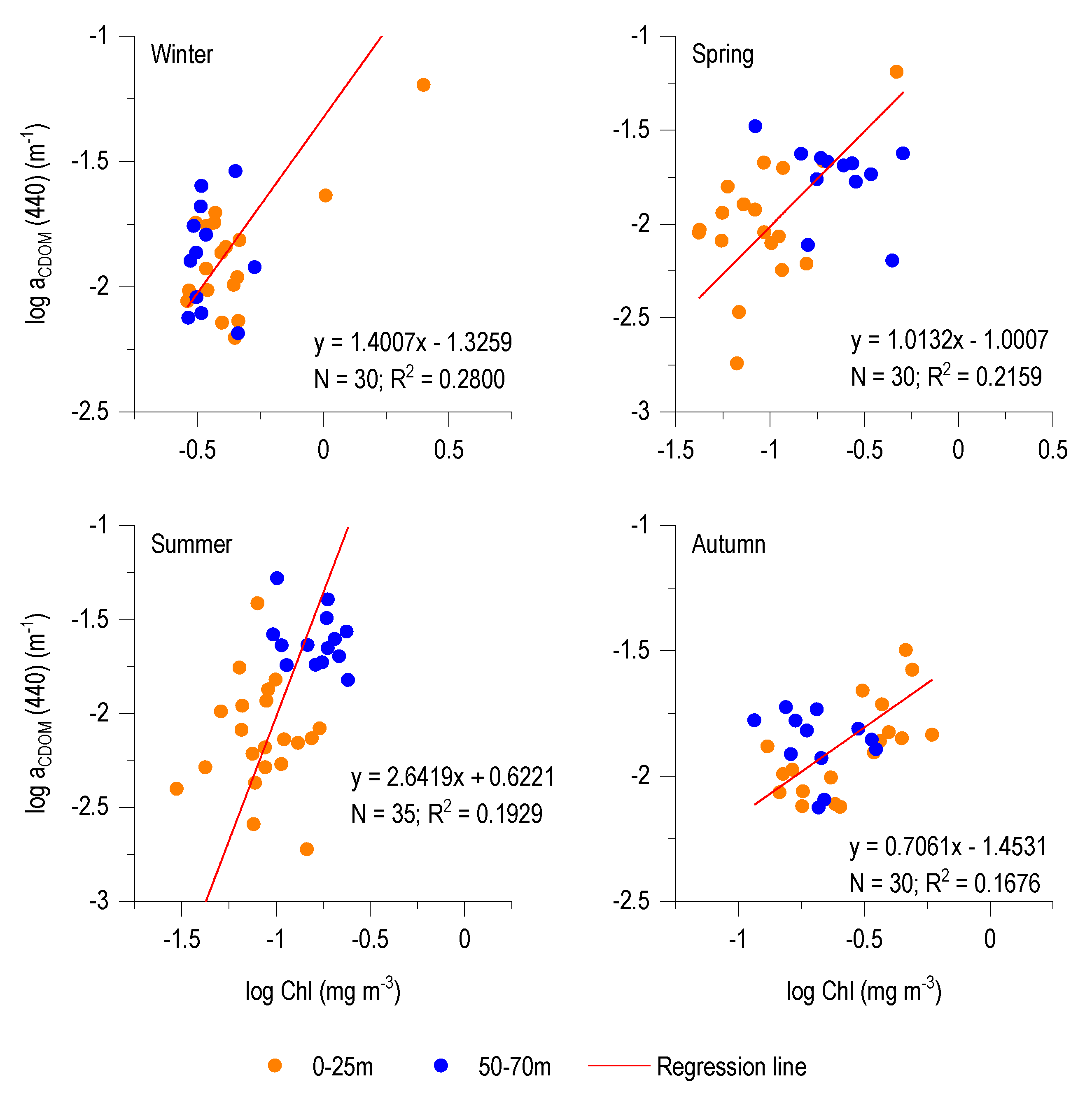
3.4. CDOM-Chl Relationship

The water column structure strongly conditioned the vertical distribution of the a_CDOM (440) and Chl.

In winter a_CDOM (440) distribution along the water column (Figure 5a) was roughly homogenous around 0.015 m⁻¹. Contemporaneously Chl profiles (Figure 5b) showed the annual highest concentration. Profiles are generally characterized by a surface maximum, that in winter 2017 reached the highest value of 2.5 mg m⁻³. From 12.5 to 70 m Chl concentration remains around 0.5 mg m⁻³, with greater variability at 50 m.

In spring a_CDOM (440) mean concentrations and vertical distribution were similar to the winter ones (around 0.016 m⁻¹) (Figure 5c) with a relative maximum at the surface, but the absolute maximum occurred at 50 m. Chl mean concentrations (Figure 5d) were lower respect to winter at all depth excluding 70 m where deep chlorophyll maximum (DCM) occurred. Figure 5a, c also shows that, in Wi17 and Sp18, very high surface a_CDOM (440) occurred. In summer (Figure 5e), the a_CDOM (440) profile shows the greater difference during the year between the two layers: minima at surface and maxima at 50 m. Chl profiles (Figure 5f) generally have lower values at the surface with sub-surface minimum and DCM at 70 m up to 0.3 mg m⁻³. In autumn, a_CDOM (440) (Figure 5g) had generally similar values around 0.014 m⁻¹ from surface to 70 m, with a slight maximum at surface in some cases. Surface Chl concentration (Figure 5h) increased up to 0.4–0.5 mg m⁻³ with respect to the summer values, while remaining similar or lower at 70 m.

Figure 6 summarizes the relationship between a_CDOM (440) and phytoplankton biomass estimated by Chl. This regression has positive correlation coefficient of 0.36 with N = 120 (p < 0.01), and the regression coefficient of about 0.64. Despite the high significance, the points distribution highlights a high variability.

The same relationship, split by seasons (Figure 7), shows greater correlations and high variability of the regression coefficients (from about 0.71 in autumn to 2.6 in summer), highlighting seasonal diversification of processes that bind phytoplankton biomass and CDOM. In winter (Figure 7) the data distribution was fairly homogeneous between the two layers. In the other seasons, especially in spring and in summer, the points belonging to the two different layers can be distinguished. Therefore, the CDOM/Chl ratio varied seasonally and in spring and summer it was different also between the two layers.

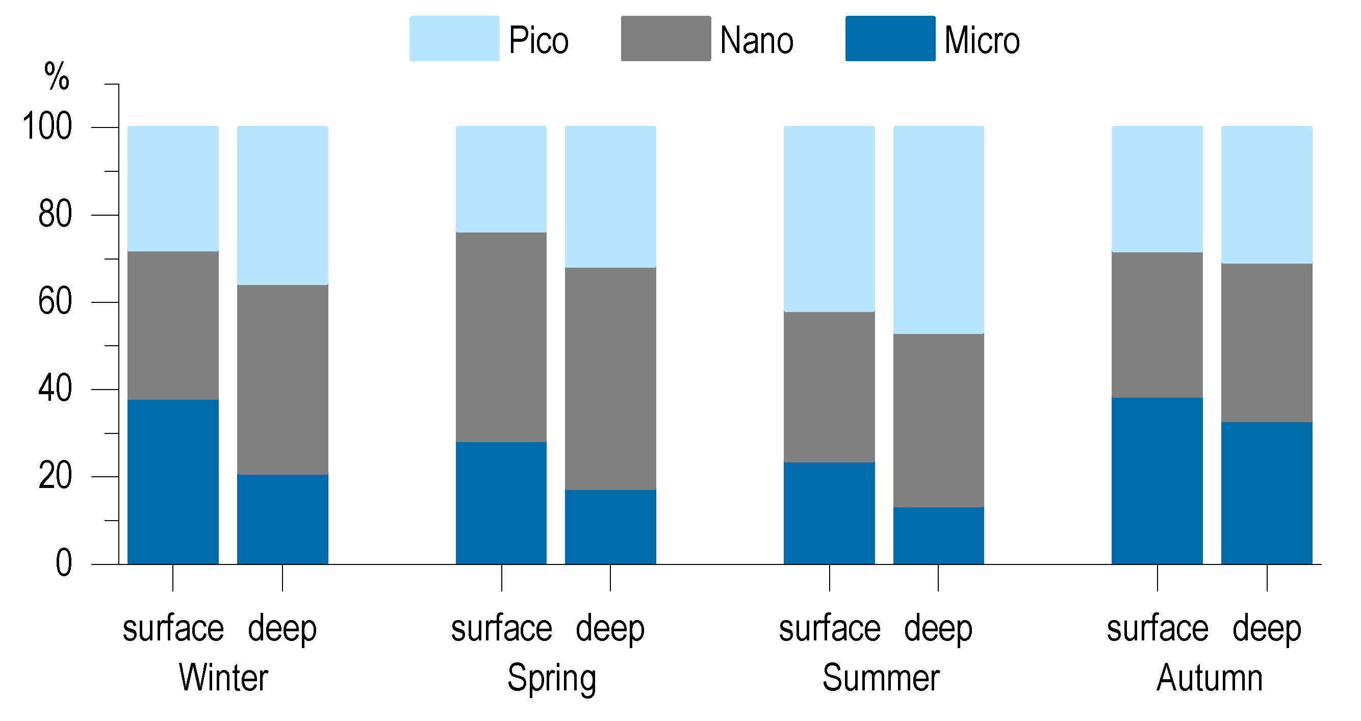
3.5. Phytoplankton Community

Phytoplankton size-fractions contributed in different ways both in seasonal and vertical distribution (Figure 8). Microphytoplankton dominated in winter and autumn surface waters, because of the diatom blooms developed by many taxa. Between them, Cylindrotheca closterium, Plagiotropis cf. lepidoptera, Pseudo-nitzschia spp., and Asterionellopsis glacialis were recurrent in winter, while in autumn, the most abundant were Chaetoceros spp., Cylindrotheca closterium, and Thalassionema frauenfeldii. In spring, nanophytoplankton prevailed with Prymensiophyceae non coccolitophores, represented mainly by the Phaeocystis cf. cordata, observed in the colonial stage too, coccolitophores, and nanoflagellates of different classes. In summer there was a further change in phytoplankton community structure, dominated by picophytoplankton both in surface and in deeper layer albeit with some differences: UML was dominated by cyanobacteria like Synechococcus, and deeper layer by Prochlorococcus, and maybe by picoeukaryotes Chlb containing.

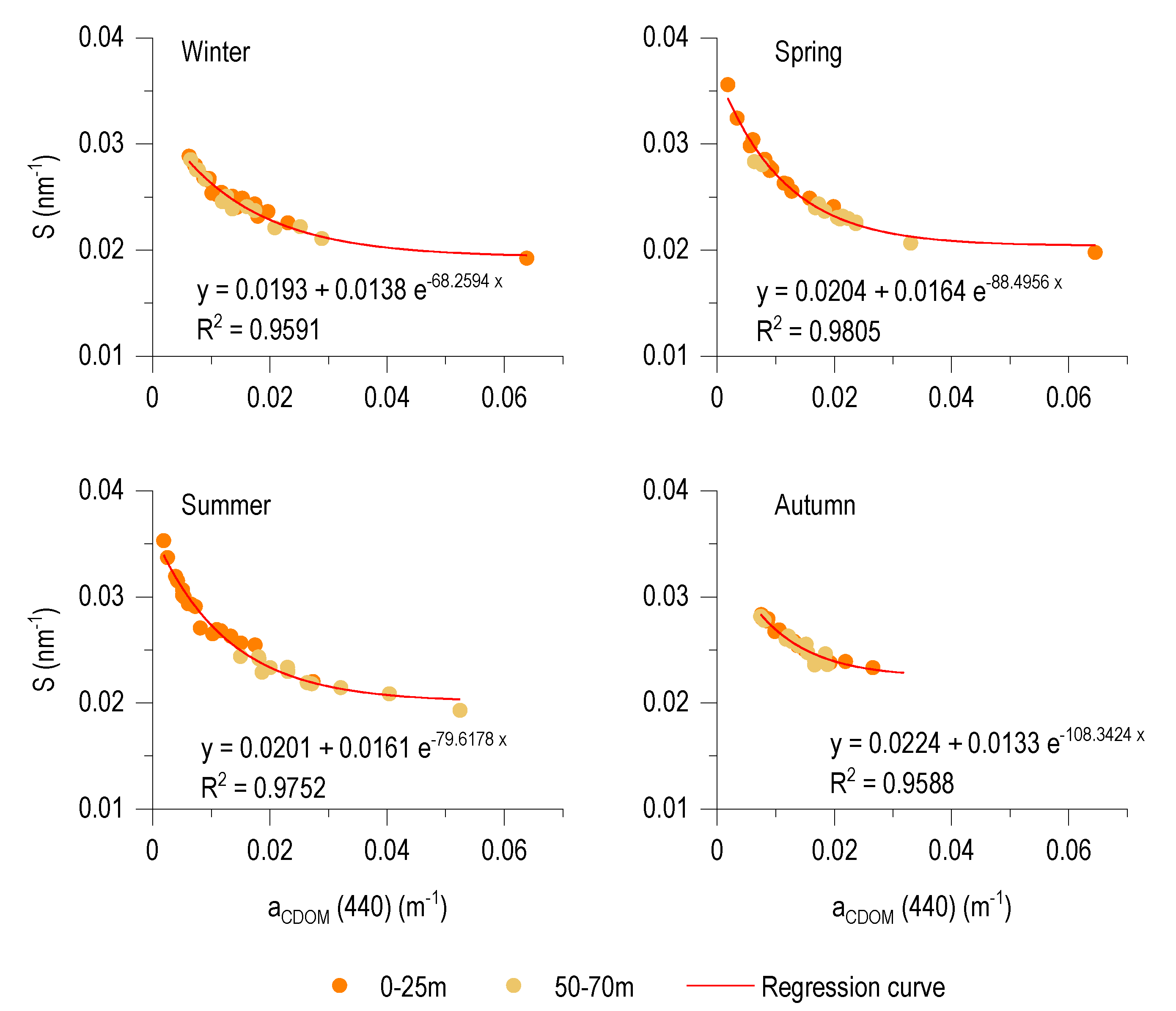
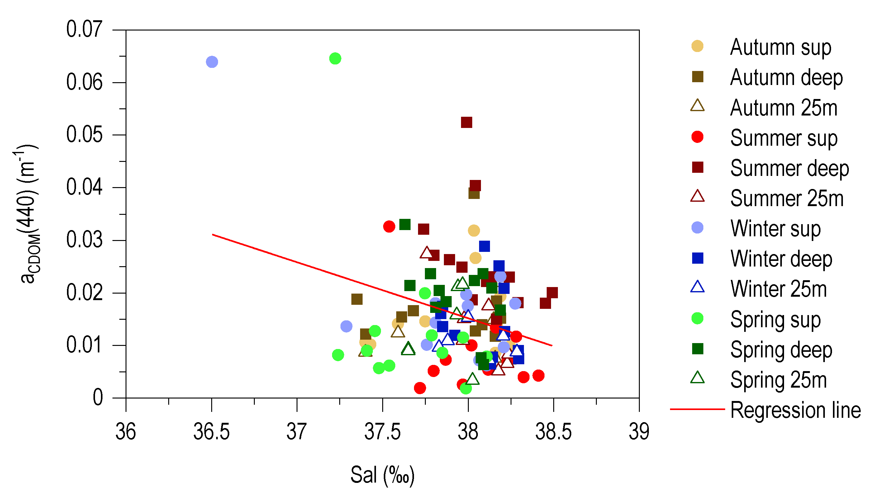
3.6. Relationship between a_CDOM (440) and S

The relationship between a_CDOM (440) and the parameter S that describes the exponential decrease of the CDOM absorption spectrum, has been used, separating the two layers (0–25 m and 50–70 m), to analyze the origin, characteristics and mixing state of the investigated CDOM pools in the different seasons (Figure 9). In winter all samples, regardless of depth, are located rather close with a_CDOM (440) ranging from 0.007 to 0.029 m⁻¹ and S between 0.029 to 0.021 nm⁻¹ with the exception of the Wi17 surface sample that set apart from the other, with a_CDOM (440) approximately 0.064 m⁻¹ and S about 0.019 nm⁻¹.

Similarly, in spring (Figure 9) there was the presence of a single surface sample (Sp18) with high a_CDOM (440) and low S. All the other spring samples had different characteristics than the winter ones: the surface samples were characterized by low a_CDOM (440) and high S while the deep layer had the tendency to place themselves at higher a_CDOM (440) and low S.

In summer, the separation between the surface and deeper samples increased and the trend was inverted: the former showing the lowest annual values of a_CDOM (440) and the highest S while the latter are located at the bottom right of the curve characterized by high a_CDOM (440) and low S. In autumn, sample placement is compacted again in a similar way to winter, with a_CDOM (440) between 0.008 and 0.032 m⁻¹ and S between 0.028 and 0.023 nm⁻¹. The fact that S never falls below 0.023 nm⁻¹ constitutes a distinctive feature of autumn CDOM.

The particular characteristics of both the Wi17 and Sp18 surface samples are further explained by the distribution of a_CDOM (440) vs. salinity (Figure 10). Both the samples are in a clearly separated position from the others and characterized by low salinity values, therefore inputs of fresh waters in the surface layer with high levels of CDOM can be confirmed. Without these two samples, a random distribution of the points emerges and the relationship between a_CDOM (440) vs. salinity completely disappears.

4. Discussion

The data set used in this study was acquired seasonally for about seven years. Clearly, seasonal sampling can represent different conditions due to the annual peculiarities of the weather conditions, but the repetition of the sampling for seven years allows for a sufficiently robust understanding of local conditions.

The mean values of a_CDOM at different wavelengths, S, and other characteristics of the CDOM data set used in this work are reported in

Table 2. Comparison between a_CDOM (λ) (m⁻¹) and S (nm⁻¹) of this study and other data (references in brackets) from Mediterranean Sea. For each S is also showed the non-linear interpolation range.

	This Study				[31]	[28]	[29]	[32]	[34]	[27]
aCDOM (λ)	440	254	300	350	254	300	350	440	254	443
mean	0.0154	1.53	0.48	0.137	1.59		0.103
Standard Error	0.001	0.02	0.01	0.005	0.02		0.003
Min	0.0018	1.13	0.26	0.045		0.08	0.060	0.015	0.69
Max	0.0645	2.54	1.02	0.382		0.58	0.130	0.045	1.54
S	S (250–600)				S (350–400)	S (270–400)	S (350–500)	S (350–500)	S (275–295)	S (350–500)
Mean	0.0257				0.0165	0.0212	0.019			0.017
Standard Error	0.0003				0.0004	0.0004	0.001			0.0038
Min	0.0192						0.014	0.015	0.02	0.0114
Max	0.0356						0.026	0.021	0.04	0.0251

together with recently published CDOM data from various coastal and offshore areas of the Mediterranean Sea. Methodological reasons (different interpolation range and reference wavelengths), local peculiarities, season of sampling, and depth differences make difficult the comparison of the data set, mostly for the Mediterranean waters that show great variability in CDOM concentrations [27]. Despite this, the a_CDOM mean values of this study are very similar to those of the Bay of Marseille [29], the Bay of Blanes [31], and the Boussole site [32] and higher than those of Ionian Sea [28] and those reported by [34]. The mean of S coefficient is 0.0257 nm⁻¹, the highest of the data showed in Table 2, that cover the range between 0.0165 nm⁻¹ [28] and 0.0212 nm⁻¹ [34]. This result could be explained by the interpolation interval used in this work that was extended in the widest possible range [1] to avoid the interference of the finer spectral structures not belonging to CDOM, such as phaeopigments [47], porphyrin [48], and micosporine-like amino acids (MAAs). The choice of this method of interpolation aimed to improve the data interpretation and obtain a more robust estimate of the coefficients a_CDOM (440) and S. The obtained results support the proposed intent in light of the highly significance of the determination coefficients (r²) of the absorption spectra interpolation and of the regression between S vs. a_CDOM (440) always higher than 0.95. Therefore, care must be taken when comparing S values calculated over different wavelength ranges.

4.1. Seasonal Dynamic of CDOM

The seasonal dynamic of the water column structure refers only to epipelagic layer (0–100 m) and is very similar to those of other Mediterranean sites [49,50]. This dynamic is fundamental for understanding the CDOM one.

Typical winter mixed conditions favored an almost homogeneous vertical distribution of a_CDOM (440). In spring, surface a_CDOM (440) was generally lower than in winter with higher S values, while below the UML, which in the meantime is forming, a_CDOM (440) showed an increase, compared to the winter ones, and a decrease of S. Therefore, starting from a single winter CDOM pool, the tendency to form two pools, one in the UML and the other near the DCM, followed the modification of the water column structure.

The increase in solar irradiance and UV from spring to summer, involves CDOM photobleaching process in the UML. As a consequence, the summer surface samples were characterized by the lowest a_CDOM (440) mean value and highest S. Below UML, instead, the highest a_CDOM (440) mean values with low S were reached. In autumn, the two summer pools tend to mix thanks to the weakening of thermocline and halocline and to the disappearance of stratification, so the CDOM pool present in the water column had similar characteristics.

During the seven years of the survey mean seasonal maxima concentration of CDOM (excluding the two terrigenous input events) were recorded in summer in the 50–70 m layer (a_CDOM (440) 0.0259 m⁻¹ and S 0.0225 nm⁻¹) contemporaneously to the presence of the DCM. In this layer a_CDOM (440) mean increased of about 40% if compared to winter one. A similar increase was reported by [12] for the Middle Atlantic Bight.

The summarized CDOM dynamic is similar to those previously described at the Bermuda Atlantic Time-Series [13,14] and similar to both dynamic and average concentrations for other Western Mediterranean Sea areas as at Boussole site [32], in front of the Marseille Bay [29] and near of the Blanes Bay [31].

The high a_CDOM (440) in the surface layer in winter is known for Mediterranean and described by many authors both with direct measurements [28,29,30,31,32,34], by remote sensing [18,51] or derived from measurements with Bio-Argo Floats [52,53]. Morel and Gentili [18] related the presence of high CDOM concentration in winter surface waters to the nature of the semi enclosed Mediterranean basin influenced by the increased winter-spring rivers flows.

The position of the site here analyzed, located on the continental shelf, about 23 km from the coast, south of the Arno river estuary may suggest a possible strong influence of freshwater inputs on the concentrations of CDOM. From the relationship between salinity and a_CDOM (440) the site did not appear to behave as a typical coastal area where the supply of freshwaters rich in CDOM is always significant in time as reported for many areas [54,55,56,57,58]. The study site in normal conditions or even with an increased flow rate, is not directly affected by freshwaters with high CDOM concentration [59,60] because a_CDOM (440) values appear similar to other Western Mediterranean offshore areas. Only with exceptional flood these waters can directly affect the area and significantly change the levels of CDOM, as happened in winter 2017 and spring 2018, when surface waters were clearly affected by freshwater runoff and terrigenous inputs. During these events surface a_CDOM (440) reached the highest level and S the lowest. The results obtained show that these events are only sporadic and focused on specific conditions that can occur in the periods of greatest rainfall such as winter, spring, or autumn.

The summer superficial pool of CDOM was characterized by the strong decrease of a_CDOM (440) to the annual minimum, together with an increase of S up to the highest values. The condition of low a_CDOM (440) associated with high S is common in other areas of the Mediterranean Sea [28,29,31,32,34] and in other intermediate and tropical latitudes, particularly for Atlantic Ocean [13,61], as a consequence of the photobleaching process of CDOM driven by absorption of UV band. Consequently, a fraction of Carbon escapes in atmosphere as CO₂, altering the spectral properties of CDOM for the loss in absorption by the chromophore [62,63,64]. From winter to summer, a significant loss of CDOM concentration occurs every year in UML as a_CDOM (440) was found to decrease on average by about 60%, and in some years, as in 2017, the decrease can exceed 80%. This means that a large part of winter CDOM production was removed via photobleaching. Many authors [12,13,65,66,67] confirmed CDOM photobleaching as the most important sinking process for CDOM and one of the contributions to take into account in the frame of global warming.

4.2. a_CDOM (440)–Chl Relationship

Focusing on biological activity, CDOM can be produced by several direct (e.g., extracellular release and excretion, sloppy feeding, cell lysis) or indirect (zooplankton feeding and bacterial degradation of dead cells and debris) phytoplanktonic processes [16].

The above mentioned analysis of CDOM dynamic in the Ligurian site, show how its maxima, both during the surface winter bloom and in the summer 50–70 m layer of DCM, are always associated with phytoplankton biomass maxima (absolute or relative), as confirmed by the general regression between a_CDOM (440) and Chl. A first quantitative estimate for surface waters was obtained by [18] using a power model: a_CDOM (443) = 0.0316 Chl^0.63, confirmed, with small changes, by [47] and by [32] notwithstanding the high variability in data distribution. Likewise, in the present study, despite the high significance of the correlation coefficient (p < 0.01) and the very similar regression coefficient (0.638) a high variability can be pointed out. The same regression studied by [13,19] provided similar data dispersion, while [28] used a linear model, obtaining a high correlation.

If the relationship a_CDOM (440) vs. Chl is splitted for each season, still keeping positive trend, multiple quantitative modalities emerge. Even if organic matter in the open sea is mainly due to phytoplanktonic primary production, their linkage can be direct or largely indirect, mediated by the activity of other organisms at different time scales and modified by physical phenomena such as surface photobleaching or the sporadic terrigenous influx.

The quantitative relationship between phytoplankton biomass and CDOM, in addition to its ecological value, has considerable importance for practical purposes in relation to satellite Chl estimates [68] especially in the Mediterranean Sea [18,24,30].

The results of this work highlight the complexity of the link between phytoplankton biomass and CDOM, involving different phases of the Carbon cycle, leading to the need of local studies and data acquisition to improve the Mediterranean satellite estimate of Chl.

4.3. Spectral Characteristics and Origin of CDOM

According to [28,44], CDOM optical characteristics have been analyzed on the basis of the relationship between a_CDOM (440) and S. S is not influenced by CDOM concentration, but a_CDOM (440) and S are strictly linked to its composition and also to its origin. a_CDOM (440) and S are specific characteristics of different pools of CDOM, each of these characterized by specific values. In the present study, the pools (end point) that can be clearly distinguished are:

(1)

The surface one linked to terrestrial input events.

(2)

The surface summer one, with low absorption and high S.

(3)

The winter entire water column one.

(4)

The deep summer layer one characterized by high a_CDOM (440) and low S.

The CDOM pools present in spring and autumn on the surface or in the deep layer, due to their characteristics, appear as phases of transition (formation of UML and its disappearance) towards the last three most consolidated extreme conditions. Apart from the above-mentioned first pool of terrestrial origin the surface summer pool can be recognized according to its spectral characteristics (very low a_CDOM (440) and very high S) and it originated from the photobleaching [64,69].

The other two pools identified, the winter and the deep layer summer ones, had high a_CDOM (440) (summer ones are greater than winter ones) and low S (deep summer ones are lower than winter ones), both associated with Chl maxima, higher in winter than in the DCM.

If in winter a more direct link between phytoplankton production and CDOM appears, CDOM summer pool usually was mostly concentrated immediately above the maximum of Chl, showing an example of an indirect relationship between CDOM and Chl. Summer DCM and a_CDOM(440) maxima were always out of phase: DCM was always at 70 m, while the CDOM maxima at 50 m. Many other authors have described similar structure [13,19,32,34,70]. Organelli et al. [32] noted similarities between the vertical distribution of bacterioplankton and CDOM at the Boussole site, their maxima were at the same depth over DCM, assuming in these conditions a preponderant role of bacterioplankton in the production of CDOM.

Regarding the phytoplankton composition, a strong seasonal change is evident, from microphytoplankton in winter to picoplankton in summer passing through nanophytoplankton dominance in spring. Taxonomic structure of phytoplankton community is an indicator of the marine ecosystem, trophic and biogeochemical states [71,72,73,74,75]. Diatoms, that dominate the winter assemblage, are known to have a high efficiency in transferring organic substance to the upper levels of the trophic network [76]. Then, once bloom is exhausted due to grazing and nutrient depletion in the new formed UML, microphytoplankton biomass is in part immediately decomposed and in part settles as organic particles that can sediment in the underlying layer, contributing to CDOM production. An aspect to highlight is the detection of Phaeocystis cf. cordata in spring, mainly at 50 m, in the colonial form embedded in the mucous matrix. For some species of the same genus (Phaeocystis antarctica) a close link with the production of CDOM has been highlighted [77]. Therefore, the presence of colonies could represent one of the indirect links, out of time, between phytoplankton and CDOM mediated by bacteria, but at the moment it can only constitutes a further working hypothesis to be explored to understand its quantitative importance.

The summer dominant picoplankton fraction instead, is generally associated with a different trophic network supported mainly by debris and characteristic of oligotrophic conditions. For this condition, [78] developed the concept of “microbial loop” to indicate a trophic web sustained by the recycling of the organic matter produced by picophytoplankton and in which bacteria play a fundamental role. DOC excretion rates are constrained by abundance and taxonomic composition of primary producers in the ecosystem. Smaller phytoplankton have been shown to excrete a higher percentage of their assimilated carbon as DOC than their larger counterparts [79,80,81]. This great excretion of DOC can have potentially large impacts on food webs and may change the ecosystem dynamics toward microbial loop. The occurrence of these processes affects CDOM production both directly from phytoplankton or indirectly from bacterial utilization and transformation of DOM labile fraction, excreted by phytoplankton. CDOM is a less labile form of dissolved organic substance which therefore can also accumulate. This hypothesis seems to be in agreement with the results of other authors who, in similar conditions, associate the maximum of CDOM with the maximum of the vertical distribution of the bacterioplankton [32,70].

So, the two recognized pools of high CDOM concentration, characterized by different S, have been identified in two completely different trophic regimes and, particularly, with two different phytoplanktonic communities: microphytoplankton dominated by diatoms on the surface in winter and picophytoplankton in the summer deep layer.

4.4. Implications for Remote Sensing

From the recognized CDOM dynamic it is clear that its optical properties (a_CDOM (440) and S) vary considerably over the year as well as the relationships between phytoplankton biomass and a_CDOM (440). These two aspects are fundamental for remote sensing applications. Reference [18] highlights as a critical aspect of the functioning of standard algorithms for estimation of Chl in Mediterranean Sea that the estimate errors vary during the year and are greater in winter and much smaller in summer. These characteristics, based on the results of this study, can be interpreted as consequent to the seasonal variations of the optical properties of CDOM and CDOM/Chl ratios.

Therefore, the Mediterranean regional algorithms to estimate CDOM and Chl should take into account these seasonal trends considering both CDOM optical properties, particularly S, and Chl/CDOM as seasonal variables. These implementations could be crucial to improve the current estimates in the Mediterranean Sea, which have the most critical aspect in the CDOM component, as emphasized by many authors [18,24,30,82].

5. Conclusions

The dynamic of CDOM in the photic zone of the Mediterranean shelf waters examined is determined by the interaction of biological, physico-chemical, and hydrodynamical processes.

Biological processes are certainly prevalent in CDOM production and modification (especially in surface winter spring and in summer deep layer) and coupled with thermohaline seasonal variations accounts for the main features of CDOM distribution on the water column. The spring–summer UML formation and consolidation cause strong sink of CDOM due to photobleaching.

Only strong flooding events can directly influence surface water of the sampling site determining very high supply of terrigenous CDOM.

Even in continental shelf site such as that considered in this study CDOM production is essentially linked to autochthonous biological processes in which phytoplankton is the main agent both through direct production and degradation of its biomass. Despite this, the relationship between CDOM and Chl has high variability due to the different ways in which CDOM is linked to phytoplankton. Chl, consequently cannot be considered a robust proxi of CDOM even in Case 1 waters such as those investigated.

During the years of investigation, CDOM production processes and consequent accumulation occur essentially during the winter bloom in the surface layer and during the deep summer maxima of Chl (DCM). In both cases the CDOM pools are characterized by high a_CDOM (440) and low S but each with its own peculiarities which allow to distinguish them. They originated in very different ecological and trophic conditions characterized by the dominance of diatoms in winter, and picophytoplankton in summer deep layer with the bacterial component that most likely plays a very important role.

The described dynamics lead to strong differences in a_CDOM (440) along the year which, depending on the layer and year, can vary from 50% to 80%.

The results of this work highlight the strong dynamism of CDOM and its multiple implications in the functioning of the photic zone of marine ecosystem and confirm the complexity of the link between phytoplankton biomass and CDOM, involving different phases of the Carbon cycle. Moreover, these results suggest some important inputs to be introduced for the improvement of the Mediterranean satellite estimates of Chl and CDOM, such as the seasonal differentiation of the optical properties, particularly S, and the relationships between Chl and CDOM.

References

1. Blough, N.V.; Del Vecchio, R. Chromophoric DOM in the Coastal Environment. In Biogeochemistry of Marine Dissolved Organic Matter; Hansell, D.A., Carlson, C.A., Eds.; Academic Press: San Diego, CA, USA, 2002; pp. 509–546. [Google Scholar] [CrossRef]
2. Thurman, E.M. Aquatic Humic Substances. In Organic Geochemistry of Natural Waters. Developments in Biogeochemistry; Springer: Dordrecht, The Netherlands, 1985; Volume 2, pp. 273–361. [Google Scholar] [CrossRef]
3. Mopper, K.; Kieber, D.J. Photochemistry and the Cycling of Carbon, Sulfur, Nitrogen and Phosphorus. In Biogeochemistry of Marine Dissolved Organic Matter; Hansell, D.A., Carlson, C.A., Eds.; Academic Press: San Diego, CA, USA, 2002; pp. 455–507. [Google Scholar] [CrossRef]
4. Bushaw, K.L.; Zepp, R.G.; Tarr, M.A.; Shulz-Jander, D.; Bourbonniere, R.A.; Hodson, R.E.; Miller, W.L.; Bronk, D.A.; Moran, M.A. Photochemical release of biologically available nitrogen from aquatic dissolved organic matter. Nature 1996, 381, 404–407. [Google Scholar] [CrossRef]
5. Miller, W.L. Effects of UV Radiation on Aquatic Humus: Photochemical Principles and Experimental Considerations. In Aquatic Humic Substances. Ecological Studies (Analysis and Synthesis); Hessen, D.O., Tranvik, L.J., Eds.; Springer: Berlin/Heidelberg, Germany, 1998; Volume 133, pp. 125–126. [Google Scholar]
6. Wrigley, T.J.; Chambers, J.M.; McComb, A.J. Nutrient and gilvin levels in waters of coastal-plain wetlands in an agricultural area of Western Australia. Mar. Freshwater Res. 1988, 39, 685–694. [Google Scholar] [CrossRef]
7. Davies-Colley, R.J. Yellow substance in coastal and marine waters around the South Island, New Zealand. N. Z. J. Mar. Fresh. 1992, 26, 311–322. [Google Scholar] [CrossRef] [Green Version]
8. Carder, K.L.; Hawes, S.K.; Baker, K.A.; Smith, R.C.; Steward, R.G.; Mitchell, B.G. Reflectance model for quantifying chlorophyll a in the presence of productivity degradation products. J. Geophys. Res. 1991, 96, 20599–20611. [Google Scholar] [CrossRef] [Green Version]
9. Carder, K.L.; Chen, F.R.; Lee, Z.P.; Hawes, S.K.; Kamykowski, D. Semianalytic Moderate-resolution imaging spectrometer algorithms for chlorophyll A and absorption with bio-optical domains based on nitrate-depletion temperatures. J. Geophys. Res. 1999, 104, 5403–5421. [Google Scholar] [CrossRef]
10. Kalle, K. Zum Problem des Meercswasserfarbc. Ann. Hydrol. Mar. Mitt. 1938, 66, 1–13. [Google Scholar]
11. Jerlov, N.G. Influence of suspended and dissolved matter on the transparency of sea water. Tellus 1953, 5, 59–65. [Google Scholar] [CrossRef]
12. Vodacek, A.; Blough, N.V.; DeGrandpre, M.D.; Peltzer, E.T.; Nelson, R.K. Seasonal variation in CDOM and DOC in the Middle Atlantic Bight: Terrestrial inputs and photo-oxidation. Limnol. Oceanogr. 1997, 42, 674–768. [Google Scholar] [CrossRef] [Green Version]
13. Nelson, N.B.; Siegel, D.A.; Michaels, A.F. Seasonal dynamics of colored dissolved material in the Sargasso Sea. Deep Sea Res. Part I 1998, 45, 931–957. [Google Scholar] [CrossRef]
14. Nelson, N.B.; Siegel, D.A. Chromophoric DOM in the Open Ocean. In Biogeochemistry of Marine Dissolved Organic Matter; Hansell, D.A., Carlson, C.A., Eds.; Academic Press: San Diego, CA, USA, 2002; pp. 547–578. [Google Scholar] [CrossRef]
15. Nelson, N.B.; Siegel, D.A. The global distribution and dynamics of chromophoric dissolved organic matter. Annu. Rev. Mar. Sci. 2013, 5, 447–476. [Google Scholar] [CrossRef] [Green Version]
16. Coble, P.G. Marine optical biogeochemistry: The chemistry of ocean color. Chem. Rev. 2007, 107, 402–418. [Google Scholar] [CrossRef] [PubMed]
17. DeGrandpre, M.D.; Vodacek, A.; Nelson, R.K.; Bruce, E.J.; Blough, N.V. Seasonal seawater optical properties of the U.S. Middle Atlantic Bight. J. Geophys. Res. 1996, 101, 22727–22736. [Google Scholar] [CrossRef]
18. Morel, A.; Gentili, B. The dissolved yellow substance and the shades of blue in the Mediterranean Sea. Biogeosciences 2009, 6, 2625–2636. [Google Scholar] [CrossRef] [Green Version]
19. Kitidis, V.; Stubbins, A.P.; Uher, G.; Upstill Goddard, R.C.; Lawb, C.S.; Woodward, E.M.S. Variability of chromophoric organic matter in surface waters of the Atlantic Ocean. Deep Sea Res. Part II 2006, 53, 1666–1684. [Google Scholar] [CrossRef]
20. Antoine, D.; Morel, A.; André, J.M. Algal pigment distribution and primary production in the Eastern Mediterranean as derived from coastal zone color scanner observations. J. Geophys. Res. 1995, 100, 193–209. [Google Scholar] [CrossRef]
21. Bricaud, A.; Bosc, E.; Antoine, D. Algal biomass and sea surface temperature in the Mediterranean Basin: Intercomparison of data from various satellite sensors, and implications for primary production estimates. Remote Sens. Environ. 2002, 81, 163–178. [Google Scholar] [CrossRef]
22. Volpe, G.; Santoleri, R.; Vellucci, V.; Ribera d’Alcalà, M.; Marullo, S.; D’Ortenzio, F. The colour of the Mediterranean Sea: Global versus regional bio-optical algorithms evaluation and implication for satellite chlorophyll estimates. Remote Sens. Environ. 2007, 107, 625–638. [Google Scholar] [CrossRef]
23. Antoine, D.; D’Ortenzio, F.; Hooker, S.B.; Bécu, G.; Gentili, B.; Tailliez, D.; Scott, A.J. Assessment of uncertainty in the ocean reflectance determined by three satellite ocean color sensors (MERIS, SeaWiFS and MODIS-A) at an offshore site in the Mediterranean Sea (BOUSSOLE project). J. Geophys. Res. 2008, 113. [Google Scholar] [CrossRef]
24. Lapucci, C.; Rella, M.A.; Brandini, C.; Ganzin, N.; Gozzini, B.; Maselli, F.; Massi, L.; Nuccio, C.; Ortolani, A.; Trees, C. Evaluation of empirical and semi-analytical chlorophyll algorithms in the Ligurian and North Tyrrhenian Seas. J. Appl. Remote Sens. 2012, 6. [Google Scholar] [CrossRef] [Green Version]
25. Xing, X.; Morel, A.; Claustre, H.; D’Ortenzio, F.; Poteau, A. Combined processing and mutual interpretation of radiometry and fluorometry from autonomous profiling Bio-Argo floats: 2. Colored dissolved organic matter absorption retrieval. J. Geophys. Res. 2012, 117, C04022. [Google Scholar] [CrossRef] [Green Version]
26. Lee, Z.; Hu, C. Global distribution of Case-1 waters: An analysis from SeaWiFS measurements. Remote Sens. Environ. 2006, 101, 270–276. [Google Scholar] [CrossRef]
27. Babin, M.; Stramski, D.; Ferrari, G.M.; Claustre, H.; Bricaud, A.; Obolensky, G.; Hoepffner, N. Variations in the light absorption coefficients of phytoplankton, nonalgal particles, and dissolved organic matter in coastal waters around Europe. J. Geophys. Res. 2003, 108, 3211. [Google Scholar] [CrossRef]
28. Bracchini, L.; Tognazzi, A.; Dattilo, A.M.; Decembrini, F.; Rossi, C.; Loiselle, S.A. Sensitivity analysis of CDOM spectral slope in artificial and natural samples: An application in the central eastern Mediterranean Basin. Aquat. Sci. 2010, 72, 485–498. [Google Scholar] [CrossRef]
29. Para, J.; Coble, P.G.; Charrière, B.; Tedetti, M.; Fontana, C.; Sempéré, R. Fluorescence and absorption properties of chromophoric dissolved organic matter (CDOM) in coastal surface waters of the Northwestern Mediterranean Sea (Bay of Marseilles, France). Biogeosciences 2010, 7, 4083–4103. [Google Scholar] [CrossRef] [Green Version]
30. Massi, L.; Santini, C.; Pieri, M.; Nuccio, C.; Maselli, F. Use of MODIS imagery for the optical characterization of Western Mediterranean water. Ital. J. Remote Sens. 2011, 43, 19–37. [Google Scholar] [CrossRef]
31. Romera-Castillo, C.; Álvarez-Salgado, X.A.; Galí, M.; Gasol, J.M.; Marrasé, C. Combined effect of light exposure and microbial activity on distinct dissolved organic matter pools. A seasonal field study in an oligotrophic coastal system (Blanes Bay, NW Mediterranean). Mar. Chem. 2013, 148, 44–51. [Google Scholar] [CrossRef] [Green Version]
32. Organelli, E.; Bricaud, A.; Antoine, D.; Matsuoka, A. Seasonal dynamics of light absorption by chromophoric dissolved organic matter (CDOM) in the NW Mediterranean Sea (BOUSSOLE site). Deep Sea Res. Part I 2014, 91, 72–85. [Google Scholar] [CrossRef]
33. Santinelli, C. DOC in the Mediterranean Sea. In Biogeochemistry of Marine Dissolved Organic Matter, 2nd ed.; Hansell, D.A., Carlson, C.A., Eds.; Academic Press: San Diego, CA, USA, 2015; pp. 579–608. [Google Scholar] [CrossRef]
34. Galletti, Y.; Gonnelli, M.; Retelletti Brogi, S.; Vestri, S.; Santinelli, C. DOM dynamics in open waters of the Mediterranean Sea: New insights from optical properties. Deep. Sea Res. I. 2019, 144, 95–114. [Google Scholar] [CrossRef]
35. Vidussi, F.; Claustre, H.; Bustilloz-Guzmàn, J.; Cailliau, C.; Marty, J.C. Rapid HPLC method for determination of phytoplankton chemotaxinomic pigments: Separation of chlorophyll a from divinyl-chlorophyll a and zeaxanthin from lutein. J. Plankton Res. 1996, 18, 2377–2382. [Google Scholar] [CrossRef] [Green Version]
36. Barlow, R.G.; Cummings, D.G.; Gibb, S.W. Improved resolution of mono- and divinyl chlorophylls a and b and zeaxanthin and lutein in phytoplankton extracts using reverse phase C-8 HPLC. Mar. Ecol. Prog. Ser. 1997, 161, 303–307. [Google Scholar] [CrossRef]
37. Bricaud, A.; Claustre, H.; Ras, J.; Oubelkheir, K. Natural variability of phytoplanktonic absorption in oceanic waters: Influence of the size structure of algal populations. J. Geophys. Res. 2004, 109, 1–12. [Google Scholar] [CrossRef]
38. Vidussi, F.; Claustre, H.; Manca, B.; Luchetta, A.; Marty, J. Phytoplankton pigment distribution in relation to upper thermocline circulation in the Eastern Mediterranean Sea during winter. J. Geophys. Res. 2001, 106, 19939–19956. [Google Scholar] [CrossRef]
39. Zingone, A.; Totti, C.; Sarno, D.; Caroppo, C.; Giacobbe, M.G.; Lugliè, A.; Nuccio, C.; Socal, G. Fitoplancton: Metodiche di analisi quali-quantitativa. In Metodologie di Campionamento e di Studio del Plancton Marino; Socal, G., Buttino, I., Cabrini, M., Mangoni, O., Penna, A., Totti, C., Eds.; Manuali e Linee Guida ISPRA-SIBM: Rome, Italy, 2010; Volume 56, pp. 213–237. [Google Scholar]
40. Nayar, S.; Chou, L.M. Relative efficiencies of different filters in retaining phytoplankton for pigment and productivity studies. Estuar. Coast. Shelf. Sci. 2000, 58, 241–248. [Google Scholar] [CrossRef]
41. Ferrari, G. The relationship between chromophoric dissolved organic matter and dissolved organic carbon in the European Atlantic coastal area and in the West Mediterranean Sea (Gulf of Lions). Mar. Chem. 2000, 70, 339–357. [Google Scholar] [CrossRef]
42. Bricaud, A.; Morel, A.; Prieur, L. Absorption by dissolved organic matter of the sea (yellow substance) in the UV and visible domains. Limnol. Oceanogr. 1981, 26, 43–53. [Google Scholar] [CrossRef]
43. Kowalczuk, P.; Cooper, W.J.; Whitehead, R.F.; Durako, M.J.; Sheldon, W. Characterization of CDOM in an organic-rich river and surrounding coastal ocean in the South Atlantic Bight. Aquat. Sci. 2003, 65, 384–401. [Google Scholar] [CrossRef]
44. Stedmon, C.A.; Markager, S. The optics of chromophoric dissolved organic matter (CDOM) in the Greenland Sea: An algorithm for differentiation between marine and terrestrially derived organic matter. Limnol. Oceanogr. 2001, 46, 2087–2093. [Google Scholar] [CrossRef]
45. Twardowski, M.S.; Boss, E.; Sullivan, J.M.; Donaghay, P.L. Modeling the spectral shape of absorption by chromophoric dissolved organic matter. Mar. Chem. 2004, 89, 69–88. [Google Scholar] [CrossRef]
46. Morel, A. Optical modeling of the upper ocean in relation to its biogenous matter content (case 1 water). J. Geophys. Res. 1988, 93, 10749–10768. [Google Scholar] [CrossRef] [Green Version]
47. Bricaud, A.; Babin, M.; Claustre, H.; Ras, J.; Tièche, F. Light absorption properties and absorption budget of Southeast Pacific waters. J. Geophys. Res. 2010, 115, C08009. [Google Scholar] [CrossRef]
48. Röttgers, R.; Koch, B. Spectroscopic detection of a ubiquitous dissolved pigment degradation product in subsurface waters of the global ocean. Biogeosciences 2012, 9. [Google Scholar] [CrossRef] [Green Version]
49. D’Ortenzio, F.; Iudicone, D.; de Boyer Montégut, C.; Testor, P.; Antoine, D.; Marullo, S.; Santoleri, R.; Madec, G. Seasonal variability of the mixed layer depth in the Mediterranean Sea as derived from in situ profiles. Geophys. Res. Lett. 2005, 32, L12605. [Google Scholar] [CrossRef] [Green Version]
50. D’Ortenzio, F.; Prieur, L. The Upper Mixed Layer. In Life in the Mediterranean Sea: A Look at Habitat Changes; Stambler, N., Ed.; Nova Science Publisher: Hauppage, NY, USA, 2012; pp. 127–156. [Google Scholar]
51. Bricaud, A.; Ciotti, A.M.; Gentili, B. Spatial-temporal variations in phytoplankton size and colored detrital matter absorption at global and regional scales, as derived from twelve years of SeaWiFS data (1998–2009). Glob. Biogeochem. Cycles 2012, 26, GB1010. [Google Scholar] [CrossRef]
52. Xing, X.; Claustre, H.; Wang, H.; Poteau, A.; D’Ortenzio, F. Seasonal dynamics in colored dissolved organic matter in the Mediterranean Sea: Patterns and drivers. Deep Sea Res. Part I 2014, 83, 93–101. [Google Scholar] [CrossRef]
53. Organelli, E.; Barbieux, M.; Claustre, H.; Schmechtig, C.; Poteau, A.; Bricaud, A.; Boss, E.; Briggs, N.; Dall’Olmo, G.; D’Ortenzio, F.; et al. Two databases derived from BGC-Argo float measurements for marine biogeochemical and bio-optical applications. Earth Syst. Sci. Data 2017, 9, 861–880. [Google Scholar] [CrossRef] [Green Version]
54. De Souza Sierra, M.M.; Donard, O.F.X.; Lamotte, M. Spectral identification and behaviour of dissolved organic fluorescent material during estuarine mixing processes. Mar. Chem. 1997, 58, 51–58. [Google Scholar] [CrossRef]
55. Stedmon, C.A.; Markager, S. Behaviour of the optical properties of coloured dissolved organic matter under conservative mixing. Estuar. Coast. Shelf Sci. 2003, 57, 973–979. [Google Scholar] [CrossRef]
56. Del Vecchio, R.; Subramaniam, A. Influence of the Amazon River on the surface optical properties of the western tropical North Atlantic Ocean. J. Geophys. Res. 2004, 109, C11001. [Google Scholar] [CrossRef]
57. Del Castillo, C.E.; Gilbes, F.; Coble, P.G.; Müller-Karger, F.E. On the dispersal of riverine colored dissolved organic matter over the West Florida Shelf. Limnol. Oceanogr. 2000, 45, 1425–1432. [Google Scholar] [CrossRef]
58. Matsuoka, A.; Bricaud, A.; Benner, R.; Para, J.; Sempere, R.; Prieur, L.; Belanger, S.; Babin, M. Tracing the transport of colored dissolved organic matter in water masses of the Southern Beaufort Sea: Relationship with hydrographic characteristics. Biogeosciences 2012, 9, 925–940. [Google Scholar] [CrossRef] [Green Version]
59. Seritti, A.; Russo, D.; Nannicini, L.; Del Vecchio, R. DOC, absorption and fluorescence properties of estuarine and coastal waters of the Northern Tyrrhenian Sea. Chem. Spec. Bioavailab. 1998, 10, 95–106. [Google Scholar] [CrossRef]
60. Vignudelli, S.; Santinelli, C.; Murru, E.; Nannicini, L.; Seritti, A. Distributions of dissolved organic carbon (DOC) and chromophoric dissolved organic matter (CDOM) in coastal waters of the northern Tyrrhenian Sea (Italy). Estuar. Coast. Shelf Sci. 2004, 60, 133–149. [Google Scholar] [CrossRef]
61. Swan, C.M.; Siegel, D.A.; Nelson, N.B.; Carlson, C.A.; Nasir, E. Biogeochemical and hydrographic controls on chromophoric dissolved organic matter distribution in the Pacific Ocean. Deep Sea Res. Part I 2009, 56, 2175–2192. [Google Scholar] [CrossRef]
62. Del Vecchio, R.; Blough, N. Photobleaching of chromophoric dissolved organic matter in natural waters: Kinetics and modeling. Mar. Chem. 2002, 78, 231–253. [Google Scholar] [CrossRef]
63. Helms, J.R.; Stubbins, A.; Ritchie, J.D.; Minor, E.C.; Kieber, D.J.; Mopper, K. Absorption spectral slopes and slope ratios as indicators of molecular weight, source, and photobleaching of chromophoric dissolved organic matter. Limnol. Oceanogr. 2008, 53, 955–969. [Google Scholar] [CrossRef] [Green Version]
64. Swan, C.M.; Nelson, N.B.; Siegel, D.A.; Kostadinov, T.S. The effect of surface irradiance on the absorption spectrum of chromophoric dissolved organic matter in the global ocean. Deep Sea Res. Part I 2012, 63, 52–64. [Google Scholar] [CrossRef]
65. Kouassi, A.M.; Zika, R.G. Light-induced destruction of the absorbance property of dissolved organic matter in seawater. Toxicol. Environ. Chem. 1992, 35, 195–211. [Google Scholar] [CrossRef]
66. Siegel, D.A.; Michaels, A.F. Quantification of non-algal light attenuation in the Sargasso Sea: Implications for biogeochemistry and remote sensing. Deep Sea Res. Part II 1996, 43, 321–345. [Google Scholar] [CrossRef]
67. Del Vecchio, R.; Blough, N.V. On the origin of the optical properties of humic substances. Environ. Sci. Technol. 2004, 38, 3885–3891. [Google Scholar] [CrossRef]
68. Siegel, D.A.; Maritorena, S.; Nelson, N.B.; Behrenfeld, M.J.; McClain, C.R. Colored dissolved organic matter and its influence on the satellite-based characterization of the ocean biosphere. Geophys. Res. Lett. 2005, 32. [Google Scholar] [CrossRef] [Green Version]
69. Yamashita, Y.; Nosaka, Y.; Suzuki, K.; Ogawa, H.; Takahashi, K.; Saito, H. Photobleaching as a factor controlling spectral characteristics of chromophoric dissolved organic matter in open ocean. Biogeosciences 2013, 10, 7207–7217. [Google Scholar] [CrossRef] [Green Version]
70. Nelson, N.B.; Carlson, C.A.; Steinberg, D.K. Production of chromophoric dissolved organic matter by Sargasso Sea microbes. Mar. Chem. 2004, 89, 273–287. [Google Scholar] [CrossRef]
71. Reynolds, C.S. The Ecology of Phytoplankton; Cambridge University Press: Cambridge, UK, 2006; p. 535. [Google Scholar]
72. Platt, T.; Sathyendranath, S. Ecological indicators for the pelagic zone of the ocean from remote sensing. Remote Sens. Environ. 2008, 112, 3426–3436. [Google Scholar] [CrossRef]
73. Edwards, K.F.; Litchman, E.; Klausmeier, C.A. Functional traits explain phytoplankton responses to environmental gradients across lakes of the United States. Ecology 2013, 94, 1626–1635. [Google Scholar] [CrossRef] [Green Version]
74. Brun, P.; Vogt, M.; Payne, M.R.; Gruber, N.; O’Brien, C.J.; Buitenhuis, E.T.; Le Quéré, C.; Leblanc, K.; Luo, Y.-W. Ecological niches of open ocean phytoplankton taxa. Limnol. Oceanogr. 2015, 60, 1020–1038. [Google Scholar] [CrossRef] [Green Version]
75. D’Alelio, D.; Libralato, S.; Wyatt, T.; Ribera d’Alcalà, M. Ecological-network models link diversity, structure and function in the plankton food-web. Sci. Rep. 2016, 6, 21806. [Google Scholar] [CrossRef] [Green Version]
76. Lochte, K.; Ducklow, H.W.; Fasham, M.J.R.; Stienen, C. Plankton succession and carbon cycling at 47° N 20° W during the JGOFS North Atlantic Bloom Experiment. Deep Sea Res. Part II 1993, 40, 91–114. [Google Scholar] [CrossRef]
77. Lee, Y.C.; Park, M.O.; Jung, J.; Yang, E.J.; Lee, S.H. Taxonomic variability of phytoplankton and relationship with production of CDOM in the polynya of the Amundsen Sea, Antarctica. Deep Sea Res. Part II 2016, 123, 30–41. [Google Scholar] [CrossRef]
78. Azam, F.; Fenchel, T.; Field, J.G.; Gray, J.S.; Meyer-Reil, L.A.; Thingstad, F. The ecological role of water-column microbes in the sea. Mar. Ecol. Prog. Ser. 1983, 10, 257–263. [Google Scholar] [CrossRef]
79. Malinsky-Rushansky, N.Z.; Legrand, C. Excretion of dissolved organic carbon by phytoplankton of different sizes and subsequent bacterial uptake. Mar. Ecol. Prog. Ser. 1996, 132, 249–255. [Google Scholar] [CrossRef]
80. Lagaria, A.; Psarra, S.; Gogou, A.; Tuğrul, S.; Christaki, U. Particulate and dissolved primary production along a pronounced hydrographic and trophic gradient (Turkish Straits System–NE Aegean Sea). J. Mar. Syst. 2013, 119–120, 1–10. [Google Scholar] [CrossRef]
81. Livanou, E.; Lagaria, A.; Psarra, S.; Lika, K. Dissolved organic matter release by phytoplankton in the context of the Dynamic Energy Budget theory. Biogeosci. Dis. 2017. [Google Scholar] [CrossRef] [Green Version]
82. Organelli, E.; Bricaud, A.; Gentili, B.; Antoine, D.; Vellucci, V. Evaluation of bio-optical inversion models for the retrieval of Colored Dissolved Organic Matter (CDOM) and Colored Detrital Matter (CDM) light absorption coefficients in the Mediterranean Sea using field and satellite ocean color radiometry. Remote Sens. Environ. 2016, 186, 297–310. [Google Scholar] [CrossRef]
Figure 1. Location of the sampling site in the southeastern Ligurian Sea and sampling dates list.
Jmse 08 00703 g001
Figure 2. Seasonal (winter: Wi; spring: Sp; summer: Su; autumn: Au) profiles of temperature (°C), salinity (‰) and PAR (%) in the different years.
Jmse 08 00703 g002
Figure 3. Relationship between the depth of the euphotic zone (zeu) and mean concentration of Chl in the same layer. Case 1/Case 2 separation line [46] and data regression line are reported.
Jmse 08 00703 g003
Figure 4. Temporal evolution of: (a) aCDOM (440); (b) S.
Jmse 08 00703 g004
Figure 5. Vertical profiles of: (a,c,e,g) aCDOM (440) (m1); (b,d,f,h) Chl (mg m−3) in the four seasons: winter (Wi); spring (Sp); summer (Su); autumn (Au).
Jmse 08 00703 g005
Figure 6. Relationship between aCDOM (440) (m−1) and Chl (mg m−3).
Jmse 08 00703 g006
Figure 7. The same relation of the Figure 6 split in the four seasons. Orange points: surface samples (0.5–12.5); blue points: deep samples (50–70 m).
Jmse 08 00703 g007
Figure 8. Phytoplankton functional type composition as emerge from HPLC analysis of pigments.
Jmse 08 00703 g008
Figure 9. Relationship between S (nm−1) and aCDOM (440) (m−1).
Jmse 08 00703 g009
Figure 10. Relationship between aCDOM (440) (m−1) and salinity (‰).
Jmse 08 00703 g010