Article

A New Systematic Series of Foil Sections with Parallel Sides

1
Department of Engineering, University of Palermo, 90128 Palermo, Italy
2
Department of Mechanics and Maritime Sciences, Chalmers University of Technology, 412 96 Gothenburg, Sweden
3
SSPA Sweden AB, 400 22 Gothenburg, Sweden
*
Author to whom correspondence should be addressed.
J. Mar. Sci. Eng. 2020, 8(9), 677; https://doi.org/10.3390/jmse8090677
Submission received: 12 August 2020 / Revised: 25 August 2020 / Accepted: 26 August 2020 / Published: 3 September 2020
(This article belongs to the Special Issue CFD Simulations of Marine Hydrodynamics)

Abstract

:
Parallel-sided foil sections are used for centerboards and rudders in sailing dinghy classes and also for struts placed in a fluid flow. The objective of this work is to create a systematic series of parallel-sided sections to be used under different conditions, with an emphasis on the sailing dinghies 470, 420 and Optimist. The loss, and surprisingly the gain, in performance relative to 4-digit NACA sections are also investigated. A 2D Reynolds-averaged Navier–Stokes solver is used with the k-ω SST turbulence model and the gamma transition criterion. A verification study is carried out based on four grids of systematically varied density, and results compared with experimental data on a NACA 64-006 section. The parallel-sided sections are modeled with rational Bézier curves whose geometrical parameters permit to link the shape of the profile to physical variables, which are systematically varied. Three Reynolds numbers and two angles of attack are investigated. Systematic plots show the influence of the trailing edge angle and nose radius for the different section families, and the optimum combination is presented in a table. Physical explanations of the trends, and of the exceptions, are given in the paper, using flow visualizations as well as pressure and friction plots.

1. Introduction

The purpose of airfoils is to produce lift with minimum drag. To obtain this result, aerodynamic sections are carefully designed. Very common, in a wide range of fields such as airplanes, ships, sports cars, and sailboats, are the NACA sections [1]. Over the years, many studies have been conducted of these profiles to optimize their shape and also to guide the designers in their choice of the best profile for a certain application. Parallel-sided sections are a particular family of airfoils where the main part of the section has parallel sides, while only the front and aft parts are streamlined. They find applications for sailing dinghies, such as 470, 420 and Optimist, where class rules [2,3,4] define how the centerboard must be built. Other applications are supporting struts in a fluid flow, and a wind-tunnel application was presented by Pollock [5]. This is the only investigation on parallel-sided sections known to the authors, and the objective of the present work is to fill this knowledge gap, with an emphasis on sailing boats. For this reason, the parameter ranges are taken from the class rules of the dinghies mentioned. The investigation includes two different conditions: upwind (lift coefficient equal to 0.4) and downwind (angle of attack equal to 0.0°). The upwind case is of interest for all three classes, while the downwind case is of less interest for the 470 and the 420, since they hoist the centerboard while sailing downwind in most wind speeds. For the Optimist, the centreboard is partly hoisted. However, since this type of section can be found in other fields than sailing, the authors are interested in showing the results of both cases.
By far, the most common tools for designing airfoils over the years have been potential flow/boundary layer methods. Even today, the most widely used software for this purpose: XFOIL [6], is based on these theories. However, airfoil design depends crucially on the prediction of separation, both at the leading and trailing edges, and this is a weak point of boundary layer theory. Furthermore, the viscous/inviscid interaction is difficult to model accurately for thick and separated boundary layers. To increase accuracy, less approximate methods based on the Navier-Stokes equations are preferable, and the only realistic possibility, if thousands of computations are to be carried out, is the Reynolds-averaged Navier–Stokes (RANS) method.
Another critical feature of the numerical method is the transition prediction. By designing sections with its pressure minimum far aft, the laminar boundary layer may be maintained over the main part of the foil, reducing the frictional resistance considerably. This is the feature of the so-called laminar sections in the 6-series of the NACA sections [1], but transition is not only important for the friction. There is a crucial dependence of separation on transition, as laminar boundary layers separate more easily than turbulent ones, where the turbulent mixing transports external flow momentum to the inner parts of the boundary layer. This is important, both for separation bubbles at the leading edge, and for the open separation further back on the foil. The latter effect will be seen very clearly in the results below. For a thorough discussion on the effects of transition and separation on airfoil performance, see Larsson et al. [7].
In order to predict these critical features, attention should be paid to both the numerical and physical modelling of the flow [8]. The former should be addressed through a numerical verification study. In the present work, this is performed through a systematic grid variation. Since the method used is based on the RANS equations, a turbulence model is needed, and the choice may have a significant influence on the separation prediction. The motivation for the present choice is given below. Reasons for the choice of transition model are also given.
The numerical method with its parameter settings is described in Section 2. In Section 3, the verification study is presented, including a systematic grid variation and a numerical uncertainty assessment. Section 4 deals with the validation of the method against a NACA 64-006 section, for which measured data are available in [1], and in Section 5 the systematic investigation is presented. Results are shown in Section 6, and the final conclusions are drawn in Section 7.

2. Numerical Method

2.1. Equations

In the present project, STAR CCM+ [9] is used for the CFD computations. The Reynolds-averaged Navier–Stokes equations are solved together with the k-ω SST turbulence model [10]. This is by far the most popular turbulence model for hydrodynamic computations, see e.g., Larsson et al. [11] and Hino et al. [12] It is based on the original k-ω model developed for boundary layers in adverse pressure gradients by Wilcox [13], but improved by Menter [10] to avoid the unphysical influence of the external turbulence. The k-ω SST model is recommended for computations of the present kind in the STAR CCM+ Manual [9].
In STAR CCM+, two transition models are available: the two equation Gamma ReTheta model and the one equation Gamma model. The former has been widely used in aerodynamic and turbomachinery applications [14], but has a few drawbacks, and therefore the more modern Gamma model was developed [15]. Since the drawbacks are eliminated in this model, it was selected for the present investigation.

2.2. Boundaries

Figure 1 shows the computational domain and the related boundary conditions applied for the validation case (NACA64-006) and for the systematic investigation of the parallel-sided sections (the zero angle of attack and the constant lift).
For the NACA 64-006 section, the ambient turbulence intensity, defined as a fraction of the free stream velocity, is 0.006, taken from the wind tunnel specification in [16]. For the systematic investigation, an estimation of the turbulence level in the sea, presented in [17], is adopted. This value is 0.0025. The turbulence viscosity ratio is the ratio between the turbulent and laminar viscosities, and determines the turbulence length scale. Note that, to maintain the ambient turbulence level throughout the domain, source terms are added to the kinetic energy equation; see [9]. This is an important possibility in STAR CCM+. Tests were done without these source terms, and numerical diffusion caused the turbulence to die out rapidly behind the inlet. There was then zero turbulence level at the position of the foil, and this caused the solution to become more unstable. The inner boundary condition is no-slip.

2.3. Discretization

For the discretization, the finite volume discretization method is used with a segregated flow solver (SIMPLE algorithm). All computations presented in this paper are carried out in steady mode.

2.4. Grid Settings

The same grid settings are used for the test case and the systematic investigations. Polygonal and prism layer meshes, with the number of prism layers equal to 100 and prism layer stretching equal to 1.0678, are selected. y+ is set to 0.125. The mesh is generated directly in 2D. In Figure 2, the grid close to the test foil, with close-ups at the leading and trailing edges, is presented. With the present transition model, it turned out that a fluctuating laminar separation bubble occurred on the suction side of the nose (lift case) for all tested grids with 50,000 to 400,000 cells. This bubble disappeared for all finer grids, and is therefore assumed to be unphysical. The transition model thus poses strong requirements on the grid density; 400,000 cells is very much for a 2D case. The presented grid settings were the best configuration obtained after the test case analyses, and for this reason, they were also adopted for the systematic investigation.

3. Verification

Once the coarsest grid for a stable solution is identified, the verification process to identify the numerical uncertainty is carried out. Two methods are recommended by the ITTC [18]: the factor of safety method by Xing and Stern [19], and the least square root (LSR) method by Eça and Hoekstra [20]. The advantage of the LSR method is that it takes numerical scatter into account by considering solutions from more than three grids. For more details, see [20]. Therefore, this method is selected. Note that only grid uncertainty is considered. Since iterative convergence is achieved by reducing the residuals by 4–5 orders of magnitude, the iterative error can be neglected
Four different grids, the largest one with 6.5 million cells, are created to perform the verification process with the least square root method [20]. Table 1 and Figure 3 show the results. Hi is the linear cell size ratio between a specific grid (i) and the finest one, U is the numerical uncertainty, and U (%CL) is the uncertainty in percent of the coefficient.
The very high number of cells for this 2D study leads to very low levels of uncertainty for the finer grids. However, the coarsest grid, with 0.4 million cells, is chosen for further computations. This decision is taken considering the number of simulations that must be performed during the systematic investigation. Although the numerical uncertainty is larger for this grid (1.4% and 3.5% respectively for lift and drag), the difference between the grids in terms of drag coefficients is very small, as can be seen in Figure 4, where the coarse mesh (0.4 million cells) is compared with a finer one (1.6 million cells). In this comparison, a family of parallel-sided sections with small thickness (T1), long leading edge (LE2) and long trailing edge (TE2) is taken as an example (see Section 5 for the nomenclature). The angle of attack is equal to zero, and five configurations with the same nose radius, but varying trailing edge angles, are evaluated for both the coarse and the fine grid.

4. Validation Case

To validate the numerical model, an effort was made to find a suitable test case in the literature. The aim was to find a thin section at a relevant Reynolds number. However, although there are several such cases reported, even with detailed flow data, none appeared to present accurate force measurements. Therefore, a NACA 64-006 section is selected as a test case [1]. The lowest Reynolds number in the NACA tests is 3,000,000, while in the present systematic computations the Reynolds number varies from 300,000 to 1,500,000. The results from the validation simulation are compared with the experimental data for angles of attack between 0.0° and 4.0° in Figure 5 and Table 2. Apparently, the transition model is not accurate enough to predict the width of the drag bucket, but since this study is carried out for 0° and approximately 4°, the less perfect match of results between 1.5° and 2.0° should not influence the systematic investigation.
It should be stressed that this is not a formal validation (see, for instance, [18]). For this to be possible the experimental uncertainty is required, and this is not available in [1]. Therefore, this is merely a comparison with experimental data.

5. Systematic Investigation

The authors are mainly interested in 470, 420 and Optimist centerboards, so the variable ranges are chosen according to the rules of each class [2,3,4] and their respective typical sailing conditions. However, these values are reasonable for other applications of these sections. Table 3 shows the limits for the Reynolds number (based on chord length and typical speed for each boat), thickness, leading edge length and trailing edge length.
Table 4 summarizes the setup of the systematic investigation, to cover as closely as possible all cases for the three sailboats, and considering the time to perform the entire investigation. Three Reynolds numbers are chosen, as well as two sailing conditions, two thicknesses, two leading edge lengths, two trailing edge lengths, five nose radii and five trailing edge angles. The latter are defined in terms of a reference angle A R E F , where
A R E F = arctan ( 1.5 T T E )
For more details, see Appendix A. With all these variables, a set of 200 shapes is generated, and in total, 1200 cases are investigated, considering the combination of the three Reynolds numbers and the two sailing conditions.
For the upwind sailing condition, the angle of attack is not defined. A target value of lift (CL = 0.4) is set instead, so the angle of attack is slightly different between the cases. It is the given side force from the sails that should be balanced, and this will be achieved at different leeway angles for the different sections. The authors choose a lift coefficient equal to 0.4 as a target value after conducting a study of typical leeway angles of the 470 and Optimist dinghies using a velocity prediction program (VPP). For 420 and 470, the 0° case may not be relevant, since the centerboard is hoisted while sailing downwind. For the Optimist, the centerboard is usually only partly hoisted during the downwind leg, so the 0° case can be useful for this type of dinghy. Furthermore, the 0° case for this type of sections is of interest in other fields than sailing, where the angle of attack is often 0°.

6. Results

In the following figures, the computed results are presented. To enhance readability, only the best case for each family of thickness (T), leading edge length (LE) and trailing edge length (TE) is represented, since the trend is the same inside each family, and the results are very close. In particular, for 0° angle of attack, the nose radius has a very small effect on the drag, and the same is true for the trailing edge angle at constant lift. By presenting the results in this way, the authors believe that it is easier to compare the results and draw conclusions. The drag coefficient for the cases with a Reynolds number of 300,000 are averaged over the last 1000 iterations, due to a slightly oscillating solution.
First, the results of all families are presented. Figure 6, Figure 7 and Figure 8 show the results for the Reynolds numbers 300,000, 900,000 and 1,500,000, respectively. The top left plot in each figure is for the thin sections (4%) at 0° angle of attack, while the top right figure shows the corresponding results for the thick sections (8%). The two lower figures show the results for the CL = 0.4 case.
Having presented the results for all families of sections, the results will now be analyzed and commented on. In Section 6.1 results for zero angle of attack are discussed, while in Section 6.2 the results for CL = 0.4 are considered. In order to explore the physics, field plots of the axial velocity are presented, together with line plots of the pressure or friction variation along the section on the two sides. To identify regions of separation, the lower limit of the axial velocity is set to zero, such that negative velocities, i.e., separations, are indicated by a white color.

6.1. Zero Angle of Attack

It is obvious from Figure 6, Figure 7 and Figure 8 that the thinner sections have considerably lower drag than the thick ones at zero angle of attack. A comparison is made in Figure 9, where the thicker profile exhibits separation (white area) at the trailing edge. This causes a reduced pressure in the build-up region between X/L from 0.6 to 0.9. The reduced pressure in this region increases drag, although the pressure is higher at the trailing edge. T2 has a lower pressure also further forward, but this is mostly in the parallel part and has a small effect on the pressure drag.
As it appears from Figure 6, Figure 7 and Figure 8, the length of the leading edge is unimportant for thin sections. For thick sections, it is important in some cases. Figure 10 shows that the profile with a short leading edge performs better than the one with the longer leading edge. This is due to the different nature of the boundary layers. As can be seen in the figure, the skin friction coefficient for the short leading edge is much larger than for the other case. This indicates that the flow on the short leading edge section is turbulent, while it is laminar on the other section. The reason for this is that the pressure minimum at the forward shoulder is much lower for the short leading edge, causing a large positive pressure gradient behind the minimum, thus promoting both transition and separation. Although the laminar flow gives less friction, the drag of the section is high, since a larger (unsteady) separation zone is created at the trailing edge of this foil. A laminar boundary layer separates much more easily than a turbulent one, where energy is transferred through the boundary layer due to the stirring effect of the turbulence. Note that the separated region on the short leading edge foil between X/L = 0.1 and 0.2 has negative friction, indicating a small separation bubble in this region. Since this separation is on the parallel part, it does not increase drag. The long leading edge has an unsteady separation, so the figures show instantaneous results.
Figure 6, Figure 7 and Figure 8 show that the trailing edge should be as long as possible. As can be seen in Figure 11, the short trailing edge has massive separation, while no separation can be seen on the long trailing edge. The separation reduces the pressure from about X/L = 0.7 and backwards, which results in larger drag.
The nose radius has a very small effect on the drag. An example is given in Figure 12, where the drag for all thin sections with long leading and trailing edges are shown for the intermediate Reynolds number. Plotting drag versus trailing edge angle, it can be seen that the curves for all five nose radii collapse.
The trailing edge angle should be small for the thin sections. For the thick sections, this is also true, however with one exception: the family with a short trailing edge. In this case, the optimum solution is not obtained with the smallest trailing edge angle, but with a medium angle. Figure 13 shows results for three trailing edge angles. The flow for all three cases is laminar over the entire profile, so when it gets close to the trailing edge, it separates. When the angle is large (figure to the left), there is a large curvature at the aft shoulder which promotes (unsteady) separation, and when the angle is small (figure on the right), the aft end exhibits an inflexion, which causes a large curvature slightly more forward. This again promotes separation. The smallest curvature is obtained for an intermediate angle (middle figure), which has a slightly smaller separated area and a smaller drag. Note that the separation is unsteady, so the plots show results at one time instant.
The best thin parallel-sided sections have on average 13% higher drag than the four-digit NACA section with the same thickness ratio. For the thick sections, the average drag increase is 30%.

6.2. Lift Coefficient 0.4

For the case with lift, thin and thick sections have surprisingly equal drag. Exceptions are sections with a short trailing edge at medium and high Reynolds numbers where the thick sections have higher drag. As can be seen in Figure 14, the thin section does not exhibit separation, but the thick section separates at the trailing edge. The separation is on the pressure side of the airfoil; this phenomenon will be explained in more detail below.
Generally, sections with long leading and trailing edges are the best, while sections with short leading and trailing edges are the worst. The performance of other combinations depends on the Reynolds number. As can be seen in Figure 15 and Figure 16, an interesting phenomenon occurs. For the shape with short trailing edge, there is large steady separation on the pressure side of the section. This is due to the laminar flow over the pressure side, as the plot of the friction coefficient shows in Figure 15. On the suction side, the boundary layer is turbulent, and, as explained above, the turbulent boundary layer is much more resistant to separation.
The asymmetric separation causes an interesting flap effect, as seen in Figure 16 Here the streamlines are shown for the short trailing edge. This asymmetry increases the lift of the section.
The trailing edge angle has a very small effect on the drag, as can be seen in Figure 17, where five different trailing edges are compared.
Apparently, a rather small (but not too small) leading edge radius is the best for the thin sections. The same is true for the thick sections, however with one exception at high Reynolds number and short leading edge. This result can be related to the different ways the outline of the section approaches the maximum thickness. For the short leading edge, the thickness increases faster, since there is less space to reach the zone with constant thickness. On the other hand, with the long leading edge length, the nose radius gets too small. As can be seen in Figure 18, the section with a long leading edge has a thicker boundary layer, resulting in a larger drag coefficient. The thicker boundary layer is caused by the earlier transition, which is very close to the nose for this section.
The thin parallel-sided sections at the smallest Reynolds number are better than the NACA sections by about 10%. For the intermediate and high Reynolds number, they are about equal. The thick sections have, on average, 35% higher drag than the NACA sections. Especially at low Reynolds number (300,000) and for thin sections, some parallel-sided profiles perform better than NACA0004 profile. The nose radius of the NACA0004 is very close to R4, so this effect cannot be related to the nose radius. One cause of this behavior can be the length of the leading edge, since the two best shapes have the short leading edge length and the NACA profile has the longest leading edge. The main contribution to the drag coefficient for the NACA section is the pressure and not the friction. These results confirm the conclusion made by Pollok (1987), who affirms “There are many situations where parallel-sided aerofoil sections with leading and trailing edge fairings of limited chord wise extent have advantages over conventional sections.”

7. Conclusions

The objective of the present work has been to develop a series of 2D foil sections with partly parallel sides. Such sections are found on many dinghy centerboards. Starting from 7 design variables, 200 sections and 1200 cases are systematically investigated. Trends are found between different solutions, and the exceptions are explained. Six tables with the best shapes are created to help the designers to choose the optimal profile for a specific application. These tables are found in Appendix B.
The general conclusions from the study may be summarized as follows:
Zero angle of attack:
  • The thinner sections have considerably lower drag than the thick ones.
  • The length of the leading edge is unimportant for thin sections. For thick sections, it is important in some cases, but not all. The reasons are explained above.
  • The trailing edge should be as long as possible.
  • The nose radius has a very small effect on the drag.
  • The trailing edge angle should be very small for the thin sections. For the thick sections, this is also true, with one exception that is explained above.
  • The best thin parallel-sided sections have, on average, 13% higher drag than the four-digit NACA section with the same thickness ratio. For thick sections, the average drag increase is 30%.
Lift coefficient 0.4:
  • The thin and thick sections have surprisingly equal drag. Exceptions are sections with a short trailing edge at medium, and high Reynolds numbers where the thick sections have higher drag. This effect is explained above.
  • Generally, sections with long leading and trailing edges are the best, while sections with short leading and trailing edges are the worst. The performance of other combinations depends on the Reynolds number.
  • The trailing edge angle has a very small effect on the drag.
  • A rather small (but not too small) leading edge radius is the best for the thin sections. The same is true for the thick sections. There is however an exception at high Reynolds number and short leading edge.
The thin parallel-sided sections at the smallest Reynolds number are in fact better than the NACA sections by about 10%. For the intermediate and high Reynolds number, they are about equal. The thick sections have on average 35% higher drag than the NACA sections.
Optimizing wing sections using CFD is a difficult task, since it relies on the accurate prediction of two important physical phenomena: transition and separation. The latter depends strongly on the accuracy of the turbulence model. In the text above, we have tried to give motivations for the use of the models adopted, which have been validated in the literature for a very large number of cases, and are recommended by the developers of the software used. A formal validation of the present computations is unfortunately not possible, due to the lack of information about experimental accuracy. Estimates are however made of the numerical uncertainty, which is low, due to the very high grid density.

Author Contributions

The four authors of the paper, A.S., A.P., L.L. and A.M. contributed as follows. Conceptualization, L.L. and A.P.; methodology, L.L., A.P. and A.S.; software, A.P. and A.S.; validation, A.S., L.L. and A.P.; formal analysis, A.S., A.P., L.L. and A.M.; investigation, A.S.; resources, L.L.; data curation, A.S.; writing—original draft preparation, A.S.; writing—review and editing, L.L., A.P. and A.M.; visualization, A.S.; supervision, L.L. and A.M.; project administration, A.S., L.L. and A.M.; funding acquisition, L.L. All authors have read and agreed to the published version of the manuscript.
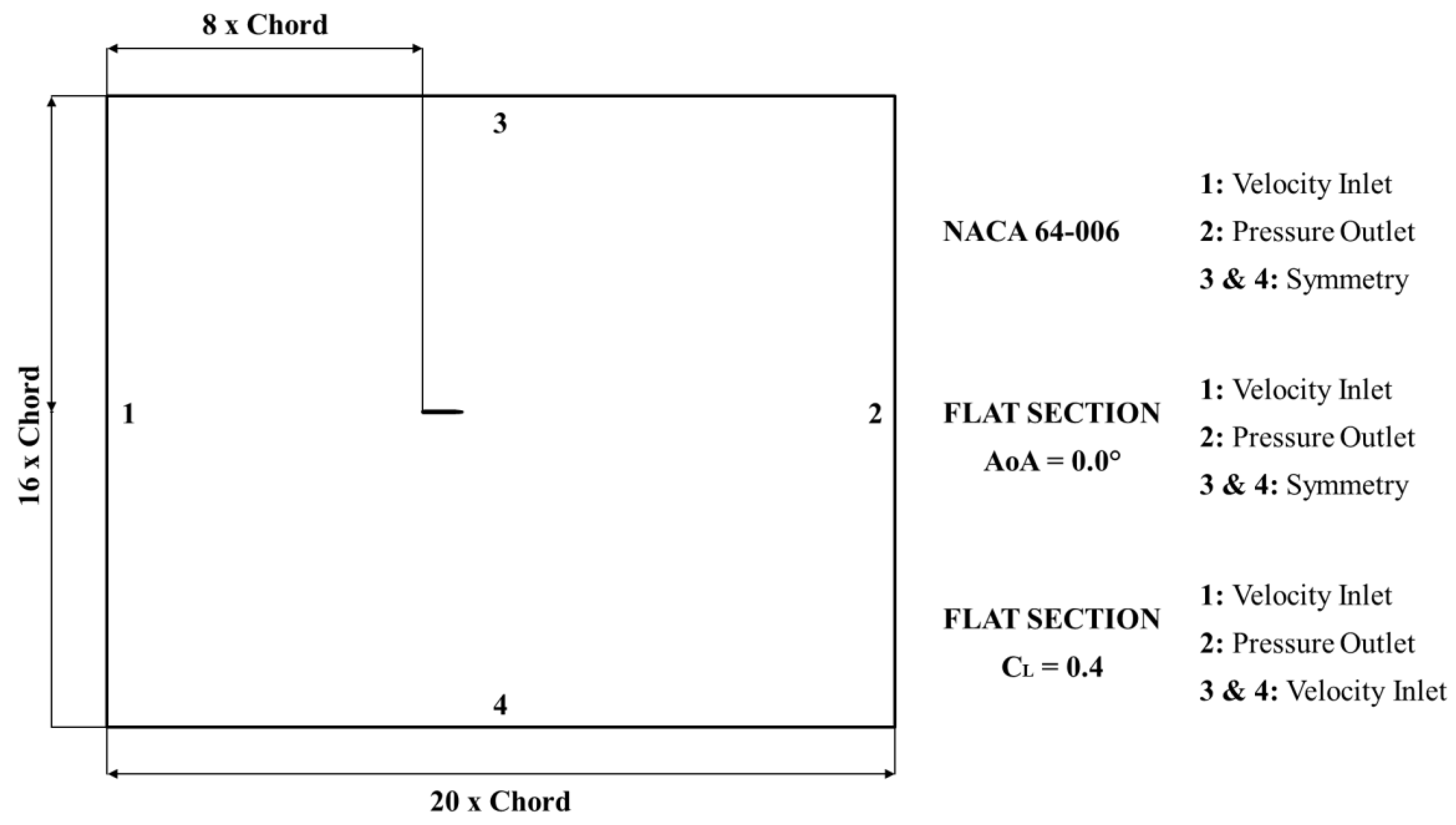
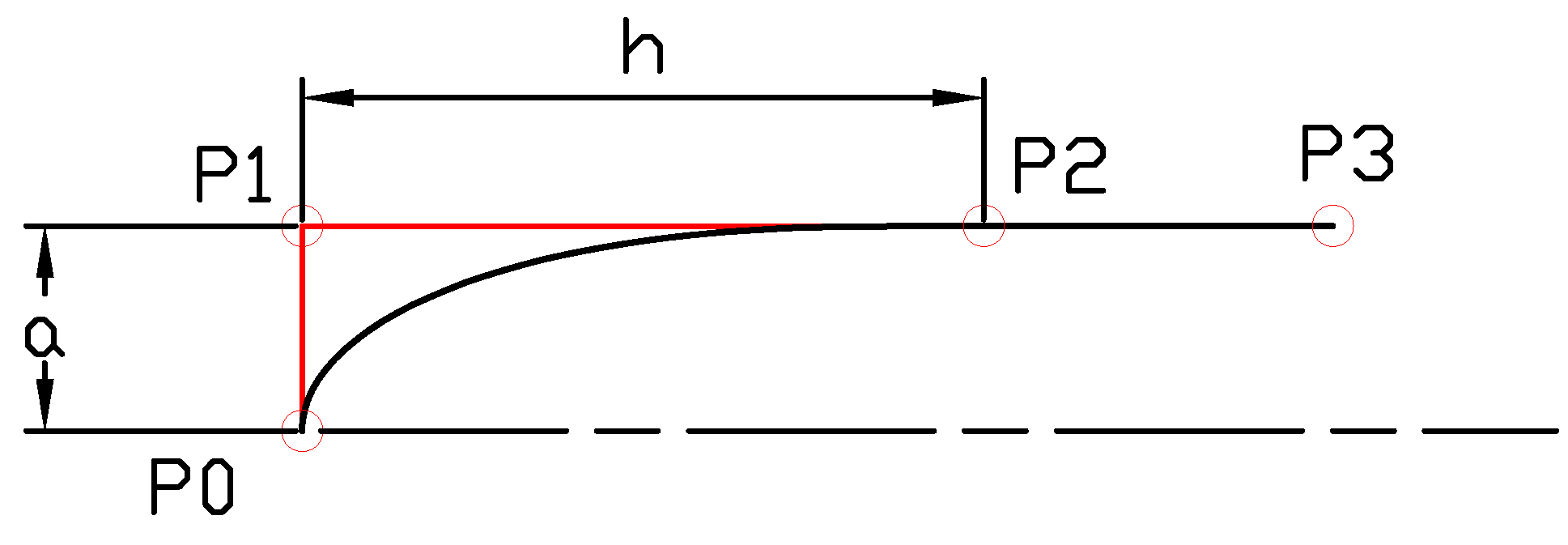
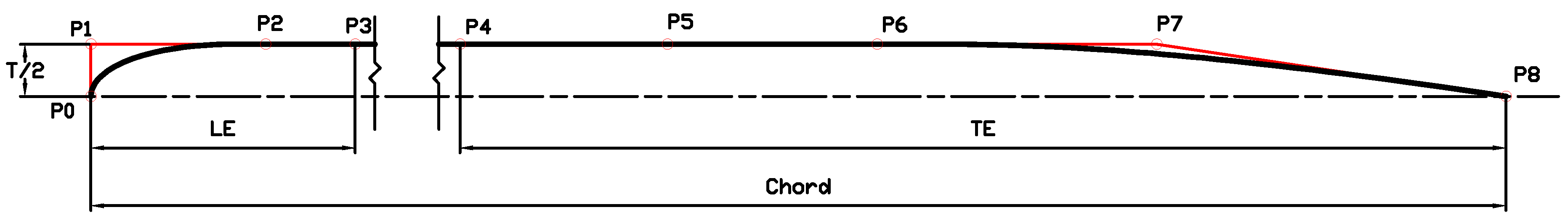
Funding

This study received funding from the Chalmers University of Technology Foundation for the Strategic Research project Hydro- and Aerodynamics. It was also partly funded by Hugo Hammar’s fund for international research in shipping, project number HHS280. The computations were performed on resources at Chalmers Centre for Computational Science and Engineering (C3SE) provided by the Swedish National Infrastructure for Computing (SNIC).

Acknowledgments

The first author gratefully acknowledges the invitation by Chalmers University of Technology and SSPA and the help and contributions by the staff duringhis six months’ visiting period as a PhD student of the University of Palermo.

Conflicts of Interest

The authors declare no conflict of interest.

Nomenclature

SymbolDefinition
CDDrag Coefficient
CLLift Coefficient
αAngle of Attack
HiRefinement Ratio
UNumerical Uncertainty
C(t)Parametric Curve
B(t)Bernstein polynomials
k(t)Curvature
wWeight of a Control Point
TThickness
LELeading Edge Length
TETrailing Edge Length
RNose Radius
ATrailing Edge Angle
AREFTrailing Edge Angle (Reference)

Appendix A. Parametric Section Design

A rational Bézier curve can be defined [21] as shown in Equation (A1):
C ( t ) = i = 0 n w i B i , n ( t ) P i i = 0 n w i B i , n ( t ) , t = 0 , , 1
where n is the degree of the curve, Pi are the coordinates of n + 1 control points, wi are the weights of the control points and B(i,n) (t) are the Bernstein polynomials over the parametric abscissa, t, whose definition is given in Equation (A2):
B i , n ( t ) = n ! i ! ( n i ) ! t i ( 1 t ) n i , i = 0 , 1 , , n
In the case of third- and fourth-degree curves, Equation (A2) gives:
B i , 3 ( t ) B i , 4 ( t )
B 0 , 3 ( t ) = ( 1 t ) 3 B 0 , 4 ( t ) = ( 1 t ) 4
B 1 , 3 ( t ) = 3   t   ( 1 t ) 2 B 1 , 4 ( t ) = 4   t   ( 1 t ) 3
B 2 , 3 ( t ) = 3   t 2   ( 1 t ) B 2 , 4 ( t ) = 6   t 2   ( 1 t ) 2
B 3 , 3 ( t ) = t 3 B 3 , 4 ( t ) = 4   t 3   ( 1 t )
B 4 , 4 ( t ) = t 4
A cubic curve (n = 3) is selected to define the shape of the leading edge of the profile. There are two reasons leading to this choice: the needs to assure G2 continuity of the profile between the leading edge and the flat zone, and the control of the curvature at the beginning of the profile. The G2 continuity is obtained by assuring that the two neighboring curves have the same tangent line and also the same center of curvature at their common boundary. The control of the curvature at the beginning of the profile is obtained with the following Equation (A3):
k ( t 0 ) = w 0 w 2 w 1 2 n 1 n h a 2
where k ( t 0 ) is the curvature, while h and a are defined in Figure A1.
Figure A1. Leading edge designed with a rational cubic Bézier curve.
Jmse 08 00677 g0a1
In this specific case, k ( t 0 ) = 1 R , a = y P 1 and h = y P 2 . Equation (A3) can be solved to obtain the correct value of the weight w1 of the control point P1, according to Equation (A4).
w 1 = 2   R   x P 2   w P 0   w P 2 3   y P 2 2
Table A1 shows the values of the coordinates of each control point of the leading edge and the corresponding weights.
Table A1. Coordinates and weights of leading edge control points.
Leading Edge
Control PointxyWeight
P0001
P10 T 2 2   R   x P 2   w P 0   w P 2 3   y P 2 2
P2 2   LE 3 T 2 1
P3 LE T 2 1
A fourth-degree (n = 4) curve is selected to define the shape of the trailing edge of the profile. In the same way as the leading edge, the G2 continuity is assured. A higher degree is needed to control the trailing edge angle at the end of the profile without violating the G2 continuity. The shape of the trailing edge can be seen in Figure A2, while Equation (A5) shows how to properly obtain the value of the trailing edge angle.
Figure A2. Trailing edge designed with a rational Bézier curve.
Jmse 08 00677 g0a2
A = arctan ( y P 7 x P 8 x P 7 )
Table A2 shows the values of the coordinates of each control point of the trailing edge and the corresponding weights.
Table A2. Coordinates and weights of trailing edge control points.
Trailing Edge
Control PointxyWeight
P40 T 2 1
P5 x P 6 2 T 2 1
P6 T E 2.5 T 2 1
P7 2   T E 3 ( x P 8 x P 7 )   tan ( A ) 1
P8 T E 01
In Figure A3, the whole flat section is shown. It is obtained by translating the values of the coordinate points of the trailing edge by a quantity equal to the leading edge length plus the length of the flat zone of the profile.
Figure A3. Flat section designed with three rational Bézier curves.
Jmse 08 00677 g0a3
A reference value for the trailing edge angle is AREF, defined by Equation (A5) for y P 7 = T 2 , i.e., it may be computed as
A R E F = arctan ( T 2 T E 2 T E 3 ) =   arctan ( 1.5 T T E )
To define the profile of a parallel-sided section, rational Bézier curves are defined and linked to the geometrical variables of the problem: thickness (T), leading edge length (LE), trailing edge length (TE), nose radius (R) and trailing edge angle (A). T, LE, TE are expressed in percent of the chord, and R is expressed in percent of the thickness. A is expressed as a fraction of AREF. The shape of the profile is completely parameterized, so it is possible to automatically generate all 200 shapes needed for the present study. Since this technique is very versatile, it can easily be implemented in different cases from the one presented here. A code, developed in Excel VBA, starts from the values of the design variables, processes this information to define the geometry of each curve, and saves the data for each of the sections in a neutral CAD format (e.g., IGES, CSV). Figure A4 shows the geometry of one section. As can be seen, it has been divided into three main zones: leading edge, flat zone, trailing edge. The length of each zone is related to the class rules of each dinghy. The red dots represent the control points of the curve, while the blue ones represent the points of the curves whose internal spacing can be modified to better follow the shape.
Figure A4. An example of the shape of a Parallel-Sided section.
Jmse 08 00677 g0a4

Appendix B. Selection of the Best Shape

Table A3, Table A4 and Table A5 show the best shapes for each Reynolds number. These can be useful for designers that can enter the desired values of thickness (T), leading edge length (LE) and trailing edge length (TE) and see what radius (R) and trailing edge angle (A) to use for minimizing the drag coefficient. Note that T, LE, TE are given in percent of the chord length, R is expressed in percent of the thickness and A as a fraction of AREF. If there are many possibilities, the tables can be useful to compare all the possible solutions and design the best one for the specific application. The best LE, TE, R and A combination for each combination of thickness, angle of attack and Reynolds number is given in bold.
Table A3. Best shapes for Reynolds number 300,000.
Re 300,000 − AoA = 0.0°Re 300,000 − CL = 0.4
TLETERACD × 103TLETERACD × 103
4102020 1 5 A R E F 8.46410205 4 5 A R E F 12.06
4104020 1 5 A R E F 6.18410405 1 5 A R E F 11.85
420202 2 5 A R E F 8.384202010 1 5 A R E F 12.28
4204010 1 5 A R E F 6.054204010 A R E F 13.21
8102020 3 5 A R E F 16.188102010 2 5 A R E F 17.78
8104020 1 5 A R E F 13.528104010 4 5 A R E F 15.89
8202010 3 5 A R E F 20.21820202 2 5 A R E F 14.01
820402 1 5 A R E F 10.64820405 1 5 A R E F 12.29
Table A4. Best shapes for Reynolds number 900,000.
Re 900,000 − AoA = 0.0°Re 900,000 − CL = 0.4
TLETERACD × 103TLETERACD × 103
410205 2 5 A R E F 5.474102010 1 5 A R E F 9.30
410405 2 5 A R E F 3.714104010 1 5 A R E F 8.36
420202 2 5 A R E F 5.434202010 4 5 A R E F 10.05
420402 2 5 A R E F 3.69420405 3 5 A R E F 9.13
8102040 2 5 A R E F 12.148102010 3 5 A R E F 13.79
8104040 1 5 A R E F 10.748104040 1 5 A R E F 10.22
8202020 3 5 A R E F 14.288202010 3 5 A R E F 12.55
820402 2 5 A R E F 5.01820405 2 5 A R E F 8.48
Table A5. Best shapes for Reynolds number 1,500,000.
Re 1,500,000 − AoA = 0.0°Re 1,500,000 − CL = 0.4
TLETERACD × 103TLETERACD × 103
410205 2 5 A R E F 3.80410205 1 5 A R E F 8.71
410402 3 5 A R E F 2.94410405 1 5 A R E F 8.06
4202010 2 5 A R E F 3.784202010 1 5 A R E F 8.83
420402 3 5 A R E F 2.934204010 1 5 A R E F 8.17
8102040 2 5 A R E F 10.818102020 2 5 A R E F 10.47
8104040 1 5 A R E F 9.688104020 2 5 A R E F 8.50
8202020 2 5 A R E F 10.158202010 1 5 A R E F 10.12
820402 3 5 A R E F 3.798204010 2 5 A R E F 7.48
With the information presented in the tables, it is possible to find a good set of parameters for a given dinghy. For example, as seen in Table 3, the Optimist centerboard has a Reynolds number near 300,000, so Table A3 should be used. The maximum trailing edge length is 21.43% of the chord, so TE2 cannot be used. Considering the upwind condition (CL = 0.4), the best computed configuration is: T = 4, LE = 10, TE = 20, R = 5, A = 4 5 A R E F . For the downwind condition (AoA = 0.0), the best computed configuration is: T = 4, LE = 20, TE = 20, R = 2, A = 2 5 A R E F . It is important to consider the fact that, during the downwind leg of a regatta, it is common practice to partially hoist the centreboard in order to reduce the wetted surface, so the designer should give more importance to the upwind configuration.

References

  1. Abbott, I.H.; von Doenhoff, A.E. Theory of Wing Sections; Dover Publications INC.: New York, NY, USA, 1959. [Google Scholar]
  2. World Sailing Class Association. International 470 Class Rules; World Sailing Class Association: Paris, France, 2017. [Google Scholar]
  3. World Sailing Class Association. International 420 Class Rules; World Sailing Class Association: Paris, France, 2017. [Google Scholar]
  4. International Optimist Dinghy Association. International Optimist Class Rules; International Optimist Dinghy Association: Paris, France, 2018. [Google Scholar]
  5. Pollok, N.A. Note on the Aerodynamic Design of Thin Parallel-Sided Aerofoil Sections; Aerodynamics NACA Technical Memorandum 388; Aeronautical Research Labs: Melbourne, Australia, 1987. [Google Scholar]
  6. Drela, M. XFOIL Subsonic Airfoil System. Available online: https://web.mit.edu/drela/Public/web/xfoil/ (accessed on 31 May 2019).
  7. Larsson, L.; Eliasson, R.E.; Orych, M. Principles of Yacht Design; Adlard Coles Nautical Ltd.: London, UK, 2014. [Google Scholar]
  8. Larsson, L.; Raven, H. Ship Resistance and Flow; Principles of Naval Architecture Series; SNAME: Hoboken, NJ, USA, 2010. [Google Scholar]
  9. Siemens. Simcenter STAR-CCM+ Documentation, Version 2020.1, 2020.
  10. Menter, F.R. Two-equation eddy-viscosity turbulence models for engineering applications. AIAA J. 1994, 32, 1598–1605. [Google Scholar] [CrossRef] [Green Version]
  11. Larsson, L.; Stern, F.; Visonneau, M. Numerical Ship Hydrodynamics—An Assessment of the Gothenburg 2010 Workshop; Springer: Doordrecht, Germany, 2014. [Google Scholar]
  12. Hino, T.; Stern, F.; Larsson, L.; Visonneau, M.; Hirata, N.; Kim, J. Numerical Hydrodynamics—An Assessment of the Tokyo 2015 Workshop; Springer: Cham, Switzerland, 2020. [Google Scholar]
  13. Marvin, J.G. Book review turbulence modeling for CFD. AIAA J. 1994, 32, 1339. [Google Scholar] [CrossRef]
  14. Menter, F.R.; Langtry, R.B.; Likki, S.R.; Suzen, Y.B.; Huang, P.G.; Völker, S.A. Correlation-based transition model using local variables—Part I: Model formulation. J. Turbomach. 2006, 128, 413–422. [Google Scholar] [CrossRef]
  15. Menter, F.R.; Smirnov, P.E.; Liu, T.; Avancha, R. A one-equation local correlation-based transition model. Flow Turbul. Combust. 2015, 95, 583–619. [Google Scholar] [CrossRef]
  16. Von Doenhoff, A.E.; Albert, E.; Abbott, F.T., Jr. The Langley Two-Dimensional Low-Turbulence Pressure Tunnel; NACA TN No. 1283; NASA Langley Research Center: Hampton, VA, USA, 1947. [Google Scholar]
  17. Remmlinger, U. The Factors that Trigger the Transition to Turbulent Flow on the Keel of a Sailing Yacht, 2013; unpublished.
  18. ITTC. Uncertainty Analysis in CFD Verification and Validation Methodology and Procedures, International Towing Tank Conference. 2017.
  19. Xing, T.; Stern, F. Closure to Discussion of ‘Factors of Safety for Richardson Extrapolation’. ASME J. Fluids Eng. 2011, 133, 115502. [Google Scholar] [CrossRef]
  20. Eça, L.; Hoekstra, M. A procedure for the estimation of the numerical uncertainty of CFD calculations based on grid refinement studies. J. Comput. Phys. 2014, 262, 104–130. [Google Scholar] [CrossRef]
  21. Sederberg, T.W. Computer Aided Geometric Design; Computer Aided Geometric Design Course Notes; BYU Scholars Archive, 2012. [Google Scholar]
Figure 1. Boundary definition.
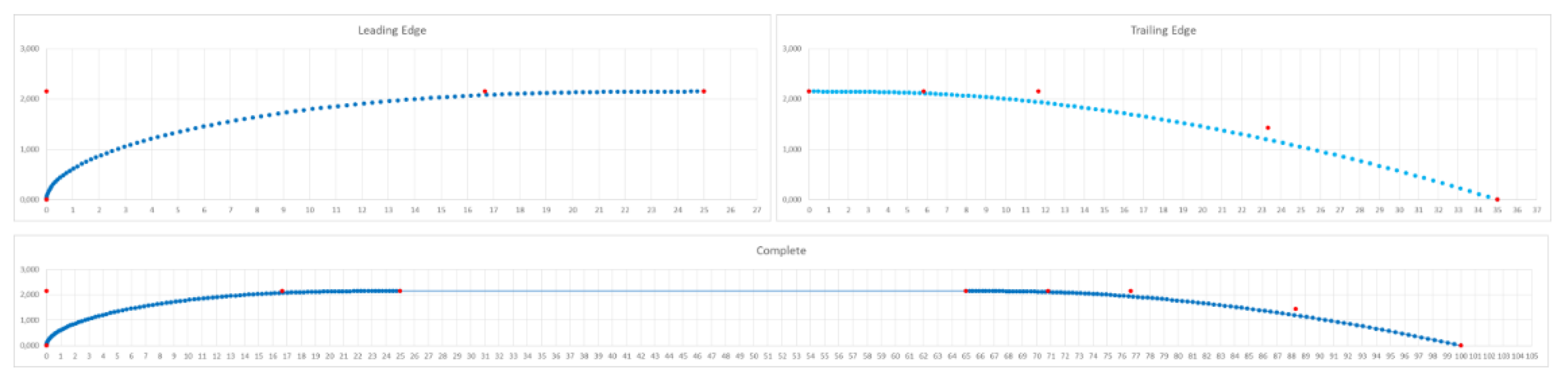
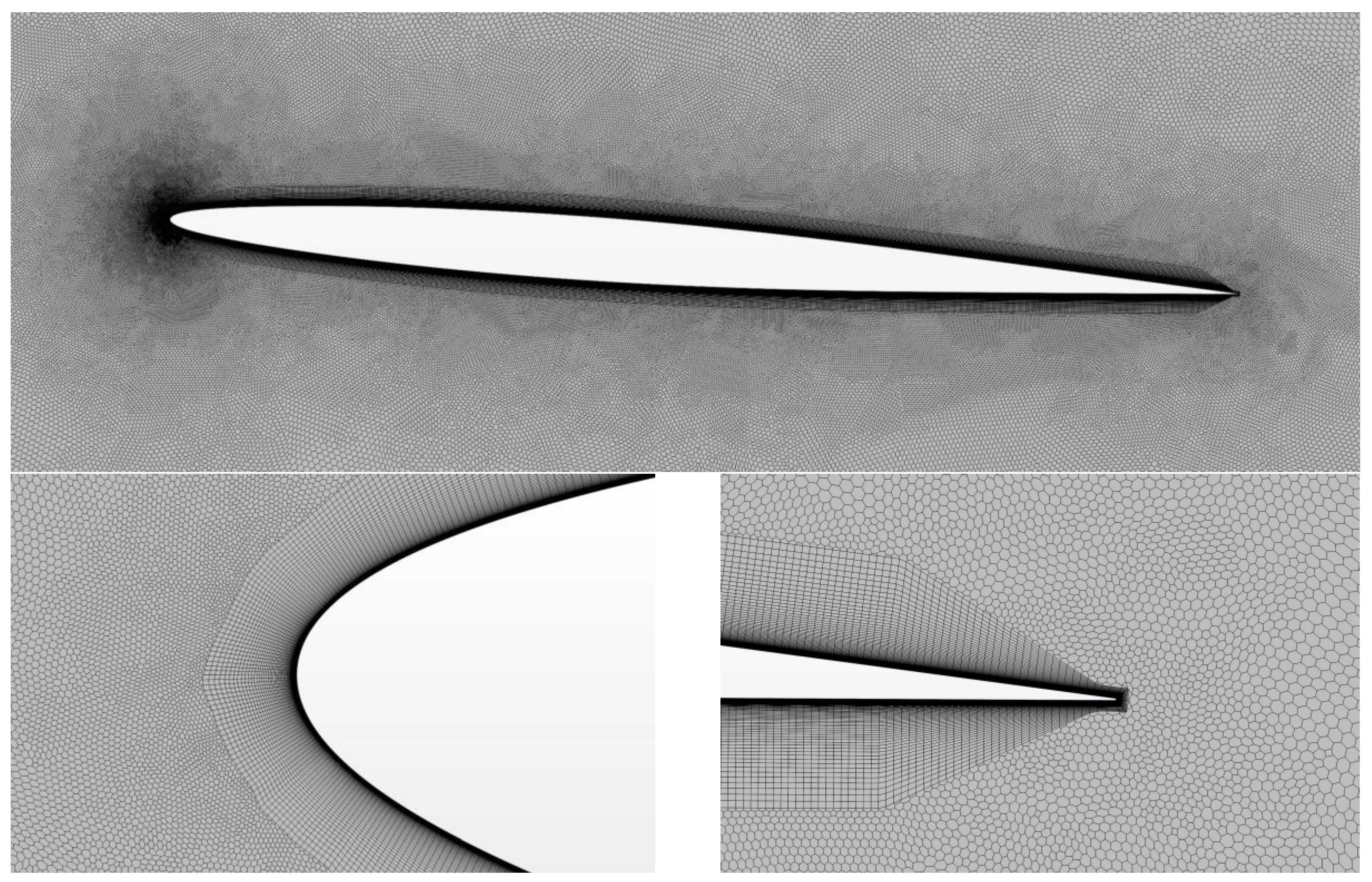
Jmse 08 00677 g001
Figure 2. View of the mesh surrounding the test case section, and close-ups of leading and trailing edges. For the test case, the angle of attack is achieved by rotation of the foil, while for the systematic computations the direction of the inflow is varied to obtain the requested lift coefficient (0.4).
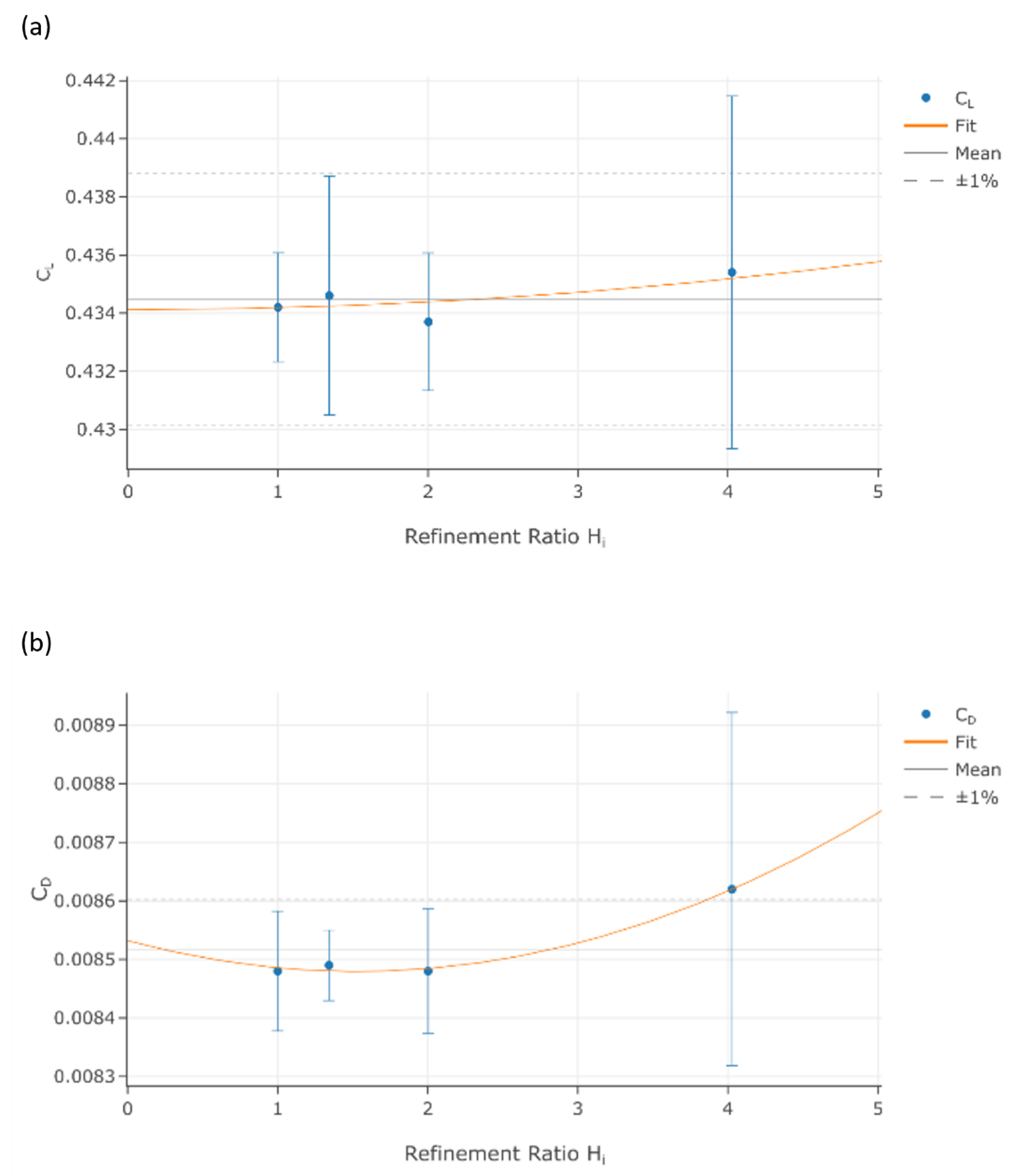
Jmse 08 00677 g002
Figure 3. Regression curve of lift coefficient (a) and drag coefficient (b).
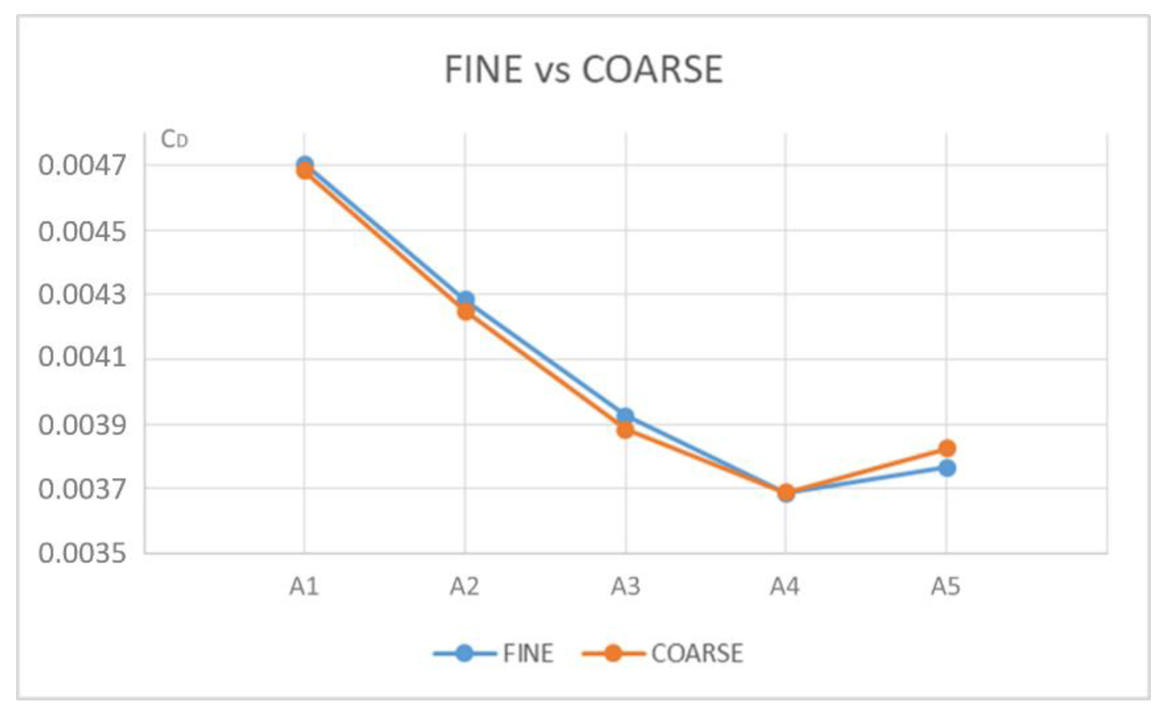
Jmse 08 00677 g003
Figure 4. Comparison of drag coefficients for the coarse grid and a finer one. The independent variable is the trailing edge angle (see below).
Jmse 08 00677 g004
Figure 5. Comparison between numerical and experimental results. Reynolds number 3,000,000.
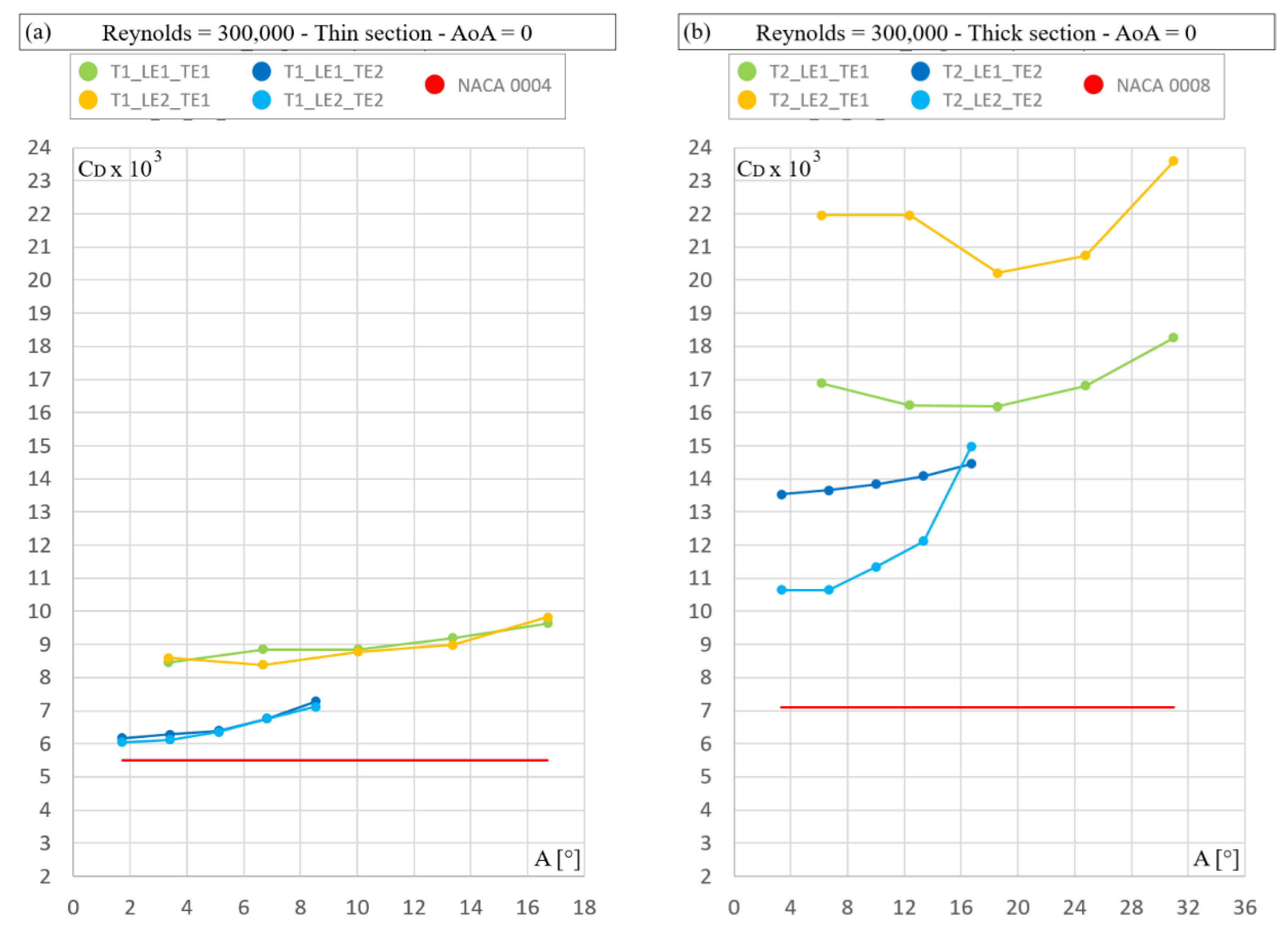
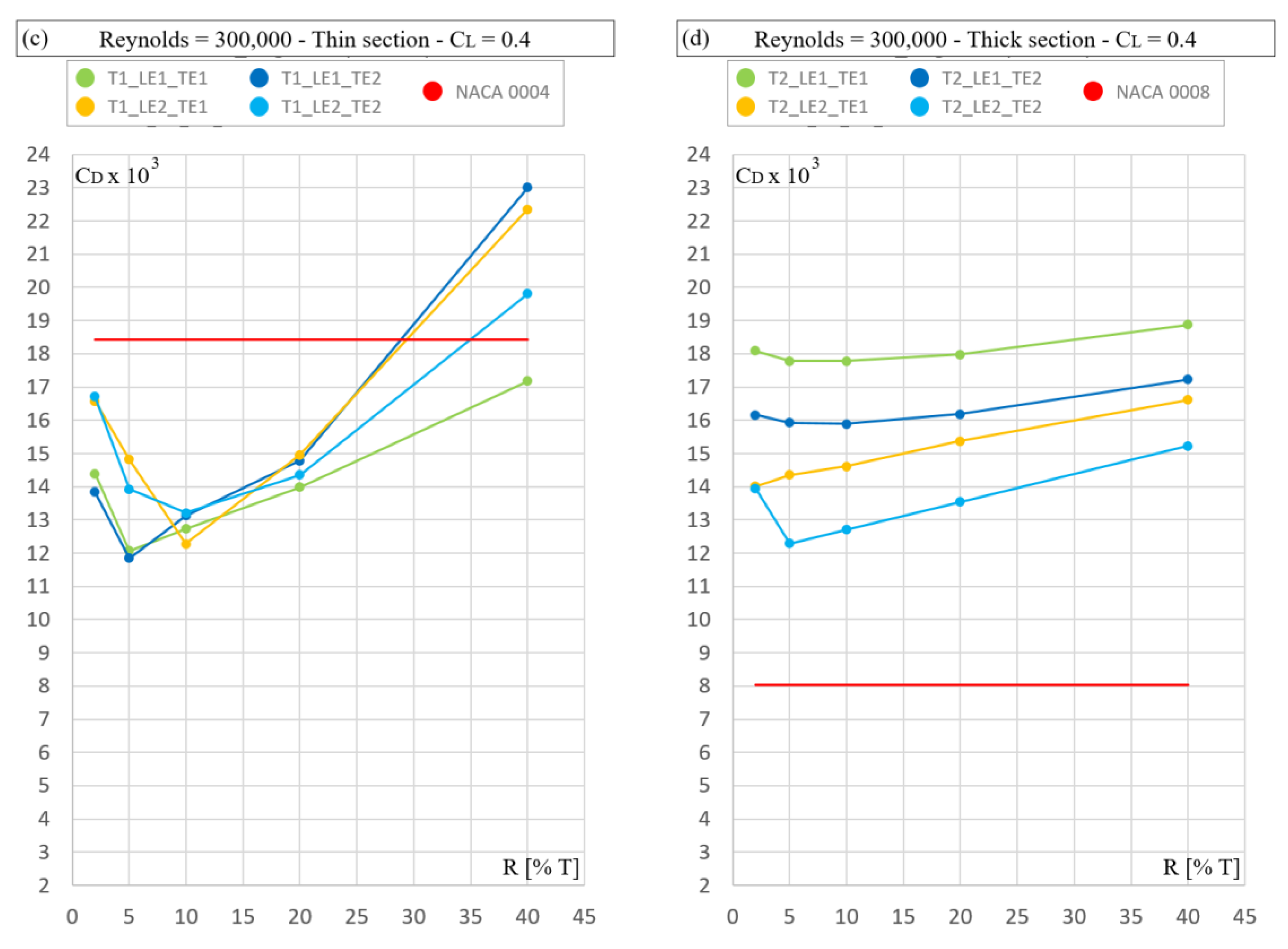
Jmse 08 00677 g005
Figure 6. Drag coefficient (CD × 103) for Reynolds number 300,000. Independent variable: trailing edge angle (a,b); nose radius (c,d).
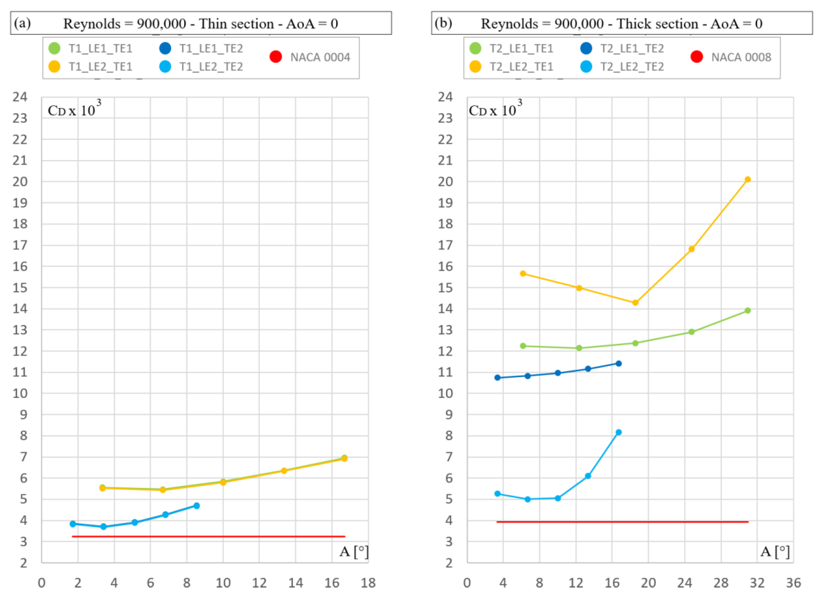
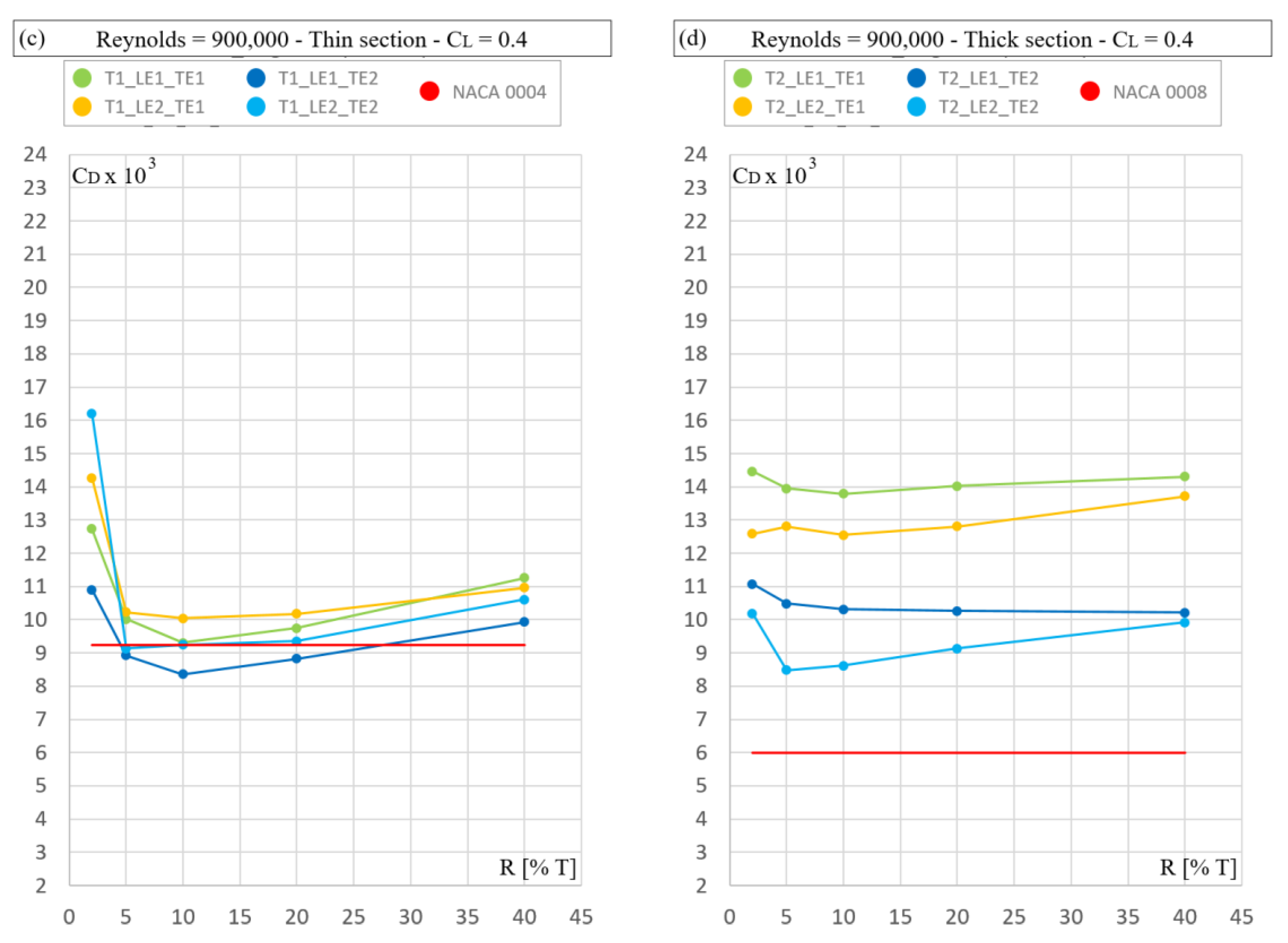
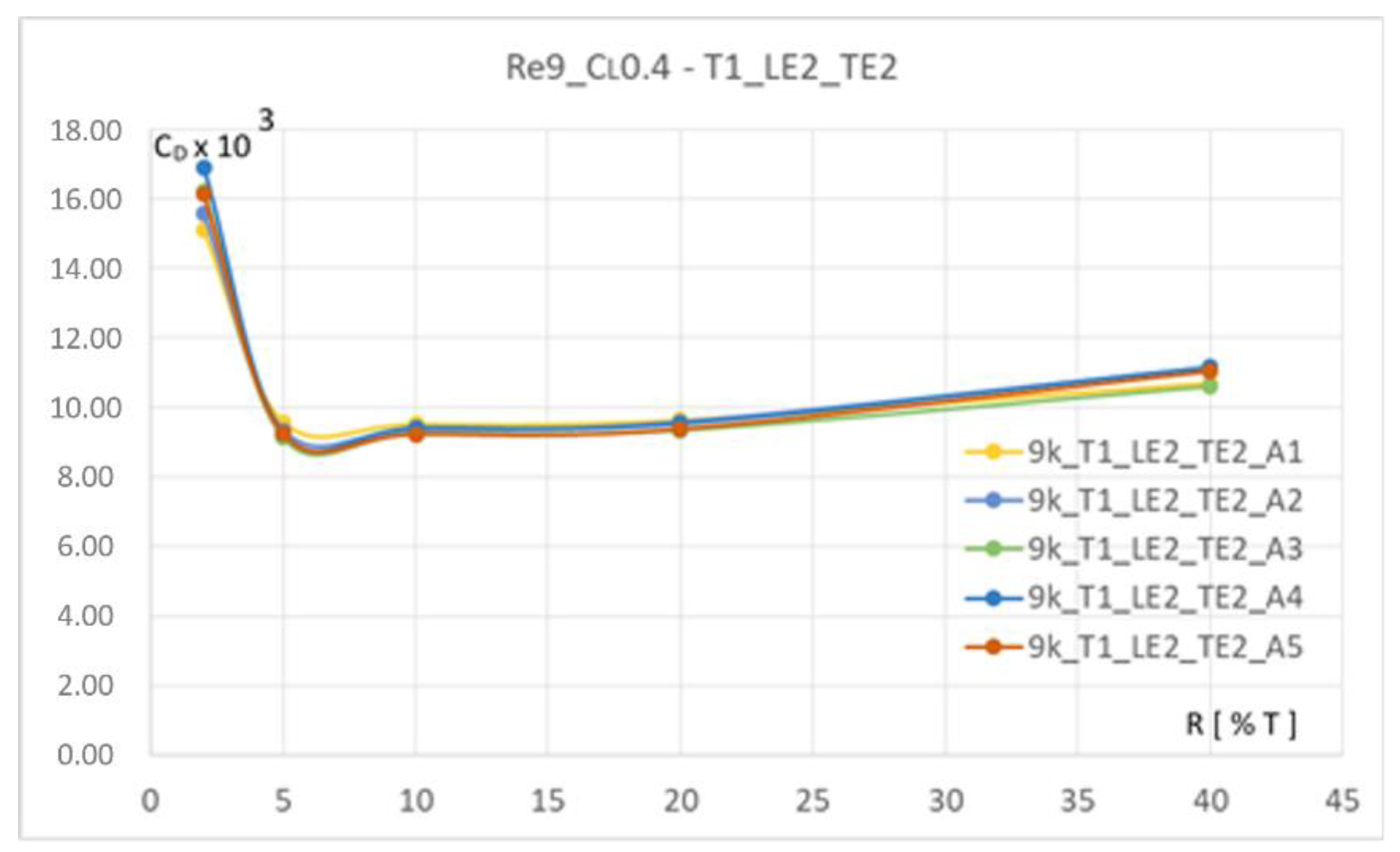
Jmse 08 00677 g006aJmse 08 00677 g006b
Figure 7. Drag coefficient (CD × 103) for Reynolds number 900,000. Independent variable: trailing edge angle (a,b); nose radius (c,d).
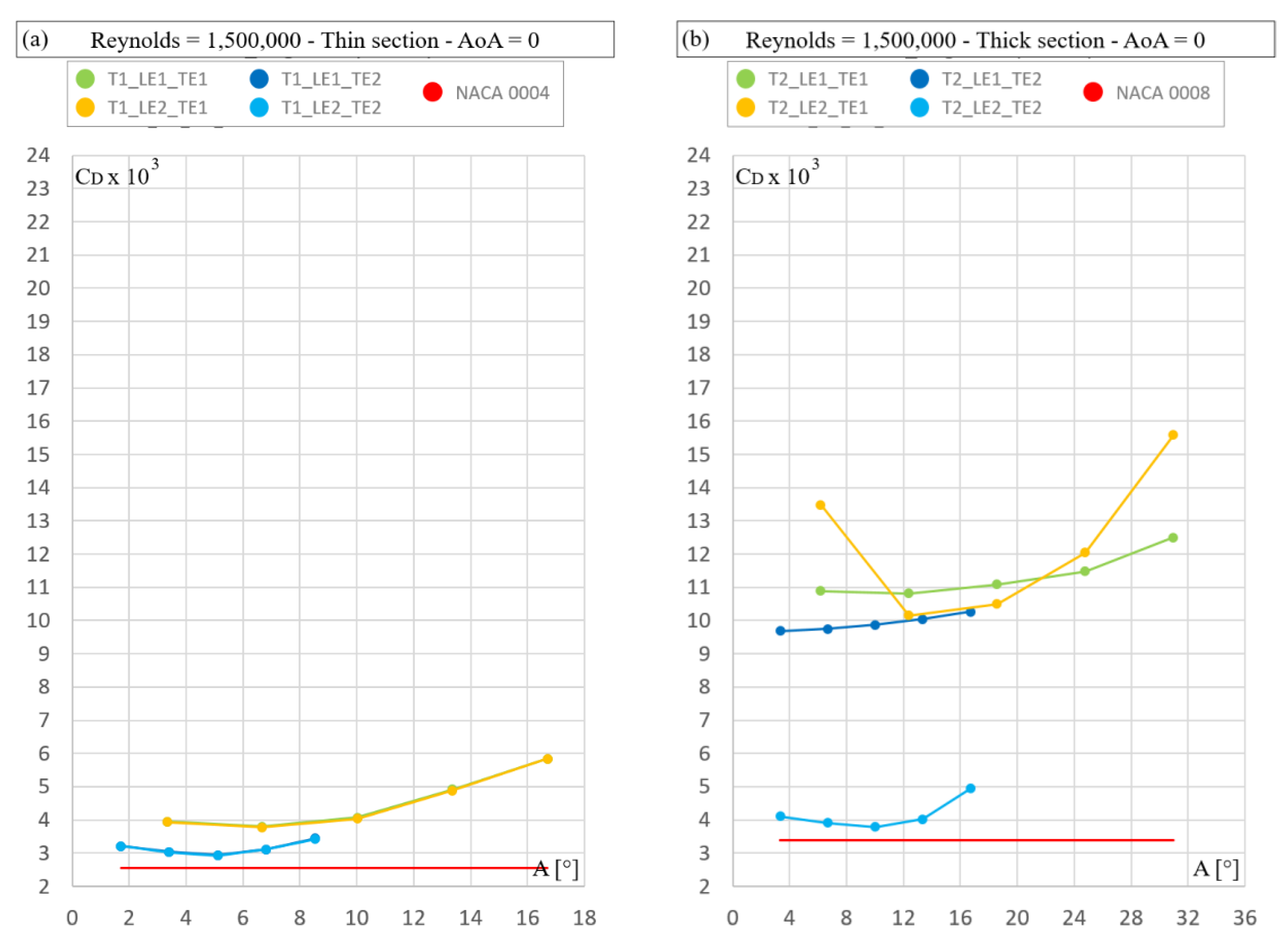
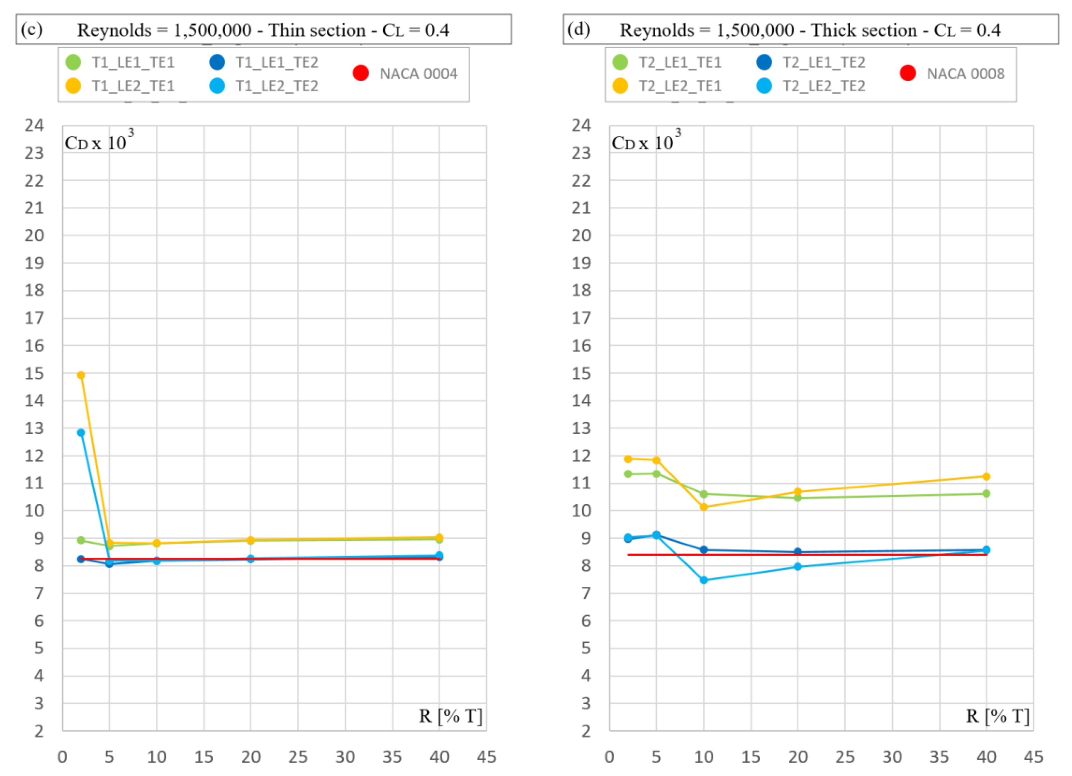
Jmse 08 00677 g007aJmse 08 00677 g007b
Figure 8. Drag coefficient (CD × 103) for Reynolds number 1,500,000. Independent variable: trailing edge angle (a,b); nose radius (c,d).
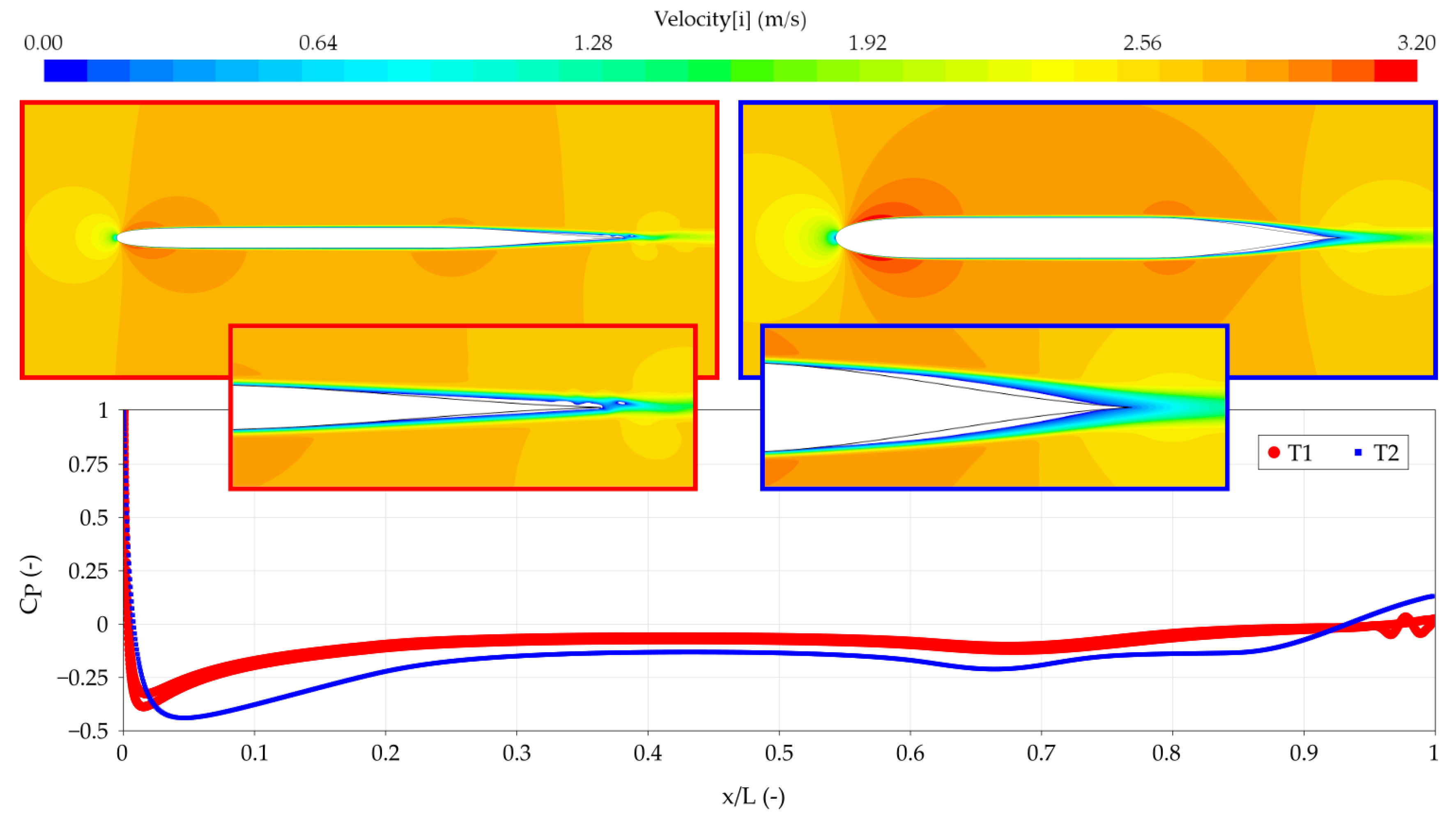
Jmse 08 00677 g008aJmse 08 00677 g008b
Figure 9. Plots of axial velocity (upper) and pressure distribution (lower) for a thin and a thick section.
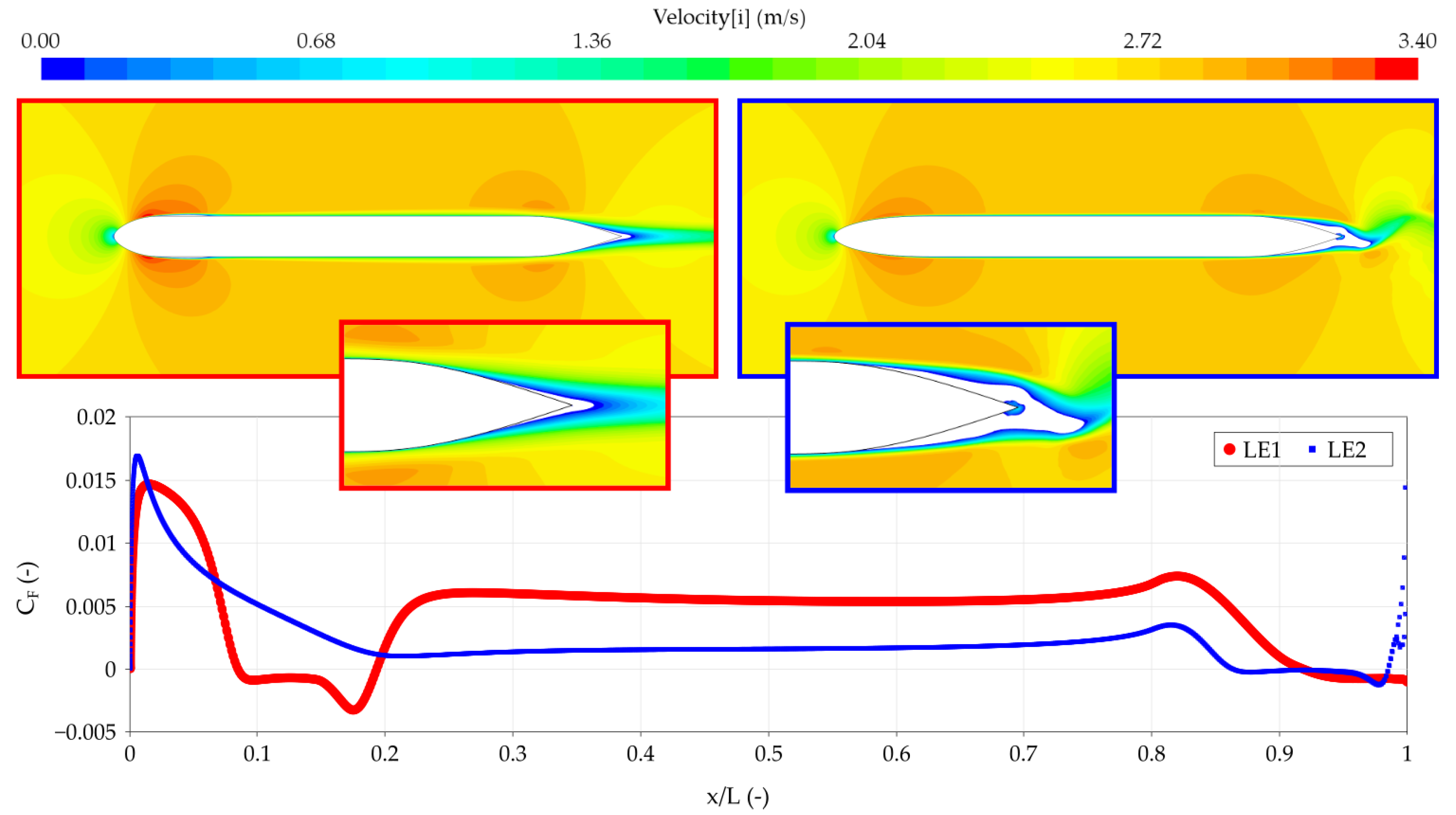
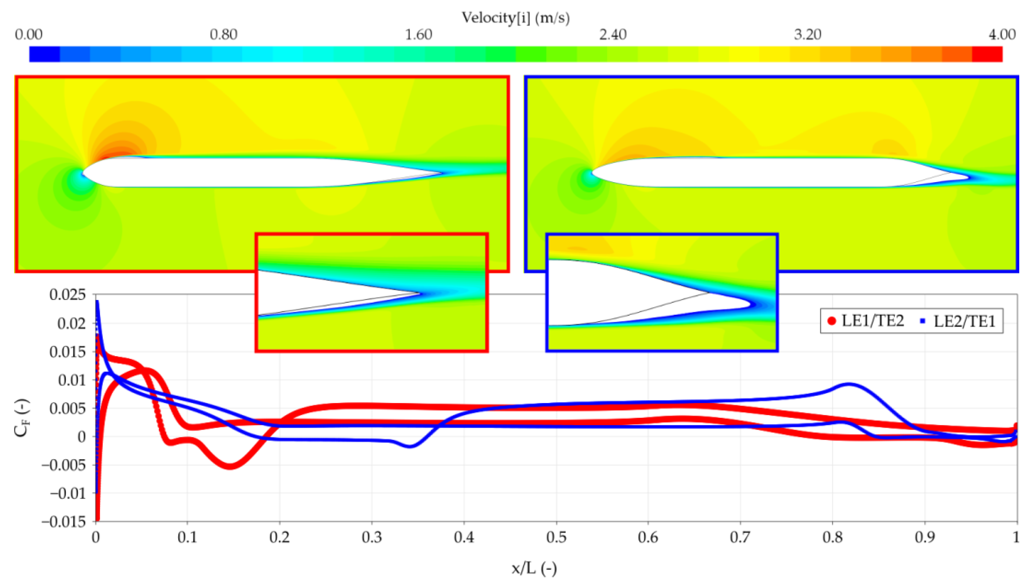
Jmse 08 00677 g009
Figure 10. Velocity plot and skin friction coefficient of short leading edge length (left) and long leading edge length (right).
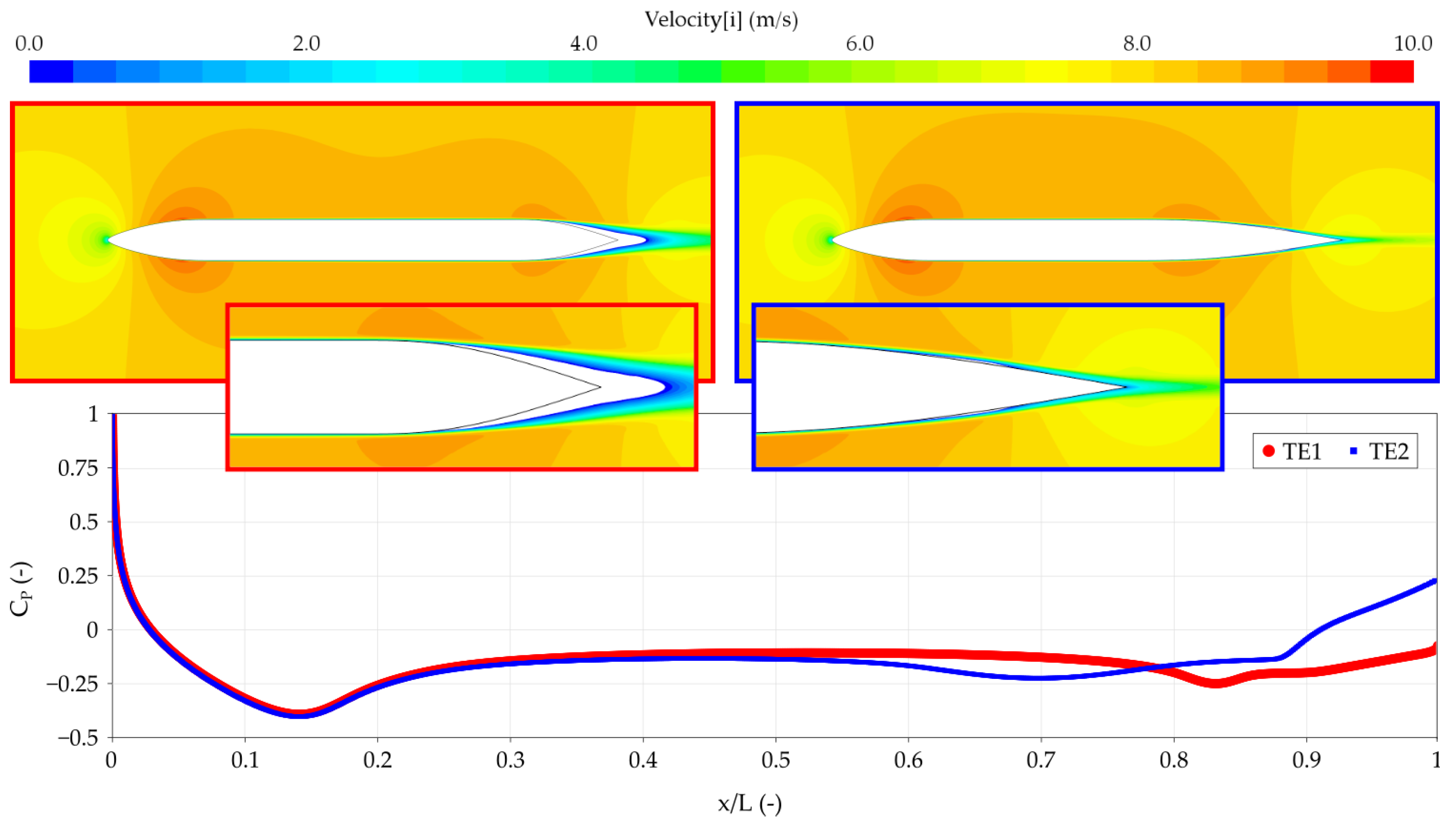
Jmse 08 00677 g010
Figure 11. Velocity plot and pressure plot of short trailing edge (left) and long trailing edge (right) sections.
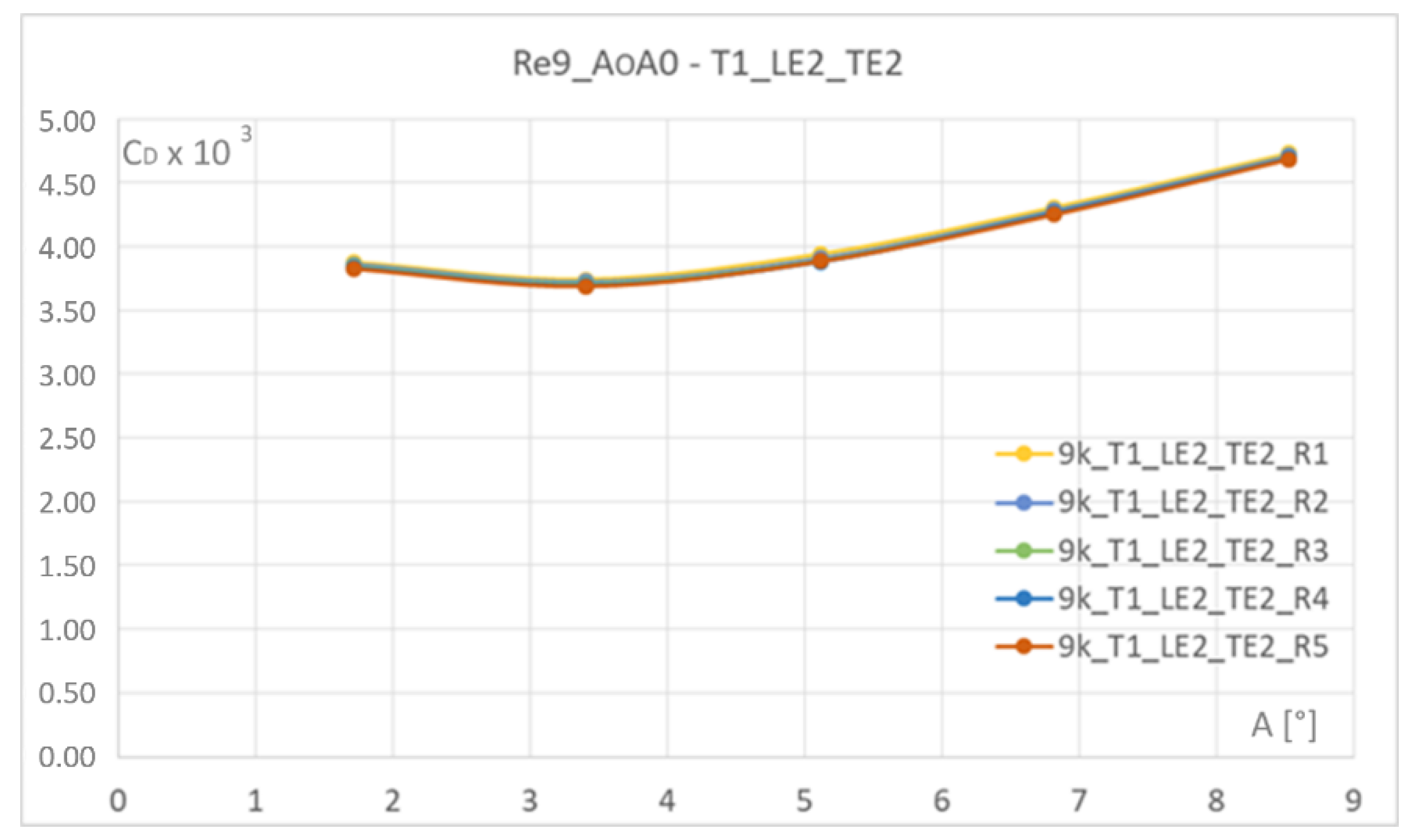
Jmse 08 00677 g011
Figure 12. Five different radii are compared. x-axis trailing edge angle, y-axis drag coefficient times 103.
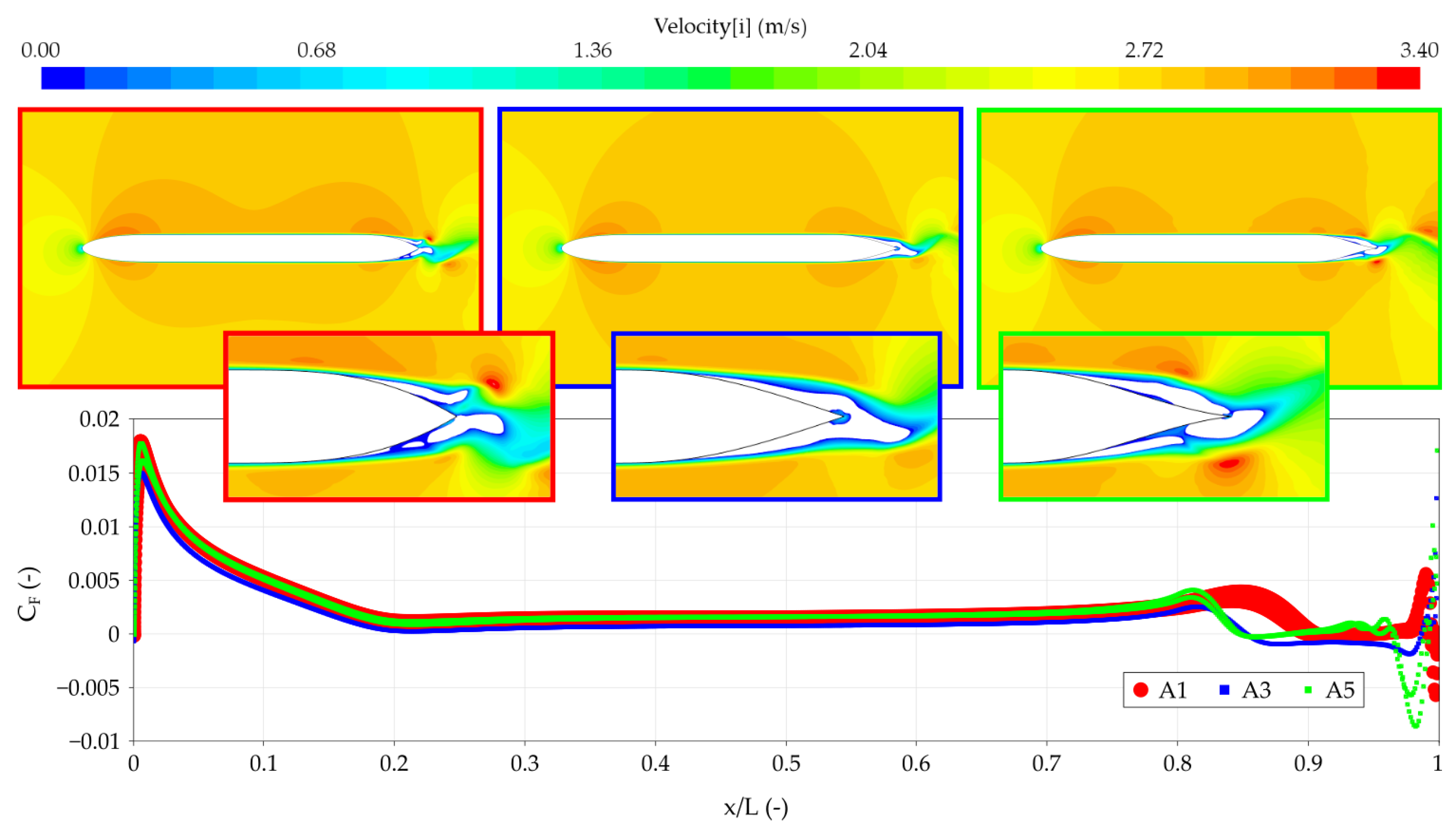
Jmse 08 00677 g012
Figure 13. Velocity plot and skin friction coefficient of large (left), medium (center) and small (right) trailing edge angle sections.
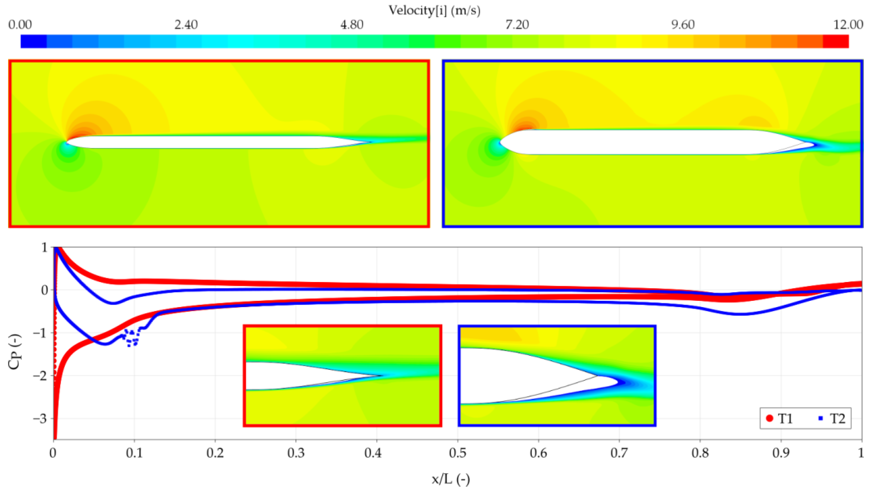
Jmse 08 00677 g013
Figure 14. Velocity plot and pressure plot of thin (left) and thick (right) sections.
Jmse 08 00677 g014
Figure 15. Velocity plot and skin friction coefficient of short leading edge and long trailing edge (left) and long leading edge and short trailing edge (right) sections.
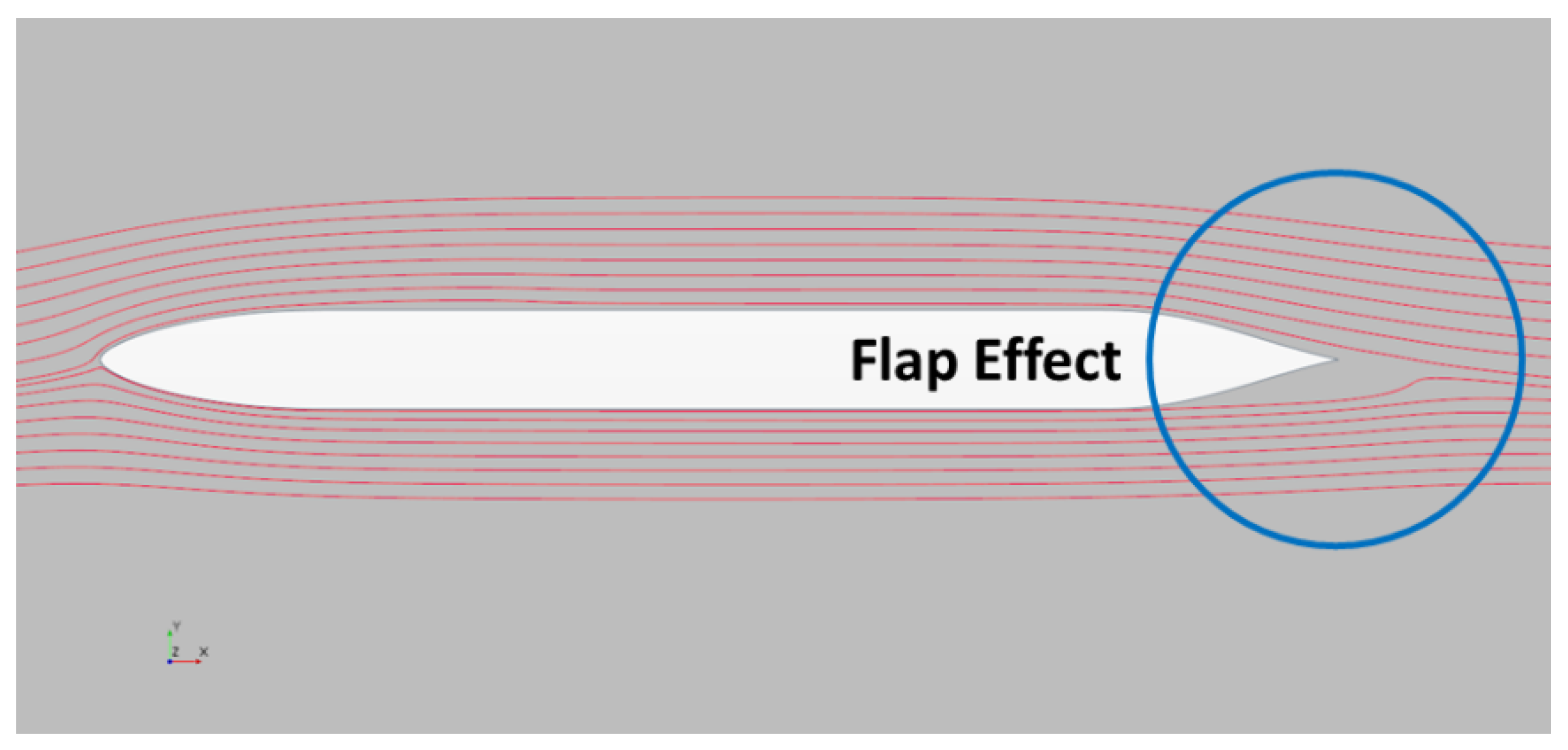
Jmse 08 00677 g015
Figure 16. Streamlines of long leading edge and short trailing edge section.
Jmse 08 00677 g016
Figure 17. Five different trailing edge angles are compared, x-axis nose radius, y-axis drag coefficient times 103.
Jmse 08 00677 g017
Figure 18. Velocity plot and pressure plot of short leading edge (left) and long leading edge (right) sections.
Jmse 08 00677 g018
Table 1. Numerical uncertainty of lift and drag coefficient for the test case at different grid densities.
Nr. CellsHiCLU (CL)U (%CL)CDUU (%CD)
6.5 M10.43540.001870.50.008500.0001021.2
3.6 M1.340.43370.004110.90.008490.0000600.7
1.6 M20.43460.002370.50.008480.0001061.3
0.4 M4.030.43420.006061.40.008620.0003013.5
Table 2. Numerical and experimental results for different angle of attack.
Angle of AttackTest CaseAbbott
αCDCD
0.00.003440.0039
1.00.003480.0040
1.50.003520.0050
2.00.003620.0060
2.50.006400.0062
3.00.006700.0063
4.00.007700.0069
Table 3. Ranges of Reynolds numbers, thicknesses, leading edge lengths, trailing edges lengths of 470, 420 and Optimist dinghies.
BoatReynolds NumberThickness (% Chord)Leading Edge (% Chord)Trailing Edge (% Chord)
Optimist280,0005.5221.4321.43
290,0007.1420.6920.69
420830,0003.7625.3025.30
850,0004.8224.7124.71
470910,0004.2618.0835.49
1,500,0007.8911.7022.97
Table 4. Values and codes for the systematic investigation of Parallel-Sided sections.
Reynolds NumberSailing ConditionThickness (% Chord)Leading Edge (% Chord)Trailing Edge (% Chord)Nose Radius (% Thickn.)Trailing Edge Angle [°]
300,000AoA = 0.0°T1 = 4%LE1 = 10%TE1 = 20%R1 = 40%A1 = AREF
900,000CL = 0.4T2 = 8%LE2 = 20%TE2 = 40%R2 = 20%A2 = 4 5 AREF
1,500,000----R3 = 10%A3 = 3 5 AREF
-----R4 = 5%A4 = 2 5 AREF
-----R5 = 2%A5 = 1 5 AREF

