A Geometric Calibration Method of Hydrophone Array Based on Maximum Likelihood Estimation with Sources in Near Field

Abstract

Considering the requirement of the near-field calibration under strong underwater multipath condition, a high-precision geometric calibration method based on maximum likelihood estimation is proposed. It can be used as both auxiliary-calibration and self-calibration. According to the near-field geometry error model, the objective function of nonlinear optimization problem is constructed by using the unconditional maximum likelihood estimator. The influence of multipath on geometric calibration is studied. The strong reflections are considered as the coherent sources, and the compensation strategy for auxiliary-calibration is realized. The optimization method (differential evolution, DE) is used to solve the geometry errors and sources’ position. The method in this paper is compared with the eigenvector method. The simulation results show that the method in this paper is more accurate than the eigenvector method especially under high signal-to-noise ratio (SNR) and multipath environment. Experiment results further verify the effectiveness.

1. Introduction

For the hydrophone array, the array error mainly includes the array amplitude errors, phase errors, and the geometry errors, which is one of the important factors affecting the array processing capability [1]. Array calibration can reduce this kind of error and ensure high-precision measurement. At present, most array calibration methods consider far-field plane wave condition [2]. However, for sonar systems with large aperture, far-field conditions are not easily met, especially in water pool or other space-constrained conditions. Model mismatch will occur when the distance is insufficient between the source and the array [3]. In addition, the near-field calibration has a higher signal-to-noise ratio (SNR) than the far-field calibration, which can improve the calibration accuracy. Therefore, it is significant to develop an array calibration method utilizing near-field sources.

The earliest array calibration method is realized by measuring, interpolating, and storing the actual array manifold, but this method needs to be measured in the use environment [4]. If there is mismatch between the measurement and the application environment, the calibration effect will be seriously affected. Its operation is difficult and the accuracy is not ideal. In the 1990s, scholars tried to parameterize the array manifold error by means of mathematical modeling, transforming the array calibration problem into a parameter estimation problem [5]. They analyzed the correctable conditions of different arrays [6] and Cramer-Rao Lower Bound (CRLB) [7] of different calibration models.

According to the type of calibration source, array calibration can be divided into auxiliary calibration and self-calibration.

The active correction is to estimate the array errors by using the auxiliary source with known position. Its advantages are that it needs less calculation and needs less calibration source than self-calibration [8,9]. However, because it depends on the auxiliary source, its performance will decline sharply when the position of the auxiliary source is deviated. Typical auxiliary calibration methods include eigenvector calibration method [10] and subspace calibration method [11]. The former utilizes the corresponding relationship between guide vector and main eigenvector of covariance matrix, and establishes equations of the steering vector function using the array error as the variable, then solves the array error parameters. In the latter, an approximation is used to expand the steering vector into a linear or generalized linear combination of array errors, and the array error is solved according to the subspace principle, such as the noise subspace is orthogonal to the target guidance vector. Reference [12] is based on the first idea above for array correction, and uses the near-field auxiliary source. It is aimed at the perturbation error. Using the Taylor approximation, the guidance vector is expressed as a linear function of the array element position error in the near-field model. The analytical solution of the array error can be obtained. This method is simple in calculation, but only suitable for the case of small error. In [13], aiming at the problem that the performance of compact phased-array high-frequency ground-wave radars is seriously degraded by array error, an auxiliary calibration method is proposed. It obtained a calibrated array manifold by fitting and interpolating the responses of ship echoes using a least squares fitting method. The calibrated array manifold and the noise subspace matrix are substituted into the multiple signal classification (MUSIC) method to estimate the direction of arrival (DOA) of each ship echo. It significantly reduces the DOA estimation errors. In [14], a joint correction method for array mutual coupling, amplitude phase error and array shape error is proposed based on the subspace principle. It is realized by alternating iteration. It is suitable for the situation where multiple auxiliary sources exist at the same time, and the calculation amount is moderate. However, because of the small dynamic range of the cost plane, the estimation accuracy of the algorithm is limited.

Self-calibration does not need cooperative sources, but generally requires the number of sources to be known. It can be used to estimate the array error parameters off-line, or to estimate the array error and target azimuth jointly on-line [15]. The advantage of this kind of method is that there is no influence of auxiliary source position error. However, because of the large dimension of the parameters to be estimated, the amount of calculation is large, and the coupling relationship between the parameters may lead to the problem that the special array cannot converge. The most classical method is the joint iterative self-calibration algorithm based on subspace principle proposed by Friedlander B. and Weiss A. J. in 1991 [16]. However, since this method needs to solve high-dimensional nonlinear problem, the computational complexity and convergence speed are not satisfactory, and it is not applicable to linear arrays. Then Eric pointed out another limitation of this algorithm, that is, it is effective only when the number of elements is greater than 4 [17]. In [18], they proposed a self-calibration method for an active uniform linear array (ULA) utilizing the radar returns containing the clutter and the opportunity targets. The array error is estimated from the phase gradient of the active ULAs and the Fourier property of ULA beamforming. To correct the estimation error, several range bins used as the estimation sources are selected according to an entropy value. The linear phase component in the phase error is eliminated using both the center shifting and the matched filter, thus, enhancing the calibration performance. In [19], based on the non-uniform cross-array, a self-calibration algorithm is proposed to simultaneously estimate the angle of the impinging signal and the mutual coupling error. They divide the mutual coupling matrix into several matrices with special characteristics, and the decoupling of angle and mutual coupling coefficients is realized conveniently. The proposed algorithm can reduce the search dimension, and hence, the amount of computation.

In practical application, auxiliary calibration and self-calibration cannot be completely distinguished sometimes. The source with known azimuth and the target should be measured may exist at the same time. In this case, the hybrid application of the two methods can improve the ability of parameter estimation and achieve the purpose of complementary performance [20]. In the field of underwater acoustic, although array processing technology has been widely used, the application of calibration technology is still relatively less. Different from the antenna array, the frequency of underwater acoustic signal is low. The mutual coupling error between array elements is not considered generally, but the amplitude phase error and position error are concerned. Because of the complexity of the underwater acoustic environment [21], the underwater acoustic array calibration method is still in the stage of theoretical analysis and simulation. In order to improve the application ability of the algorithm, we must combine the environment matching technology, which is also the future research direction in the field of underwater acoustic array calibration.

In this paper, we develop a new approach to calibrate the geometry errors of hydrophone array with near field sources. It is suitable for strong multipath underwater environment, and can be used as auxiliary calibration, self-calibration, and even hybrid calibration. Our approach is based on the unconditioned maximum likelihood detector [22]. We construct an arbitrary formation model with array geometry errors and near-field source at first. The errors and source position are used as variables to represent the array manifold. We consider the sample function model is Gaussian stochastic process. Its spectrum matrix is unknown. Then we obtain the objective function for near field based on the above assumption. We use differential evolution method (DE) to solve it, and get the estimated geometry errors and sources position. Aiming at the strong multipath problem in the underwater acoustic environment, we change the objective function to match the multipath, then achieve a multipath matching calibration compensation strategy to improve the practicability. The performances are analyzed by simulation, and we have a lake experiment to verify the effectiveness of the proposed method.

This paper is organized as follows. In Section 2, error model of array position with near-field source is introduced. In Section 3, the new geometry calibration method is proposed. In Section 4, simulation results and experiment results are presented to demonstrate the effectiveness of the proposed method. Finally, the paper is concluded in Section 5.

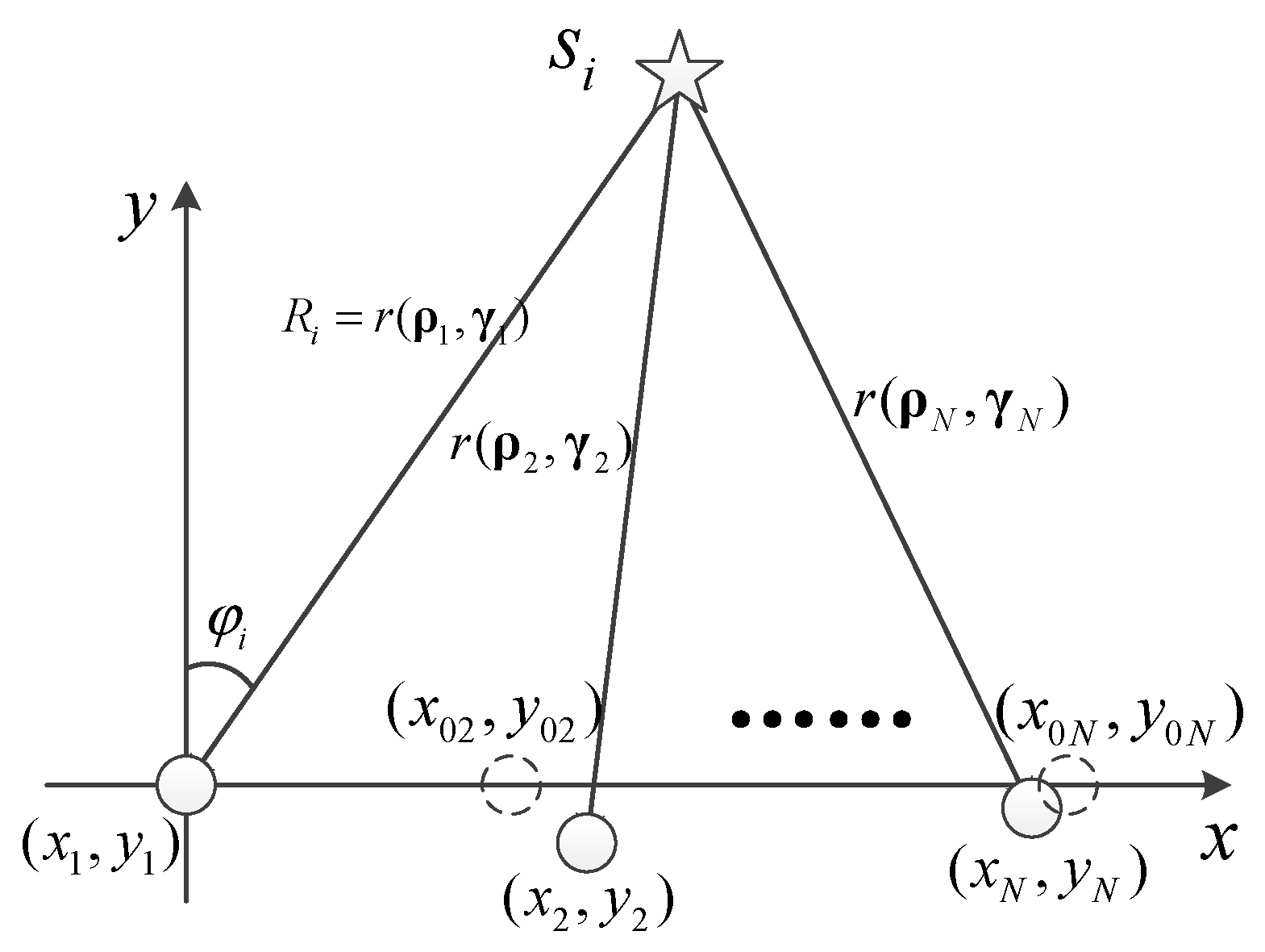
2. Error Model of Array Position with Near-Field Source

We consider the two-dimensional error model of arbitrary horizontal array that was used in the authors’ previous articles [12]. We suppose the number of elements is $N$, the number of near-field sources is $M$, and each source is an irrelevant narrow-band signal. The locations of sources are recorded as ${\mathit{\gamma }}_{\begin{array}{c}i\end{array}}=[{\phi }_i,R_i],i=1,2,\dots ,M$.

Most of the existing methods of element position estimation use the plane wave incidence model, which is suitable for the case that source locates in far field. That is, the distance $r$ between source and array satisfies $r>\mathsf{\pi }{D}^2/\lambda$, where $D$ denotes the maximum aperture of the array, and $\lambda$ denotes signal wavelength. When the space is limited, and the array aperture is large, the above conditions are difficult to be satisfied. At this time, the wave along the spherical wave is shown in Figure 1. We use the position of the first element as the origin to establish coordinate system. It means that, the first element is basic one, and its error is 0.

The received signal vector corresponding to the $i$th source can be modeled as:

$${\mathit{x}}_{ri}(t)={\mathit{A}}_i{s}_i(t)+\mathit{n}(t)\begin{array}{c}\end{array},\begin{array}{c}\end{array}i=1,2,\dots ,M.$$

(1)

where $s_i(t)$ is the signal emitted by the $i$th source, $\mathit{n}(t)$ is a complex Gaussian white noise matrix with zero mean, and ${\sigma }^2$ variance. In many applications, the assumption of white noise is not true, so the noise covariance matrix needs to be estimated in order to pre-whiten the noise. Without losing generality, we take the first hydrophone as the reference element (located at the origin of the coordinate and the position error is 0). If $\mathit{\rho }$ is used to denote the position of the array,

$$\begin{array}{l}\mathit{\rho }=[{\mathit{\rho }}_1,{\mathit{\rho }}_2,\dots ,{\mathit{\rho }}_N]\\ {\mathit{\rho }}_n={[x_n,y_n]}^T,\begin{array}{c}\end{array}n=1,2,\dots ,N\end{array}$$

(2)

$R_i$ denotes the distance between the $i$th source and origin, the array manifold ${\mathit{A}}_i$ can be expressed as:

$${\mathit{A}}_i=\left[\begin{array}{c}1\\ \frac{R_i}{r\left({\mathit{\rho }}_2,{\mathit{\gamma }}_i\right)}\exp [-\mathrm{j}\frac{2\mathsf{\pi }}{\lambda }(r\left({\mathit{\rho }}_2,{\mathit{\gamma }}_i\right)-R_i)]\\ ⋮\\ \frac{R_i}{r\left({\mathit{\rho }}_N,{\mathit{\gamma }}_i\right)}\exp [-\mathrm{j}\frac{2\mathsf{\pi }}{\lambda }(r\left({\mathit{\rho }}_N,{\mathit{\gamma }}_i\right)-R_i)]\end{array}\right],$$

(3)

where $r\left({\mathit{\rho }}_n,{\mathit{\gamma }}_i\right)$ is the distance between the $i$th source and the $n$th element,

$$r\left({\mathit{\rho }}_n,{\mathit{\gamma }}_i\right)=\sqrt{{(R_i\sin ({\phi }_i)-x_n)}^2+{(R_i\cos ({\phi }_i)-y_n)}^2}.$$

(4)

When the array has position errors,

$$\{\begin{array}{l}{x}_n=x_{0n}+\Delta x_n\\ y_n=y_{0n}+\Delta y_n\end{array}\begin{array}{c}\end{array},\begin{array}{c}\end{array}n=1,2,\dots ,N,$$

(5)

where $(x_{0n},y_{0n})$ represents the nominal position of the array element, $(\Delta x_n,\Delta y_n)$ is the position error of the element, $\Delta x_1=\Delta y_1=0$ and $x_1=y_1=0$.

For the far-field problem, the steering vector can be simplified to a linear function by logarithm operation, but the near-field steering vector is a complex nonlinear function.

When we know the sources’ position, the array manifold is a nonlinear function of the element position errors. As shown in Equation (3), there are $M(N-1)$ independent delays that can be measured, and $2(N-1)$ unknown values about element positions. In order to get a unique solution, when $N\ge 2$, the number of auxiliary sources needs to satisfy $M\ge 2$.

When the sources positions are unknown, in order to find the baseline basis for the array calibration, we set $\Delta x_1=\Delta y_1=\Delta y_2=0$, so that the steering vector is a nonlinear function of the element position errors and the sources’ position. This model has $M(N-1)$ independent equations, where existences $2N-3$ element position errors and $2M$ sources’ position are unknown values (considering the two-dimensional source position). In order to obtain a unique solution, when $N\ge 4$, the number of sources needs to satisfy $M\ge \frac{2N-3}{N-3}$, otherwise $N\le 3$, there is no solution.

3. Methods

3.1. Near-Field Element Position Calibration Based on Maximum Likelihood Estimation

An effective way to solve the nonlinear function problem of near-field steering vector is to use the optimal solution algorithm. This method does not need to approximate the nonlinear function, and theoretically can achieve CRLB. Based on this idea, using unconditional maximum likelihood estimator (UML) [23], this paper proposes a near-field geometry calibration method. This method can not only be used for auxiliary calibration, separately estimating the positions of the elements, but also be used for self-calibration, achieving a joint estimation of elements’ positions and sources’ position. It can even be used under the conditions that partial sources’ positions are known. This paper mainly discusses the auxiliary calibration and self-calibration based on maximum likelihood estimation, and abbreviates them as “ML-GC” and “ML-GAC” respectively.

We set $\mathit{S}$ as the sample function of Gaussian random process, its spectral matrix is unknown, additive noise is spatially uncorrelated Gaussian noise, and its spectrum is ${\mathit{R}}_n$. The number of snapshots is indicated by a corner mark. If there are $M$ independent near-field sources with different positions, the received samples $\mathit{X}$ can be expressed as:

$$\begin{array}{l}{\mathit{X}}_k=\mathit{A}\left(\mathit{\alpha }\right){\mathit{S}}_k+{\mathit{N}}_k\\ \mathit{A}\left(\mathit{\alpha }\right)=\left[{\mathit{A}}_1\left(\mathit{\alpha }\right),{\mathit{A}}_2\left(\mathit{\alpha }\right),\dots ,{\mathit{A}}_M\left(\mathit{\alpha }\right)\right]\\ {\mathit{S}}_k={\left[s_1{}_k,s_2{}_k,\dots ,s_M{}_k\right]}^{\mathrm{T}}\end{array}$$

(6)

where ${\mathit{A}}_i,i=1,\dots ,M$ as shown in the Formula (3), signals’ spectrum is ${\mathit{R}}_s=E\left[{\mathit{S}}_k{\mathit{S}}_k{}^H\right]$, and $\mathit{\alpha }$ is unknown vector.

We assume that

$${\mathit{R}}_n={\sigma }_n^2\mathit{I},$$

(7)

and ${\sigma }_n^2$ is unknown. The likelihood function can be expressed as

$$L\left(\mathit{\alpha },{\mathit{R}}_s,{\sigma }_n^2\right)=-\ln \det {\mathit{R}}_x-\frac{1}{K}{\displaystyle \sum _{k=1}^K{\mathit{X}}_k^H{\mathit{R}}_x^{-1}{\mathit{X}}_k},$$

(8)

where $K$ denotes the number of snapshots, and

$${\mathit{R}}_x=\mathit{A}\left(\mathit{\alpha }\right){\mathit{R}}_s{\mathit{A}}^H\left(\mathit{\alpha }\right)+{\sigma }_n^2\mathit{I}.$$

(9)

We use ${\mathit{C}}_x$ to denote the sampling correlation matrix, then

$${\mathit{C}}_x=\frac{1}{K}{\displaystyle \sum _{k=1}^K{\mathit{X}}_k{\mathit{X}}_k^H}.$$

(10)

The likelihood function can be expressed as

$$L\left(\mathit{\alpha },{\mathit{R}}_s,{\sigma }_n^2\right)=-\left[\ln \det {\mathit{R}}_x+\mathrm{tr}\left({\mathit{R}}_x^{-1}{\mathit{C}}_x\right)\right].$$

(11)

For the above formula, we first maximize it on ${\mathit{R}}_x$ to get the equation of unknown vector $\mathit{\alpha }$, and then find the maximum value of the equation, so as to get all the solutions.

Let $R_{i,j}$ be the element in ${\mathit{R}}_s$, then ${\mathit{R}}_x$ can be expressed as

$${\mathit{R}}_x={\displaystyle \sum _{i=1}^M{\displaystyle \sum _{j=1}^M{R}_{i,j}\mathit{A}\left({\mathit{\alpha }}_i\right){\mathit{A}}^H\left({\mathit{\alpha }}_j\right)}}+{\sigma }_n^2\mathit{I}.$$

(12)

According to the necessary conditions

$$\frac{\partial L\left(\mathit{\alpha },{\mathit{R}}_s,{\sigma }_n^2\right)}{\partial R_{i,j}}=0,\begin{array}{cc}& \end{array}i,j=1,2,\dots ,M,$$

(13)

$$\frac{\partial L\left(\mathit{\alpha },{\mathit{R}}_s,{\sigma }_n^2\right)}{\partial {\sigma }_n^2}=0$$

(14)

.

The solutions of ${\mathit{R}}_x$ and ${\sigma }_n^2$ in the above formula can be obtained, which are denoted as ${\widehat{\mathit{R}}}_x$ and ${\widehat{\sigma }}_n^2$:

$${\widehat{\mathit{R}}}_x\left(\mathit{\alpha }\right)={\mathit{P}}_A\left({\mathit{C}}_x-{\sigma }_n^2\mathit{I}\right){\mathit{P}}_A+{\sigma }_n^2\mathit{I},$$

(15)

$${\widehat{\sigma }}_n^2=\frac{\mathrm{tr}\left[{\mathit{P}}_A^{\perp }{\mathit{C}}_x\right]}{N-M}.$$

(16)

${\mathit{P}}_A$ is the projection matrix of the steering vector $\mathit{A}$, and ${\mathit{P}}_A^{\perp }$ is the orthogonal component of ${\mathit{P}}_A$:

$${\mathit{P}}_A=\mathit{A}{({\mathit{A}}^H\mathit{A})}^{-1}{\mathit{A}}^H,$$

(17)

$${\mathit{P}}_A^{\perp }=\mathit{I}-{\mathit{P}}_A.$$

(18)

Next ${\mathit{R}}_x$ in Formula (11) is replaced by ${\widehat{\mathit{R}}}_x$, and the maximum value of Formula (11) is solved. We take $\widehat{\mathit{\alpha }}$ as the estimation of $\mathit{\alpha }$, then

$$\widehat{\mathit{\alpha }}=\arg \underset{\mathit{\alpha }}{\max }\left\{-\ln \det \left[{\mathit{P}}_A{\mathit{C}}_x{\mathit{P}}_A+\frac{\mathrm{tr}({\mathit{P}}_A^{\perp }{\mathit{C}}_x){\mathit{P}}_A^{\perp }}{N-M}\right]\right\},$$

(19)

$$\begin{array}{c}\widehat{\mathit{\alpha }}=\end{array}=\arg \underset{\mathit{\alpha }}{\min }\left\{\det \left[{\mathit{P}}_A{\mathit{C}}_x{\mathit{P}}_A+\frac{\mathrm{tr}({\mathit{P}}_A^{\perp }{\mathit{C}}_x){\mathit{P}}_A^{\perp }}{N-M}\right]\right\},N\ne M.$$

(20)

The above formula is the UML. Define unknown vector $\mathit{\alpha }$ according to different array calibration methods. The unknown vector $\mathit{\alpha }$ in the auxiliary calibration method only contains the position error of the array, and $\mathit{\alpha }={\left[\Delta x,\Delta y\right]}^T$, $\Delta x_1=\Delta y_1=0$. It also includes the target position parameter in the self-calibration method, that is $\mathit{\alpha }={\left[\mathit{R},\mathit{\phi },\Delta x,\Delta y\right]}^{\mathrm{T}}$. In order to obtain a baseline, we set $\Delta x_1=\Delta y_1=\Delta y_2=0$.

The optimization algorithm such as differential evolution algorithm (DE) or Levenberg-Marquardt algorithm (LM) [24,25] can be used to solve the Problem (20) to obtain the unknown parameter vector. In the later simulation, we use the DE to solve the above optimization problem. Its characteristic is that it uses the local information of individual and the global information of the group to search together, and has strong universality. It can be directly applied to auxiliary calibration and self-calibration without changing the basic model of the algorithm. Its calculation process is simple, but the amount of computation of this kind of evolutionary algorithms is a little large.

The optimization problem can be expressed as:

$$\begin{array}{l}\min F(\mathit{\alpha })=\det \left[{\mathit{P}}_A{\mathit{C}}_x{\mathit{P}}_A+\frac{\mathrm{tr}({\mathit{P}}_A^{\perp }{\mathit{C}}_x){\mathit{P}}_A^{\perp }}{N-M}\right],N\ne M\begin{array}{c},\end{array}\mathit{\alpha }={\left[\Delta x,\Delta y\right]}^T\begin{array}{c}\end{array}or\begin{array}{c}\end{array}\mathit{\alpha }={\left[\mathit{R},\mathit{\phi },\Delta x,\Delta y\right]}^{\mathrm{T}}\\ s.t.\begin{array}{c}\end{array}{\alpha }_i\in \left[l_i,u_i\right]\end{array}$$

(21)

where ${\alpha }_i$ is the $i$th element in $\mathit{\alpha }$, and $\left[l_i,u_i\right]$ is its value range. It includes four steps to solve the problem by DE, and they are population initialization, variation, crossing, and selection. In this paper, we use DE/best/1/bin to solve Formula (21), and take the self-calibration method as an example:

Step 1, population initialization. Each individual in the population represents a solution to the optimization problem. We set that the population size is $U$ = 300, the $k$th individual is ${\mathit{\alpha }}_k=[{\alpha }_{1,k},{\alpha }_{2,k},{\alpha }_{3,k},{\alpha }_{4,k}]$, and achieve the first generation like this:

$${\alpha }_{i,k}(0)=l_i+\mathrm{rand}\cdot (u_i-l_i),\begin{array}{c}\end{array}k=1,\dots ,U,$$

(22)

where $\mathrm{rand}\in$[0,1], it is random numbers that follow a uniform distribution. The range of $\mathit{R}$ covers the whole near field. The direction of arrival $\mathit{\phi }$ ranges from −90° to 90°. The errors $\Delta x$ and $\Delta y$ range from $-d/2$ to $d/2$, where $d$ is the element space.

Step 2, DE/best/1 variation. Generate a target individual $t_k(g)$ for each individual ${\mathit{\alpha }}_k(g)$ in the current population, where $g$ is the evolution generation,

$${\mathit{t}}_k(g)={\alpha }_{best}(g)+Q\left[{\mathit{\alpha }}_{u1}(g)-{\mathit{\alpha }}_{u2}(g)\right].$$

(23)

where $u_1,u_2\in \{1,2,\cdots ,U\}\&u_1,u_2\ne k$, ${\mathit{\alpha }}_{best}(g)$ is the best individual of the $g$th generation, and taken as variation operation base. $Q\in [0,1)$ is the zoom factor, and we set $Q=0.85$.

Step 3, binomial crossing (DE/best/1/bin). Generate an equally distributed random number ${\gamma }_{i,k}\in \left[0,1\right]$ for every variable of each individual, complete crossing operation, and generate test individual $v_k(g)$:

$$v_{i,k}(g)=\{\begin{array}{l}{t}_{i,k}(g),\begin{array}{c}\end{array}{\gamma }_{i,k}<cr\\ {\alpha }_{i,k}(g),\begin{array}{c}\end{array}else\end{array},$$

(24)

where threshold $cr\in \left[0,1\right]$, we choose $cr=1$. It means that we use $t_k(g)$ as the test individual primarily.

Step 4, greedy selection. Select the better individual to go to the next generation.

$${\mathit{\alpha }}_k(g+1)=\{\begin{array}{l}{\mathit{t}}_k(g),\begin{array}{c}\end{array}F({\mathit{t}}_k(g))<F({\mathit{\alpha }}_k(g))\\ {\mathit{\alpha }}_k(g),\begin{array}{c}\end{array}else\end{array},$$

(25)

Iteration termination condition: Objective function $F({\mathit{\alpha }}_k(g))$ is smaller than termination threshold, or the times of iteration is large enough. In this paper, the max times of iteration is 500, there is no termination threshold of objective function, and then we get the final estimation.

The computation of this method is mainly decided by the population size $U$, the number of variables, and times of iterations. First, we calculate the data covariance matrix, and just do it once, as it is small amount of calculation. Its amount of calculation is $N\times K$ dimension matrix multiplication. Second, population initialization, we randomly generate $H\times U$ dimension matrix, where $H$ is the length of $\mathit{\alpha }$. Variation, crossing, and selection are all based on this dimension matrix to complete some simple logic and numerical operations. This process is repeated 500 times.

3.2. Multipath Compensation Method

Considering the underwater correlated multipath environment, the steering vector becomes

$$\tilde{\mathit{A}}=\left[{\tilde{\mathit{A}}}_1,{\tilde{\mathit{A}}}_2,\dots ,{\tilde{\mathit{A}}}_M\right],$$

(26)

where ${\tilde{\mathit{A}}}_i,i=1,\dots ,M$ is

$${\tilde{\mathit{A}}}_i(\Delta \mathit{x},\Delta \mathit{y})={\mathit{A}}_i(\Delta \mathit{x},\Delta \mathit{y})+{\displaystyle \sum _l\mathit{A}{\mathit{r}}_{li}(\Delta \mathit{x},\Delta \mathit{y})},$$

(27)

and $\mathit{A}{\mathit{r}}_{li}(\Delta \mathit{x},\Delta \mathit{y})$ represents the steering vector corresponding to the $l$th reflection path

$$\mathit{A}{\mathit{r}}_{li}(\Delta \mathit{x},\Delta \mathit{y})=\left[\begin{array}{c}{f}_{1i}^l\\ f_{2i}^l\\ \begin{array}{c}\end{array}⋮\\ f_{Ni}^l\end{array}\right]\otimes \left[\begin{array}{c}\frac{R_i}{r_{1i}^l\left(\Delta \mathit{x},\Delta \mathit{y}\right)}\exp [-\mathrm{j}\frac{2\mathsf{\pi }}{\lambda }(r_{1i}^l\left(\Delta \mathit{x},\Delta \mathit{y}\right)-R_i)]\\ \frac{R_i}{r_{2i}^l\left(\Delta \mathit{x},\Delta \mathit{y}\right)}\exp [-\mathrm{j}\frac{2\mathsf{\pi }}{\lambda }(r_{2i}^l\left(\Delta \mathit{x},\Delta \mathit{y}\right)-R_i)]\\ ⋮\\ \frac{R_i}{r_{Ni}^l\left(\Delta \mathit{x},\Delta \mathit{y}\right)}\exp [-\mathrm{j}\frac{2\mathsf{\pi }}{\lambda }(r_{Ni}^l\left(\Delta \mathit{x},\Delta \mathit{y}\right)-R_i)]\end{array}\right].$$

(28)

The “$\otimes$” indicates the multiplication of the corresponding items. $f_{ni}^l$ and $r_{ni}^l\left(\Delta \mathit{x},\Delta \mathit{y}\right)$ respectively represent the reflection coefficient and the sound path. The corner marks $n$, $i$, $l$ respectively represent the $n$th element, the $i$th source, and the $l$th reflection path. The sound path can be described as

$$r_{ni}^l\left(\Delta \mathit{x},\Delta \mathit{y}\right)=\sqrt{{(R_i\sin ({\theta }_i)\sin ({\phi }_i)-x_n)}^2+{(R_i\sin ({\theta }_i)\cos ({\phi }_i)-y_n)}^2+{(z^l-z_n)}^2},$$

(29)

where $z^l$ is the equivalent virtual source depth, ${\phi }_i$ is the pitch angle of the real sources. The received signal is equivalent to

$${\tilde{\mathit{X}}}_k=\tilde{\mathit{A}}\left(\mathit{\alpha }\right){\mathit{S}}_k+{\mathit{N}}_k,$$

(30)

We use $\tilde{\mathit{A}}$ to replace $\mathit{A}$ in Equation (6). The reflection coefficients can be achieved by the channel estimation algorithm [26], and then we can obtain the novel near-field calibration method based on maximum likelihood matching. It is suitable for strong multipath environment. Especially for the auxiliary calibration, multipath structure and reflection coefficients can be estimated with high accuracy. For the self-calibration with unknown source, multipath can also be estimated, but the accuracy is affected. This paper mainly analyzes the multipath problem in the auxiliary calibration. For the self-calibration method, the model is still valid, but the specific research will be expanded in the follow-up research. The corresponding auxiliary calibration is recorded as “MLM-GC.”

4. Simulation and Experiment

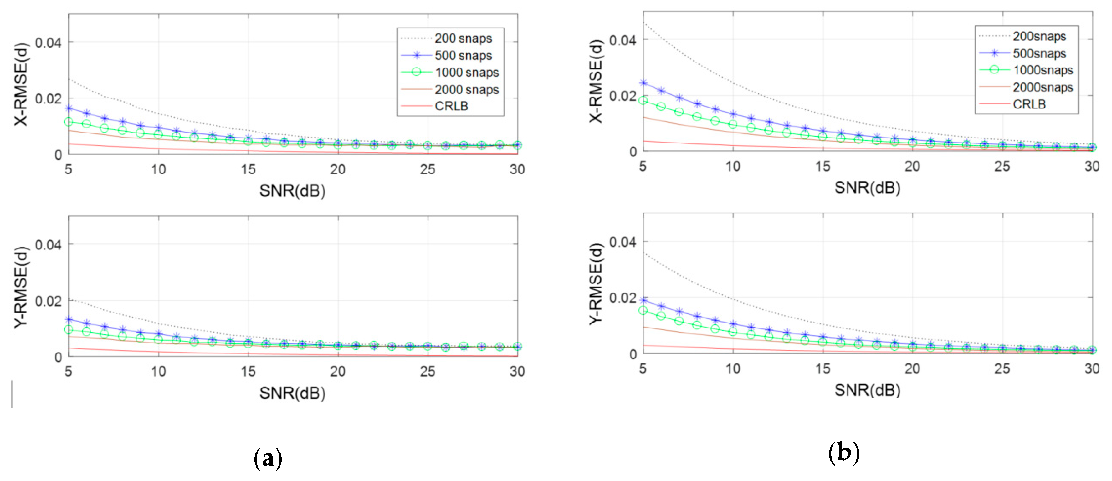
4.1. Simulation

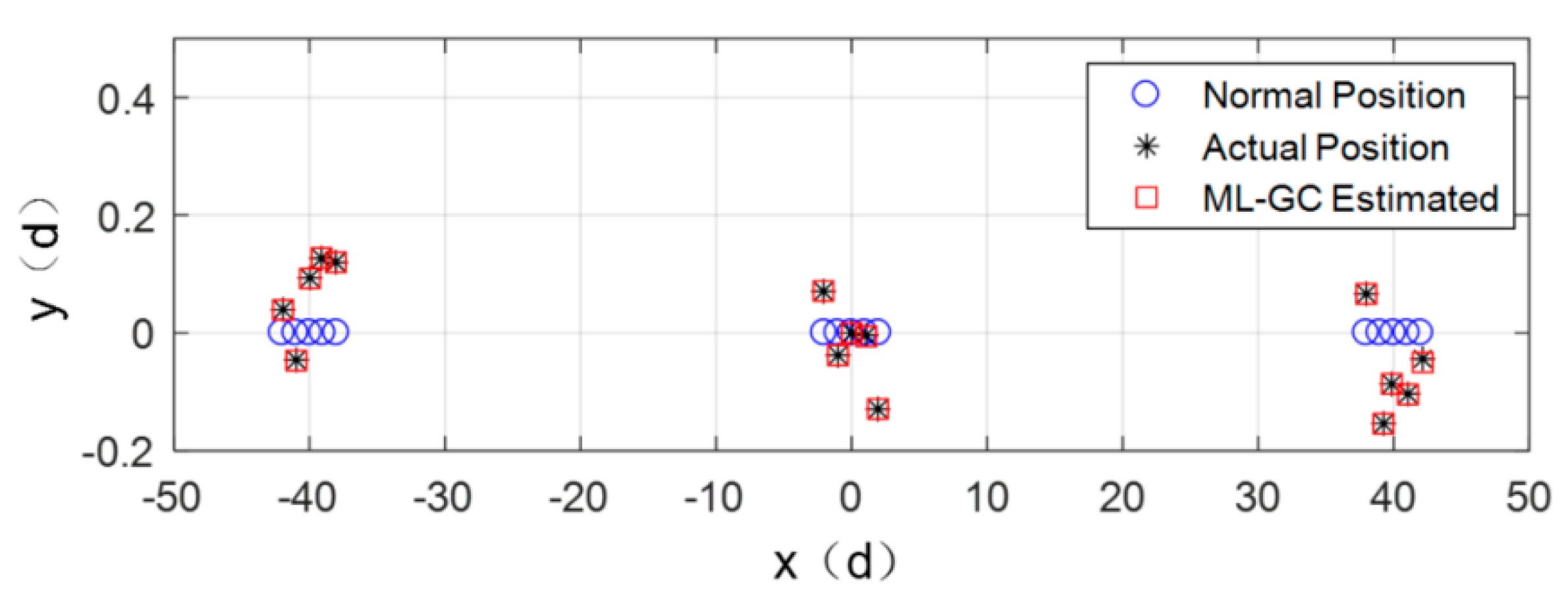
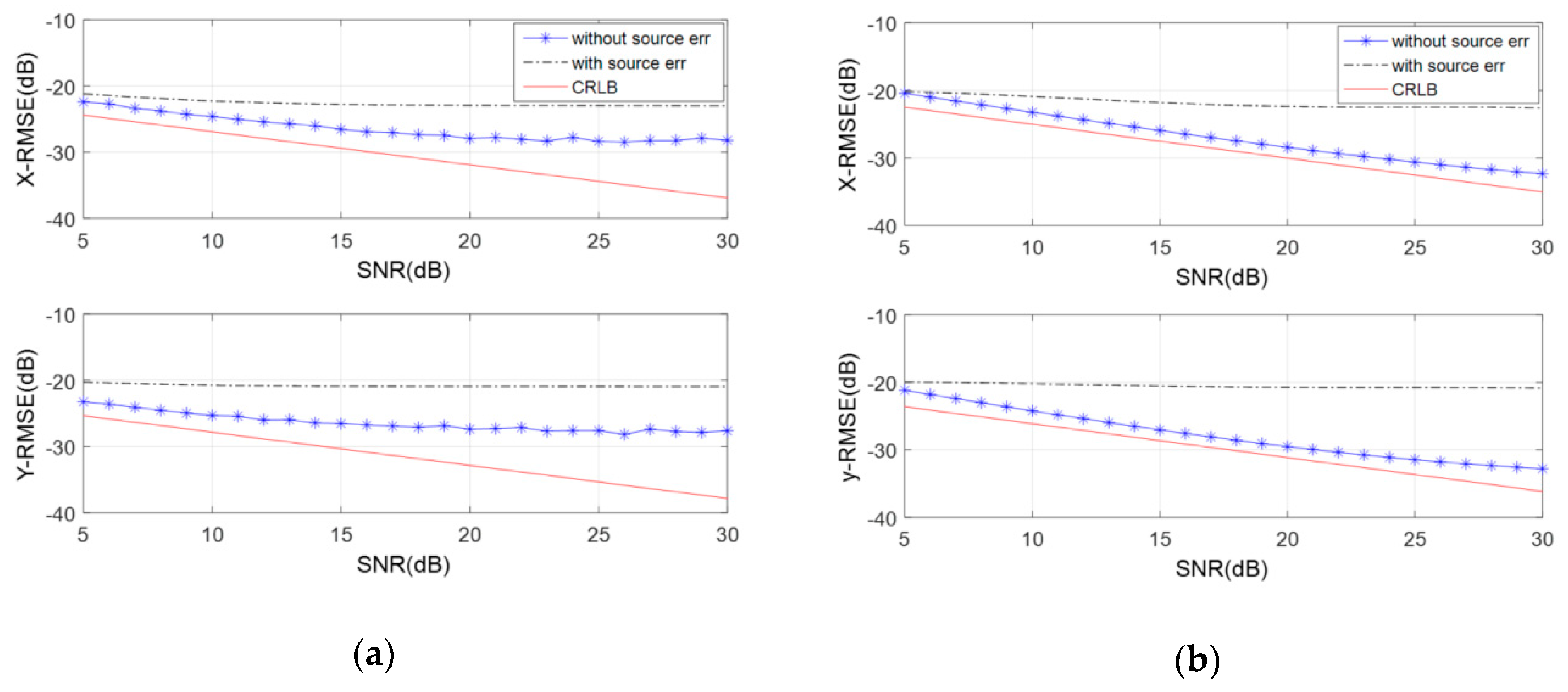
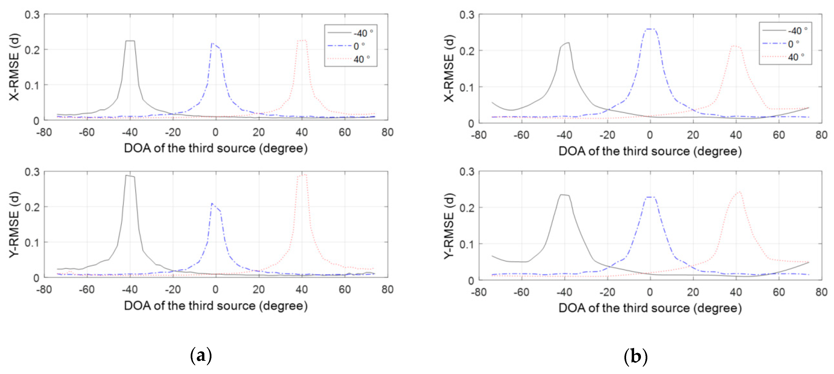
4.1.1. Near-field Auxiliary Calibration Method Base on Maximum Likelihood Estimation (ML-GC)

In this section, we use a 15-element long linear array as an example to simulate and analyze the performance of ML-GC. We divide the array into three 5-element sub-arrays. The distance between each sub-array is 20 m. The subarray space $d=\lambda /2=0.5\begin{array}{c}\end{array}\mathrm{m}$, $\lambda$ is signal wavelength, and SNR = 20 dB. We set array center as coordinate origin, and randomly generate a two-dimensional array error with standard deviation $0.1$ d. The two auxiliary sources’ DOAs are −30° and 40°. The distance from each source to the origin is both 20 m. We use 1000 snapshots.

Figure 2 shows the simulation result. The circles in the figure represent the nominal positions of elements, the asterisks are their actual positions, and the squares are the elements’ positions estimated by ML-GC. It can be seen that ML-GC proposed in this paper can achieve the real element position, which verifies its effectiveness with near field source.

Table 1. Array shape estimation.

Element Num.	Nominal Position (d)		Actual Position (d)		ML−GC(d)		Absolute Error(d)
	X	Y	X	Y	X	Y	X	Y
1	−42.000	0.000	−41.952	0.040	−41.954	0.048	0.002	0.008
2	−41.000	0.000	−40.975	0.046	−40.970	−0.047	0.005	0.001
3	−40.000	0.000	−39.967	0.094	−39.967	0.095	0.000	0.001
4	−39.000	0.000	−39.112	0.127	−39.114	0.130	0.002	0.003
5	−38.000	0.000	−38.061	0.120	−38.063	0.123	0.002	0.003
6	−2.000	0.000	−2.078	0.071	−2.078	0.072	0.000	0.001
7	−1.000	0.000	−1.005	−0.038	−1.006	−0.035	0.001	0.003
8	0.000	0.000	0.000	0.000	0.000	0.000	0.000	0.000
9	1.000	0.000	1.079	−0.004	1.079	−0.003	0.000	0.001
10	2.000	0.000	1.943	−0.129	1.941	−0.127	0.002	0.002
11	38.000	0.000	37.977	0.067	37.970	0.065	0.007	0.002
12	39.000	0.000	39.257	−0.154	39.257	−0.153	0.000	0.001
13	40.000	0.000	39.861	−0.087	39.863	−0.085	0.002	0.002
14	41.000	0.000	41.052	−0.104	41.046	−0.107	0.006	0.003
15	42.000	0.000	42.139	−0.044	42.135	−0.046	0.004	0.002

shows the estimation results and accuracy of elements’ positions. The estimation errors in the X-axis is smaller than 0.006 d, in the Y-axis is smaller than 0.008 d.

Here we use a near-field focusing beam forming result to observe the effect of our calibration. We suppose that there are two targets in the near field, and they locate at (−70.71 m, 70.71 m) and (76.60 m, 64.28 m), SNR = 20 dB. Figure 3 shows the spatial spectral results.

As shown in Figure 3, with geometry errors of array, two targets’ location errors are (−1.41, 1.41) and (−3.06, −2.57). After calibration by ML-GC, the location errors reduce to (0, 0) and (0, 0). For near field targets, the spatial spectrum is seriously affected by the array geometry errors, and the positioning accuracy is reduced, especially the range accuracy. After calibration using ML-GC, the near-field positioning accuracy has been improved and is basically the same as that of using the actual elements positions. It fully illustrates that array calibration can weaken the impact caused by the array geometry errors.

The simulation conditions are the same as above. The following is compared with the eigenvector method (EV-GC) which is a kind of classical near field calibration method to study the estimation accuracy change with spectrum level SNR, snapshot, and source position. EV-GC uses the relationship between steering vector and signal eigen vector to establish equation. Then it uses Taylor approximation to change the non-linear equation to a linear one. So we can solve for the analytic solution of the unknown values [12]. Here we use 200 Monte Carlo simulations. Here we calculate its RMSE like this:

$$\begin{array}{l}RMS{E}_X=\frac{1}{M_C(N-1)}{\displaystyle \sum _{l=1}^{M_c}{\displaystyle \sum _{n=2}^N{({\widehat{x}}_{n,l}-x_{n,l})}^2}}\\ RMS{E}_Y=\frac{1}{M_C(N-1)}{\displaystyle \sum _{l=1}^{M_c}{\displaystyle \sum _{n=2}^N{({\widehat{y}}_{n,l}-y_{n,l})}^2}}\end{array}$$

(31)

$\left({\widehat{x}}_{n,l},{\widehat{y}}_{n,l}\right)$ is the estimated result of the $n$th element, the $l$th time of Monte Carlo simulations. $\left(x_{n,l},y_{n,l}\right)$ is its real value. RMSE unit is “d” in Figure 4, and its element space. So the values shown in Figure 4 are the result of $RMS{E}_X$ and $RMS{E}_Y$ divided by d.

Figure 4 shows the estimation RMSE of geometry errors with SNR increasing under different numbers of snapshots using EV-GC and ML-GC. In general, all errors decrease with the increase of the snapshots number or SNR. The main reason is that EV-GC and ML-GC use the received data covariance matrix as the estimation of array covariance matrix, and the effect of this estimation depends on the snapshots number and SNR. When the SNR is high, the required snapshots number can be significantly reduced.

When the spectrum level SNR is greater than 25 dB, the RMSE of EV-GC tends to be stable gradually, and the estimation accuracy no longer changes with SNR. The reason is that the statistical estimation error is dominant when the SNR is less than 25 dB, while the calibration error of EV-GC is dominated by model approximation error when SNR is greater than 25 dB. In order to solve a nonlinear function, EV-GC uses a model approximation method.

The estimation accuracy of EV-GC is higher than that of ML-GC at low SNR, which indicates that ML-GC has higher requirements for SNR than EV-GC. When SNR is higher than 25 dB, ML-GC has higher estimation accuracy than EV-GC because ML-GC does not introduce model approximation, and the estimation accuracy of ML-GC gradually approaches CRLB as the SNR increases. It is worth noting that the SNR is usually higher than 25 dB in the near-field calibration scene, and at this time ML-GC is better than EV-GC in terms of accuracy. In addition, ML-GC is unbiased estimation.

Next, we introduce the position errors of auxiliary sources. We set the errors of source positions obey the Gauss distribution with mean value 0, standard deviation 0.01 rad and 1 cm. Figure 5 shows the comparison of estimation errors with and without source errors using 1000 snapshots and 500 Monte Carlo experiments. In order to show the details, we show X-RMSE and Y-RMSE in the unit “dB” like this:

$$\begin{array}{l}RMS{E}_X=10\lg \left\{\left[\frac{1}{M_C(N-1)}{\displaystyle \sum _{l=1}^{M_c}{\displaystyle \sum _{n=2}^N{({\widehat{x}}_{n,l}-x_{n,l})}^2}}\right]/d\right\}\\ RMS{E}_Y=10\lg \left\{\left[\frac{1}{M_C(N-1)}{\displaystyle \sum _{l=1}^{M_c}{\displaystyle \sum _{n=2}^N{({\widehat{y}}_{n,l}-y_{n,l})}^2}}\right]/d\right\}\end{array}$$

(32)

When there is no source error, ML-GC is closer to CRLB than EV-GC. When there is no source error and SNR is higher than 17 dB, the ML-GC has higher estimation accuracy than EV-GC. When there are source errors, the two methods are still effective, but the errors increase. The influence of source error is stronger than that of statistical estimation error in high SNR. Figure 5 shows that the proposed method ML-GC has a certain tolerance for source error.

Next, we analyze the RMSE change of the array element position estimation with the azimuth of the two auxiliary sources. We fix one source at −40°, 0°, or 40°. The other one source changes from −75° to 75°. We use 100 snapshots, and have 100 Monte Carlo experiments. The results are shown in Figure 6.

As shown in Figure 6, when the orientations of the two auxiliary sources coincide, the position of the elements is unmeasurable, and the estimation error tends to infinity. When the angle between the two auxiliary sources is less than 20°, RMSEs are higher than 0.05 d, and the estimation error of the element position decreases sharply with the increase of their included angle. The performance tends to be stable when it is greater than 20°. EV-GC and ML-GC have similar conclusions. In order to ensure the performance of the algorithm, the included angle of the two auxiliary sources should be greater than 20° and the auxiliary source should be away from the axial direction of the line array.

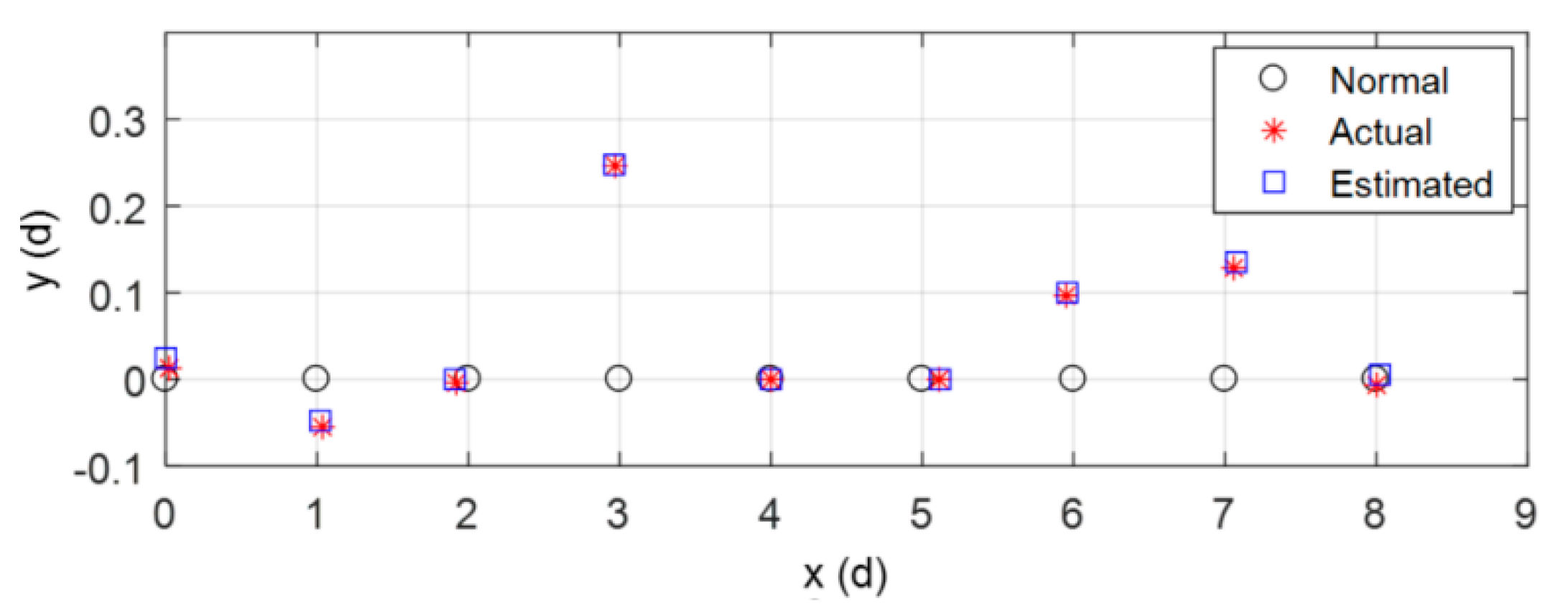
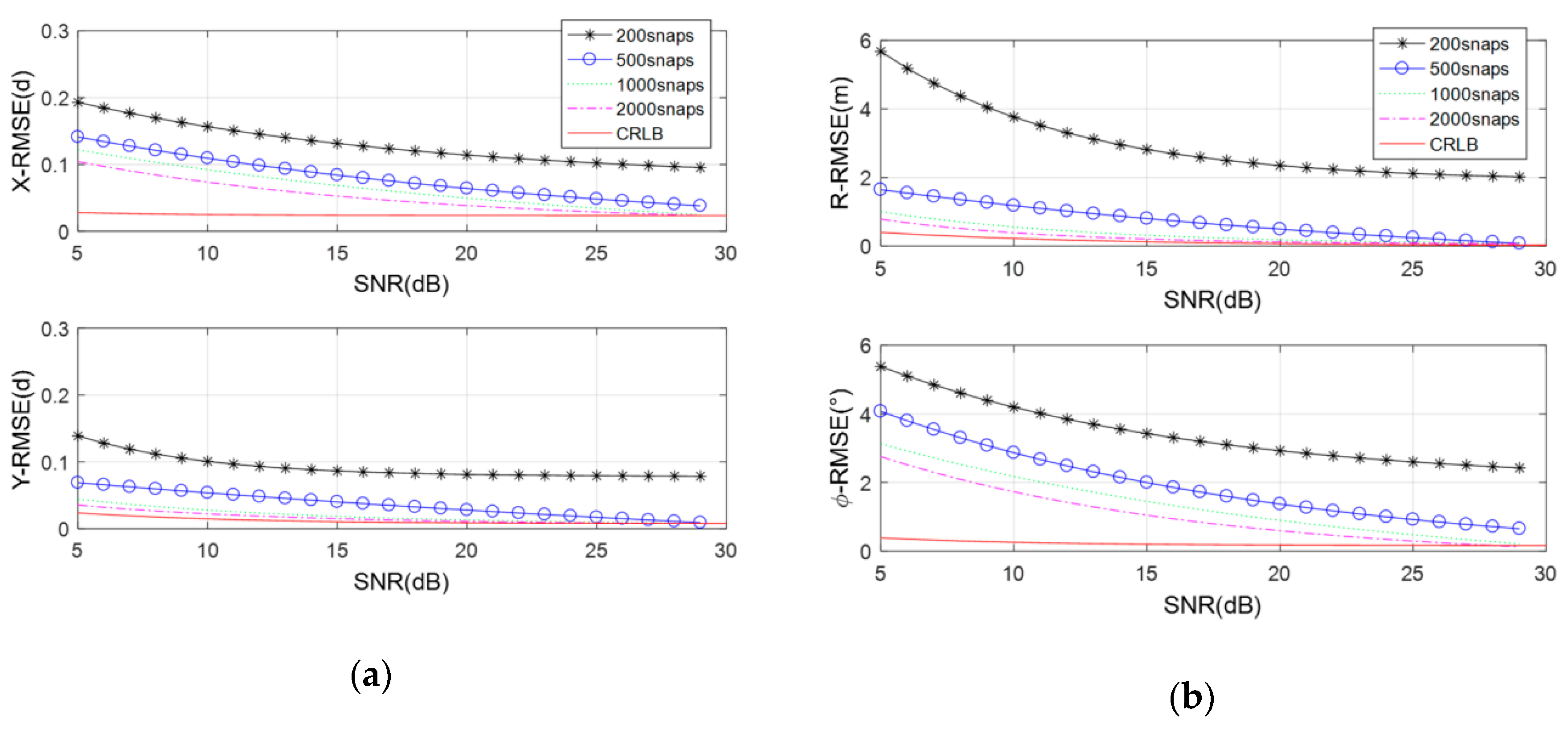
4.1.2. Near-Field Self-Calibration Method Based on Maximum Likelihood Estimation (ML-GAC)

First we verify the effectiveness of the ML-GAC proposed in this paper. We take the 9-element line array as an example, and assume that the array element spacing is $d=\lambda /2=0.5$ m, the SNR is 20 dB, and the elements position errors are randomly generated with a standard deviation of 0.1 d, mean value of 0. Only horizontal two-dimensional elements position errors are considered. The three targets’ DOAs are −60°, 0°, 40°. The distance between each source and the first element is 10 m. We simulate with 1000 snapshots.

Figure 7,

Table 2. Calibration result of ML-GAC.

Element Num.	Nominal Position (d)		Actual Position (d)		ML−GAC (d)		Absolute Error (d)
	X	Y	X	Y	X	Y	X	Y
1	0	0	0.180	−0.078	0.195	−0.078	0.015	0.000
2	1	0	1.037	−0.117	1.050	−0.117	0.013	0.000
3	2	0	1.887	0.084	1.894	0.086	0.007	0.002
4	3	0	2.813	0.151	2.812	0.151	0.001	0.000
5	4	0	4.000	0.000	4.000	0.000	0.000	0.000
6	5	0	4.985	0.000	4.979	0.000	0.006	0.000
7	6	0	5.928	0.191	5.916	0.191	0.012	0.000
8	7	0	7.093	−0.040	7.087	−0.035	0.006	0.005
9	8	0	7.996	−0.159	7.982	−0.153	0.014	0.006

and

Table 3. Target location results of ML-GAC.

Source Num.	Actual Distance (m)	Estimated Distance (m)	Absolute Error of Distance(m)	Actual DOA (Degree)	Estimated DOA (Degree)	Absolute Error of DOA (Degree)
1	10	9.9912	0.0088	−60	−60.5811	0.5811
2	10	9.8115	0.1885	0	0.1484	0.1484
3	10	9.7834	0.2166	40	40.3403	0.3403

show the calibration results and estimated sources locations using ML-GAC. They can verify its effectiveness. The estimation errors of array in the X-axis is smaller than 0.015 d, in the Y-axis is smaller than 0.006 d. The estimation errors of targets in distance is smaller than 0.2166°, in DOA is smaller than 0.5811°.

Based on the above simulation, this paper studies the estimation RMSE of ML-GAC changing with the spectrum level SNR, the number of snapshots and the position of the calibration sources.

We have 200 Monte Carlo experiments. Figure 8 shows the estimation RMSE of the array geometry errors and sources positions changing with SNR and snapshots number. It can be seen that the RMSE decreases as the number of snapshots or SNR increases. It is the same with ML-GC, and snapshots number and SNR affect the estimation accuracy of the signal covariance matrix. When the SNR is high and the number of snapshots is large, the algorithm accuracy is close to CRLB. Since the self-calibration method does not need to know the positions of the sources in advance, it is not affected by the position error of the sources, and the operation is relatively simple. However, since the variable dimension is increased, more sources are needed, and the estimation accuracy of the self-calibration method is lower than that of the auxiliary method. When SNR = 5 dB and we use 2000 snaps, the X-RMSE = 0.104 d, Y-RMSE = 0.035 d, R-RMSE = 0.787 m, $\varphi$-RMSE = 2.756°. When SNR = 20 dB and we use 2000 snaps, the X-RMSE = 0.039 d, Y-RMSE = 0.011 d, R-RMSE = 0.123 m, $\varphi$-RMSE = 0.595°.

Three sources are used, in which the two sources orientations are fixed at 0°and 40°and the third source orientation is changed from −75°to 75°. We have 1000 snapshots and 200 times of Monte Carlo experiments. Other conditions are the same as above. Figure 9 shows the RMSE of the elements and the sources position estimation changing with the target azimuth based on ML-GAC.

It can be seen from Figure 7 that when the third source position coincides with the other two sources, the estimation errors of the elements positions and the sources positions tend to infinity. The larger the angle between the third source and the other two sources, the higher the estimation accuracy. Therefore, in practical applications, the angle between the three sources should be as large as possible to ensure the estimated accuracy.

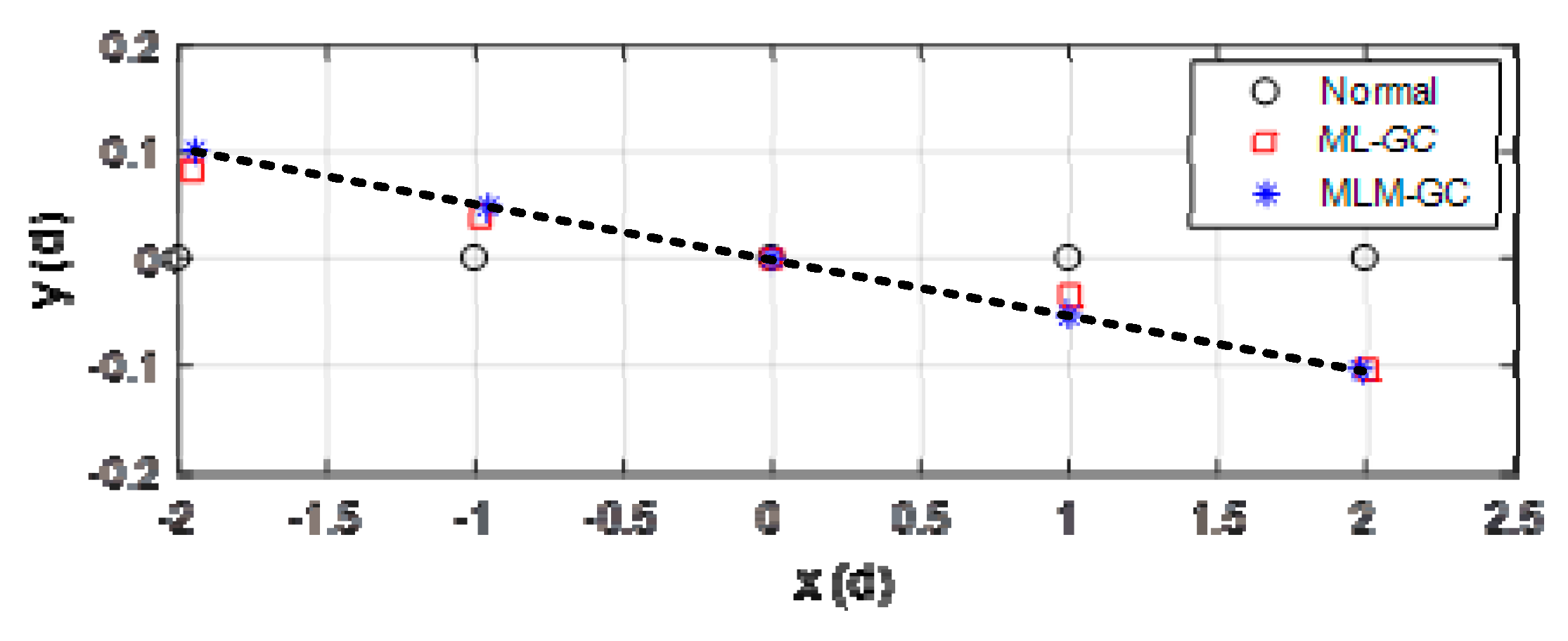
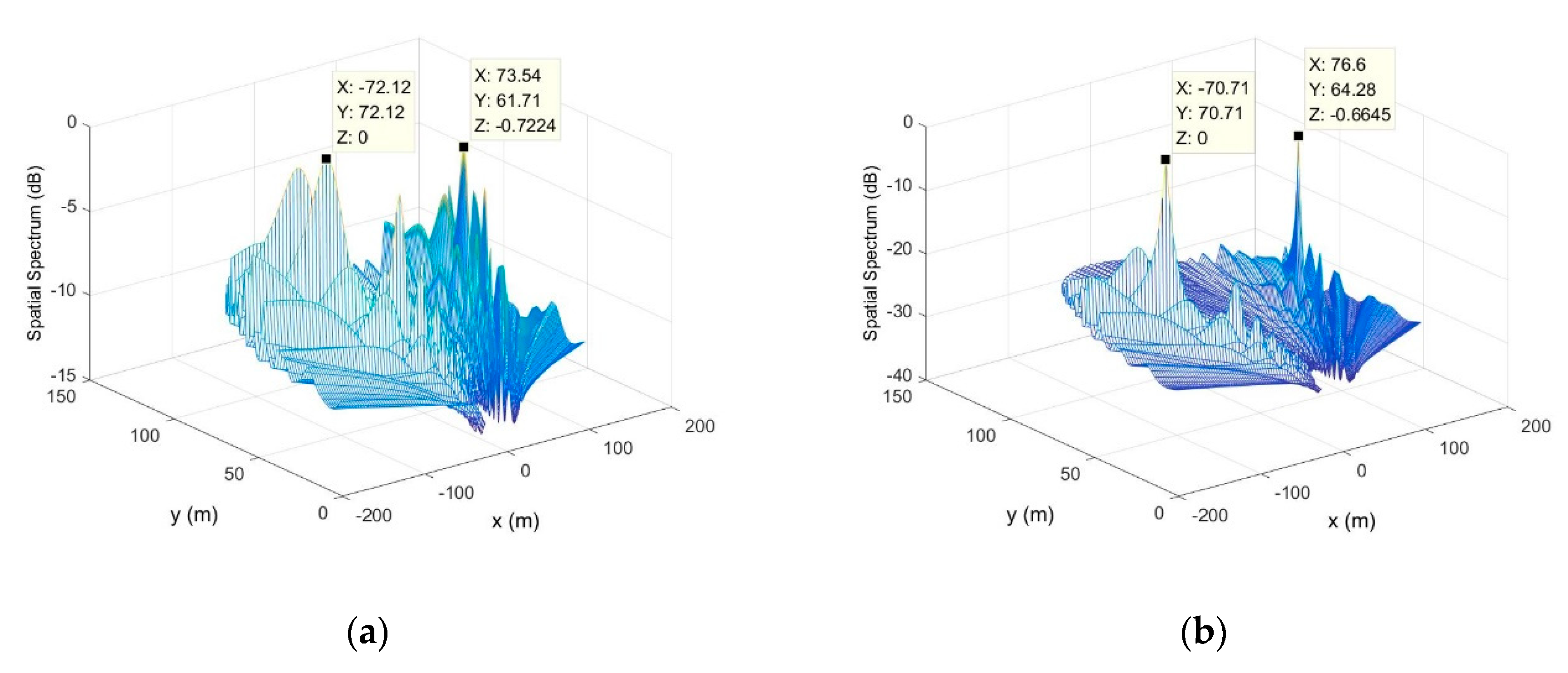
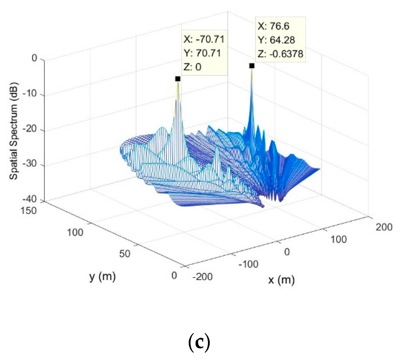
4.1.3. Multipath Compensation Strategy for Auxiliary Calibration (MLM-GC)

The water depth is 25 m. The multi-path model only includes the direct sound, the sea surface, and the sea bottom once reflected sound. The sea surface and bottom reflection coefficients are −0.9 and 0.3 respectively. Other condition is the same with Section 3.1. Figure 10 shows the simulation results of EV-GC, ML-GC, EVM-GC, and MLM-GC. EVM-GC is shown in reference [12], and it is an improved EV-GC for multipath environment. By comparison, it can be seen that the results obtained by ML-GC are less affected by the multipath method than the results obtained by EV-GC. The error of EV-GC is about 1.04 d, and the error of ML-GC is about 0.22 d. EVM-GC and MLM-GC can achieve a good estimation in multipath environment. The error of EVM-GC is about 0.02 d, and the error of MLM-GC is about 0.01 d.

The following part quantitatively analyzes the influence of the reflection coefficient estimation accuracy on the MLM-GC and EVM-GC. The ocean channel can be regarded as a slowly time varying and coherent multipath channel, but because of the sea surface fluctuations, platform sways, etc., the estimated multipath reflection coefficient often has some errors. The simulation conditions remain unchanged. The estimation error of reflection coefficient obeys the Gaussian distribution with zero mean value.

Figure 11 shows the RMSE of the elements position estimation changing with the reflection coefficient estimation standard deviation.

It can be seen that in the strong multipath environment, EVM-GC and MLM-GC estimated errors increase with the increase of the reflection coefficient error, but still have some tolerance to it. MLM-GC has a higher estimation accuracy than EVM-GC with coefficient error. When reflection coefficient estimation standard deviation is 0.2, X-RMSE and Y-RMSE of EVM-GC are 0.084 d and 0.077 d, X-RMSE and Y-RMSE of MLM-GC are 0.052 d and 0.019 d.

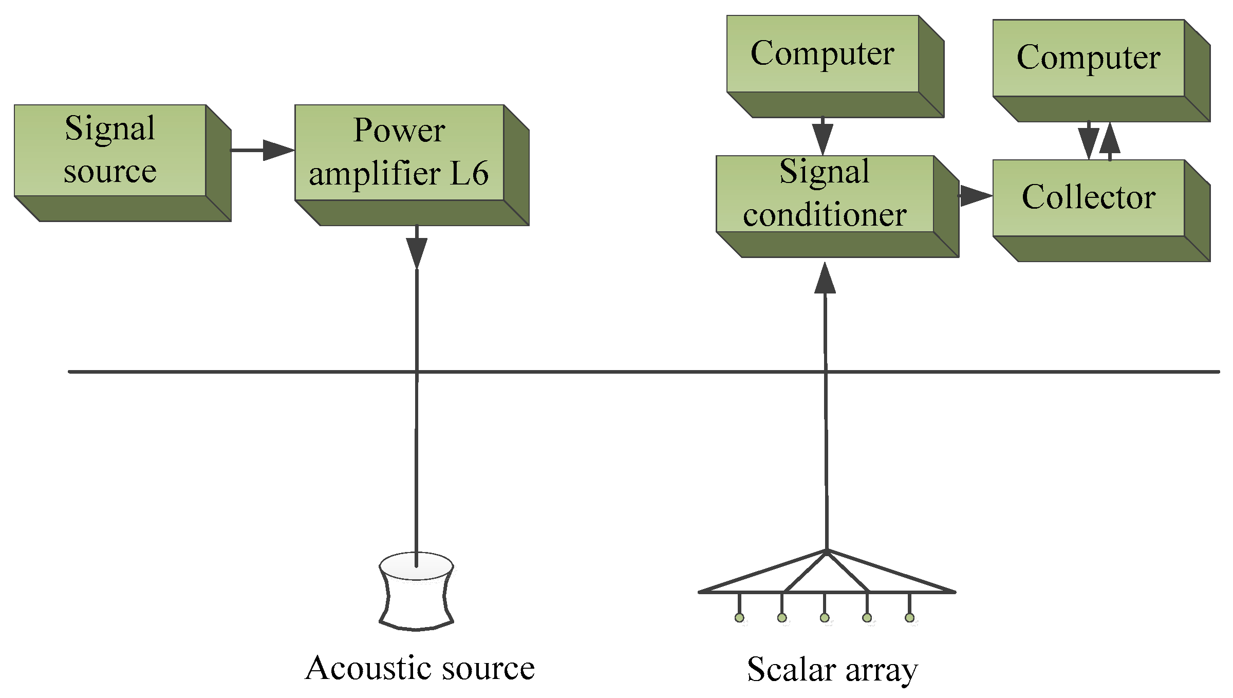
4.2. Lake Experiment

We performed a calibration experiment in Qiandao Lake. Figure 12 shows the experimental layout. The hydrophone array is a 5-element hydrophone linear array with a spacing of 0.2 m. The depth of the array element and the source is 2 m. The center of the array is the coordinate origin and the central array element is the reference array element. The source is 2.9 m away from the origin, and it meets the near-field condition. We just use one source, and change the DOA by rotating the array. The data measured in different DOAs are regarded as different source data. We use a broadband continuous noise signal, and the frequency is 1–6 kHz. The sampling rate is 51.2 kHz, and the sound velocity is 1458 m/s.

The DOAs of sources are −42.2° and −19.3°. We use the mean value of the calibration results of each narrowband signal (a sub-bandwidth is 100 Hz) as the final result. The calibration result is shown in Figure 13. Since the array elements are rigidly connected, the relative positional error among the array elements is small, and it is on the order of millimeters. However, the zeros degree reference in the experiment is measured with a tape measure, and there is a little azimuth deviation, so the calibration result in Figure 13 is considered to be reliable. Because the normalized sea surface reflection intensity is weak in the experiment, the multi-channel effect is not obvious. However, it can be seen from Figure 13 that the estimation result of MLM-GC is more approximate to a straight line than that of ML-GC.

Based on the above results, we analyze the near-field positioning accuracy before and after calibration. We set the target at −12°and 2.9 m. The near field focus positioning results are shown in

Table 4. Near-field target positioning results.

	DOA(Degree)		Distance(m)
	Estimated Value	Absolute Deviation	Estimated Value	Absolute Deviation
Before calibration	−14.9980	2.9980	2.8004	0.0996
ML−GC	−12.0000	0.0000	3.1999	0.2999
MLM−GC	−11.9976	0.0024	2.9004	0.0004

. It can be seen that, before calibration we use normal elements positions to locate the source, and the absolute deviation is 2.998°and 0.0996 m. ML-GC can improve the ability of DOA estimation, but the distance error becomes larger. MLM-GC achieves the best estimation here.

Next, the ML-GAC is verified. Here we use four sources that are not related both in time and space. The Formulas (17), (18), and (21) become,

$$F(\mathit{\alpha })={\displaystyle \sum _i\det \left[{\mathbf{P}}_A{}_i{\widehat{\mathbf{R}}}_i{\mathbf{P}}_A{}_i+\frac{\mathrm{tr}({\mathbf{P}}_A^{\perp }{}_i{\widehat{\mathbf{R}}}_i){\mathbf{P}}_A^{\perp }{}_i}{N-M}\right]},N\ne M,$$

(33)

where ${\widehat{\mathbf{R}}}_i$, ${\mathbf{P}}_A{}_i$, and ${\mathbf{P}}_A^{\perp }{}_i$ respectively express the covariance matrix of the $i$th received signal, the projection matrix of guide vector and the orthogonal component of ${\mathbf{P}}_A{}_i$, where they satisfy the following formula:

$${\mathbf{P}}_A{}_i=A_i{(A_i{}^{\mathrm{H}}{A}_i)}^{-1}{A}_i{}^{\mathrm{H}},$$

(34)

$${\mathbf{P}}_{Ai}^{\perp }=\mathbf{I}-{\mathbf{P}}_{Ai}.$$

(35)

The DOAs of the four sources are −40.2°, −19.3°, 3.9°, and 33.9°, and the distance are all 2.9 m. Other conditions are the same as above. Figure 14 and

Table 5. Estimation result of source position using ML-GAC.

Source Num.	1	2	3	4
Estimated DOA (°)	−37.7077	−18.6544	2.0127	31.4406
DOA Deviation (°)	2.4923	0.6456	1.8873	2.4594
Estimated Distance (m)	2.9546	2.5808	3.0798	2.9311
Distance Deviation (m)	0.0546	0.3192	0.1798	0.0311

are the joint estimation results of the elements and source positions using ML-GAC.

The above experiment proves the validity of ML-GAC. Because this method does not require the known source position, and the baseline is determined by the ordinate of the central array element and the 4th element, so the position estimation result of the elements is not affected by the 0° deviation. However, the accuracy of the source joint positioning is significantly lower than that of the auxiliary correction method. It should be noted that the 0° reference error is included in the DOA deviation in Table 5, which is caused by inaccurate preset azimuth.

5. Conclusions

This paper proposes a near-field element position calibration method which can be used for auxiliary calibration and self-calibration. The method is based on the near-field element position error model. Using the non-conditional maximum likelihood estimator, we construct an objective function, and the DE method are used to solve the problem of near-field calibration. Considering the underwater multipath influence, this paper compensates the mapping model according to linear acoustic theory and feature decomposition properties. Then we obtain a robust high-precision near-field element position matching calibration method that can be used in strong multipath environments. The main conclusions of this paper include: (1) the proposed calibration method based on maximum likelihood estimation can correctly estimate the position of array elements in strong multipath environment with source in near-field, and significantly improve the array positioning accuracy. The algorithm has certain tolerance for multipath reflection coefficient estimation error. (2) The position estimation of the array element RMSE is affected by the SNR, the number of snapshots, and the azimuth angle of the auxiliary sources. When the azimuth angles of different auxiliary sources are greater than 20°, the position estimation result of the array elements is more accurate. (3) The proposed method outperforms the eigenvector method especially under high SNR and multipath conditions, and the estimation accuracy can approach CRLB.

References

1. Yang, S.; Kainam, T.W.; Fangjiong, C. “Quasi-Blind” Calibration of an Array of Acoustic Vector-Sensors That Are Subject to GainErrors/Mis-Location/Mis-Orientation. IEEE Trans. Signal Process. 2014, 62, 2330–2344. [Google Scholar]
2. Ping, K.T.; Kainam, T.W.; Yang, S. An Hybrid Cramer-Rao Bound in Closed Form for Direction-of-Arrival Estimation by an “Acoustic Vector Sensor” With Gain-Phase Uncertainties. IEEE Trans. Signal Process. 2014, 62, 2504–2516. [Google Scholar]
3. Ye, T.; Yanru, W.; Xiaoliu, R. Mixed source localization and gain-phase perturbation calibration in partly calibrated symmetric uniform linear arrays. Signal Process. 2020, 166, 107267. [Google Scholar]
4. Schmidt, R.O. Multilinear array manifold interpolation. IEEE Trans. Signal Process. 1992, 40, 857–866. [Google Scholar] [CrossRef]
5. Boon, P.N.; Meng, H.E. A Gaid/Phase Calibration Technique for Adaptive Beamforming. In Proceedings of the ICCS, Singapore, 14–18 November 1994; Volume 3. [Google Scholar]
6. Lev, M.; Messer, H. Sufficient condition for array calibration using source of mixed tapes. In Proceedings of the ICASSP, Albuquerque, NM, USA, 3–6 April 1990; Volume 5, pp. 2943–2946. [Google Scholar]
7. Weiss, A.J.; Friedlander, B. Array Shape Calibration Using Sources in Unknown Locations-A Maximum Likelihood Approach. IEEE Trans. Acoust. Speech Signal Process. 1989, 37, 1958–1966. [Google Scholar] [CrossRef]
8. Ng, B.P.; Lie, J.P.; Er, M.H.; Feng, A. A practical simple geometry and gain/phase calibration technique for antenna array processing. IEEE Trans. Antennas Propag. 2009, 57, 1963–1971. [Google Scholar]
9. Kim, H.; Haimovich, A.M.; Eldar, Y.C. Non-coherent direction of arrival estimation from magnitude-only measurements. IEEE Signal Process. Lett. 2015, 22, 925–929. [Google Scholar] [CrossRef]
10. Wang, Y.; Zou, N.; Liang, G. Auxiliary calibration method for near-field position of hydrophone array in strong multipath environment. Acta Phys. Sin. 2015, 64, 024304. [Google Scholar]
11. Minqiu, C.; Xi, C.; Xingpeng, M. A subspace-based Manifold separation technique for array calibration. In Proceedings of the ISSPIT, St. Raphael Resort, Limassol, Cyprus, 12–14 December 2016; pp. 40–44. [Google Scholar]
12. Nan, Z.; Yan, W.; Jin, F.; Guolong, L. A Geometry Calibration Technique for Hydrophone Array with Sources in Near Field. J. Comput. Acoust. 2016, 23, 1540008. [Google Scholar]
13. Chen, Z.; Zhang, L.; Zhao, C.; Li, J. Calibration and Evaluation of a Circular Antenna Array for HF Radar Based on AIS Information. IEEE Geosci. Remote Sens. Lett. 2020, 17, 988–992. [Google Scholar] [CrossRef]
14. Wang, D.; Wu, Y. A Novel Array Errors Auxiliary calibration Algorithm. Acta Electron. Sin. 2010, 38, 517–527. [Google Scholar] [CrossRef]
15. Wu, Y.; Leshem, A.; Wijnholds, S.J. A computationally efficient calibration algorithm for the LOFAR radio astronomical array. In Proceedings of the ICASSP, Florence, Italy, 4–9 May 2014; pp. 5402–5406. [Google Scholar]
16. Weiss, A.J.; Friedlander, B. Array shape calibration using eigenstructure methods. Signal Process. 1991, 22, 251–258. [Google Scholar] [CrossRef]
17. Eric, K.L.; Hung, A. Critical Study of a Self-calibrating Direction-Finding Method for Arrays. IEEE Trans. Signal Process. 1994, 42, 471–474. [Google Scholar]
18. Kim, K.S.; Yang, E.; Myung, N.H. Self-calibration of an active uniform linear array using phase gradient characteristics. IEEE Antennas Wirel. Propag. Lett. 2019, 18, 497–501. [Google Scholar] [CrossRef]
19. Jiajia, Z.; Hui, C.; Weiping, H.; Weijian, L. Self-Calibration of Mutual Coupling for Non-uniform Cross-Array. Circuits Syst. Signal Process. 2019, 38, 1137–1156. [Google Scholar]
20. Ng, B.P.; Er, M.H.; Kot, C. Array gainlphase calibration techniques for adaptive beamforming and direction finding. IEEE Proc. Radar Sonar Navig. 1994, 141, 25–29. [Google Scholar] [CrossRef]
21. Dajun, S.; Xiaoping, H.; Hongyu, C. Iterative multi-channel FH-MFSK reception in mobile shallow underwater acoustic channels. IET Commun. 2020, 14, 838–945. [Google Scholar]
22. Van Trees, H.L. Optimum Array Processing; Wiley-Interscience: New York, NY, USA, 2002; pp. 746–762. [Google Scholar]
23. Wan, S.; Chung, P.J.; Mulgrew, B. Maximum likelihood array calibration using particleswarm optimisation. IET Signal Process. 2012, 6, 456–465. [Google Scholar] [CrossRef]
24. Tahere, Y. Parameter optimization of software reliability models using improved differential evolution algorithm. Math. Comput. Simul. 2020, 177, 46–62. [Google Scholar]
25. Jaroslaw, B.; Bartosz, K.; Alina, M. Local Levenberg-Marquardt Algorithm for Learning Feedforward Neural Networks. J. Artif. Intell. Soft Comput. Res. 2020, 10, 299–316. [Google Scholar]
26. Gang, Q.; Qingjun, S.; Lu, M. Channel prediction based temporal multiple sparse bayesian learning for channel estimation in fast time-varying underwater acoustic OFDM communications. Signal Process. 2020, 175, 107668. [Google Scholar]
Figure 1. Near-field spherical wave model with geometry error, the i th source s i , range between source and element r , direction of arrival φ i , the n th element actual position ρ n = ( x n , y n ) , the n th element normal position ( x 0 n , y 0 n ) .
Jmse 08 00678 g001
Figure 2. Results of ML-GC.
Jmse 08 00678 g002
Figure 3. Spatial spectrums before and after calibration. (a) Spatial spectrum without calibration; (b) spatial spectrum with actual elements positions; (c) spatial spectrum with ML-GC estimated positions.
Jmse 08 00678 g003aJmse 08 00678 g003b
Figure 4. RMSE of array shape estimation with signal-to-noise ratio (SNR) increasing under different numbers of snapshots. (a) EV-GC; (b) ML-GC.
Jmse 08 00678 g004
Figure 5. Comparison of estimation errors with and without source errors. (a) EV-GC; (b) ML-GC.
Jmse 08 00678 g005
Figure 6. RMSE of array shape estimation with different DOAs of auxiliary sources. (a) EV-GC; (b) ML-GC.
Jmse 08 00678 g006
Figure 7. Calibration result of ML-GAC.
Jmse 08 00678 g007
Figure 8. RMSE of ML-GAC with SNR increasing under different numbers of snaps. (a) Array position estimation; (b) source location estimation.
Jmse 08 00678 g008
Figure 9. The RMSE of the elements and the sources position estimation changing with the target azimuth based on ML-GAC. (a) Estimation RMSE of elements position in X direction; (b) estimation RMSE of elements position in Y direction; (c) estimation RMSE of target distance; (d) estimation RMSE of target direction of arrival (DOA).
Jmse 08 00678 g009
Figure 10. Calibration result of elements position with strong multipath. (a) EV-GC; (b) ML-GC; (c) EVM-GC; (d) MLM-GC.
Jmse 08 00678 g010aJmse 08 00678 g010b
Figure 11. RMSE of array shape estimation with different coefficient error of strong multipath. (a) EVM-GC; (b) MLM-GC.
Jmse 08 00678 g011
Figure 12. Experiment layout.
Jmse 08 00678 g012
Figure 13. Array position calibration result.
Jmse 08 00678 g013
Figure 14. Array position calibration result using ML-GAC.
Jmse 08 00678 g014