Investigation of the Flow Field of a Ship in Planar Motion Mechanism Tests by the Vortex Identification Method

Abstract

Planar motion mechanism (PMM) tests provide a means of obtaining the hydrodynamic derivatives needed to assess ship maneuverability properties. In this paper, the self-developed computational fluid dynamic (CFD) solver based on the open source code platform OpenFOAM, naoe-FOAM-SJTU, associated with the overset grid method is used to simulate the complex viscous flow field of PMM tests for a benchmark model Yupeng Ship. This paper discusses the effect of several parameters such as the drift angle and period on the hydrodynamic performance of the ship and compares the time histories of the predicted forces and moments with experimental data. To investigate the complex viscous flows with a large separation, four vortex identification methods are used to capture the vortex structures. The results show that the forces and moments are in good agreement in static drift and dynamic tests. By comparing the vortex structures, it is found that the third generation vortex identification methods, OmegaR and Liutex, are able to more accurately capture the vortex structures. The paper concludes that the present numerical scheme is reliable and the third generation vortex identification methods are more suitable for displaying the vortex structures in a complex viscous flow field.

1. Introduction

The accurate assessment of ship maneuverability in the design stage is essential for the safe navigation and efficient operation of ships. The International Maritime Organization adopted the “Standards for Ship Maneuverability” in 1993, which provided provisions and recommendations for ship maneuverability indicators. The accuracy of ship maneuverability prediction relies on the quality of the hydrodynamic derivatives estimation. The planar motion mechanism (PMM) test is a widely applied method to obtain the hydrodynamic derivatives of a ship, including the static drift, pure sway and pure yaw tests. Nowadays, the ship maneuvering behavior is mainly predicted by direct, experimental and numerical methods. As a powerful and efficient tool, the popularity of computational fluid dynamics (CFD) is increasing rapidly in the prediction of ship maneuverability.

Tahara et al. [1] used self-developed solver to predict the hydrodynamic characteristics of S60 at different drift angles. In their study, the mesh independency was carried out by five grids resolutions. Simonsen and Stern [2] simulated the oblique towing test of Esso Osaka. However, the free surface was ignored in the numerical simulations. Pinto-Heredero et al. [3] adopted the solver, CFD Ship-Iowa, to simulate the flow field of the Wigley ship with the drift angle from 10° to 60°. The free surface was captured by the level-set method. Ismail et al. [4] conducted the numerical simulations of the KVLCC2 model with the drift angle from 0° and 12°. They found that a second-order total variation diminishing (TVD) scheme was more suitable to predict the forces/moments acting on the hull. Xing et al. [5] also used the solver, CFD Ship-Iowa, to carry out numerical simulations of oblique towing tests of a KVLCC2 tanker at different drift angles (0°, 12°, 30°). In the study, a detached eddy simulation (DES) was applied to capture the flow separation phenomenon and the vortex structures around the hull. In the numerical simulations, the total number of grids was 13.0 million. However, the free surface was not taken into account. Stern et al. [6] summarized the numerical schemes in the simulation of ship maneuverability and found that using the DES method combined with enough grid refinement can obtain a more accurate numerical prediction. Meng and Wan [7] used the unsteady Reynolds averaged Navier–Stokes (RANS) to simulate the flow field of KVLCC2M at different drift angles in deep and shallow water. The connected vessels’ effect in shallow water was captured and abundant information in the flow field was presented. Wang et al. [8] simulated the flow field of ship hull at six drift angles by the CFD solver, naoe-FOAM-SJTU. The predicted hydrodynamic derivatives were in good agreement with the experiments.

Broglia et al. [9] conducted numerical predictions for the dynamic pure sway and pure sway tests of KVLCC1 and KVLCC2. They found that the stern of hull was the main region inducing the lateral force. Toxopeus et al. [10] adopted the dynamic mesh to realize the ship motion of KVLCC2 with full appendages. The predicted lateral force and yawing moment were in good agreement with the experiments. Cura-Hochbaum et al. [11] also carried out the numerical simulation of the dynamic test of KVLCC1 tanker based on RANS equations. The predicted hydrodynamic derivatives agreed well with the experiment results. Simonsen and Stern [12] simulated the pure yaw test of KRISO Container Ship (KCS) and analyzed the uncertainty of forces/moments acting on the hull. Sakamoto et al. [13,14] and Yoon et al. [15,16] used the solver, CFD Ship-Iowa, to simulate the static and dynamic PMM tests of DTMB 5415. The predicted hydrodynamic derivatives were compared with the test results, and the highest number of errors of linear hydrodynamic derivatives was less than 10%. Kim et al. [17] simulated the PMM test for a KCS ship by the CFD solver SHIP Motion. The predicted results of the static drift test and the dynamic pure sway test were in good agreement with the tests, but the predicted results of the pure yaw test were not accurate enough. Yang et al. [18] simulated the pure sway tests of the hull in deep and shallow water by solving unsteady RANS equations. However, the free surface was not taken into consideration in the numerical simulations. The effect of speed and water depth on the hydrodynamic performance of the hull in the pure sway test was investigated by Liu et al. [19]. In their studies, the CFD solver, naoe-FOAM-SJTU, was used to solve unsteady RANS equations by coupling it with the shear stress transport (SST) k-ω turbulence model. The lateral force and yawing moment increased rapidly. Wang and Wan [20] also adopted the CFD solver, naoe-FOAM-SJTU, to simulate the dynamic tests of DTMB 5415, and the solver was coupled with the overset grid technology. The predicted hydrodynamic derivatives were in good agreement with the experiments.

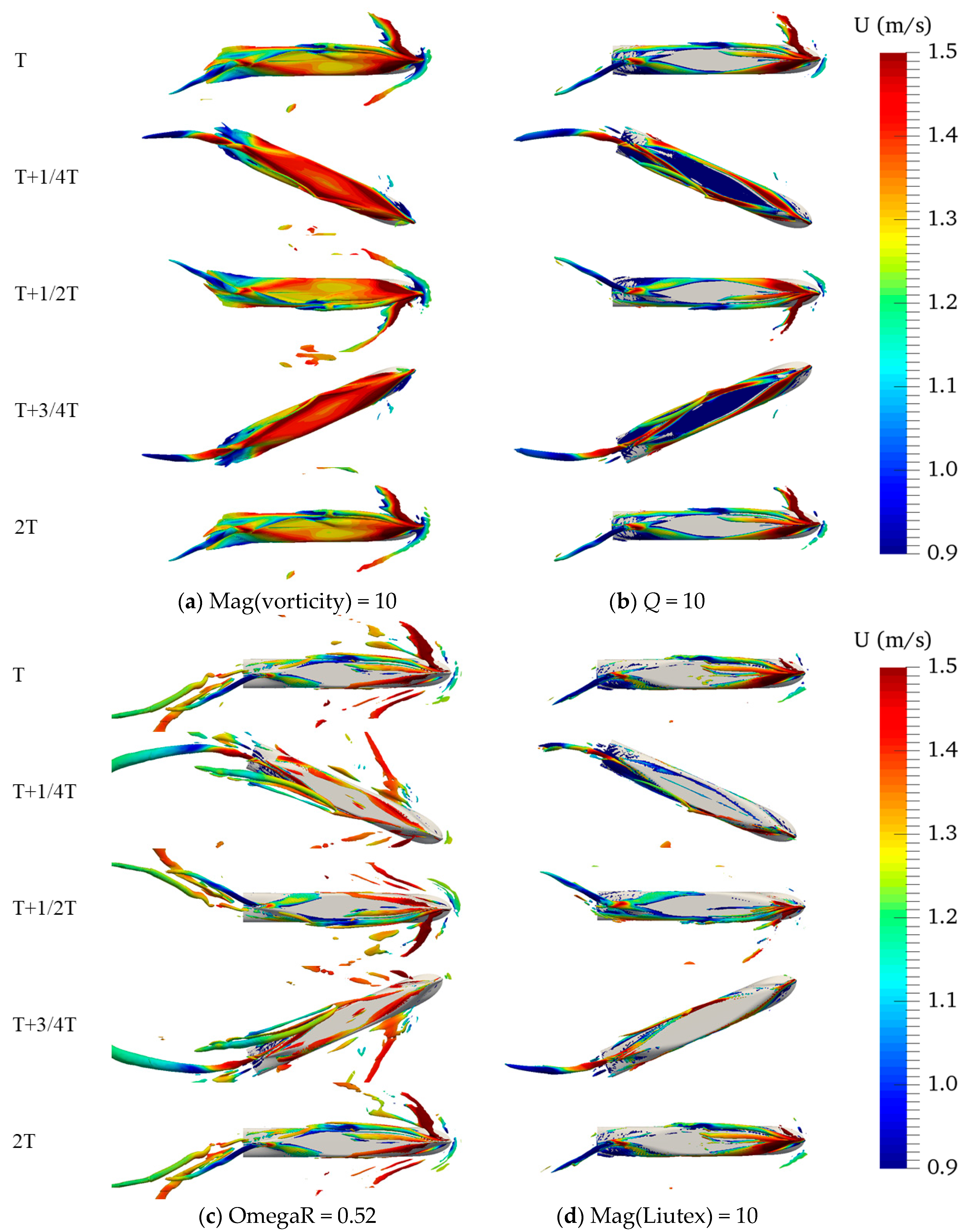
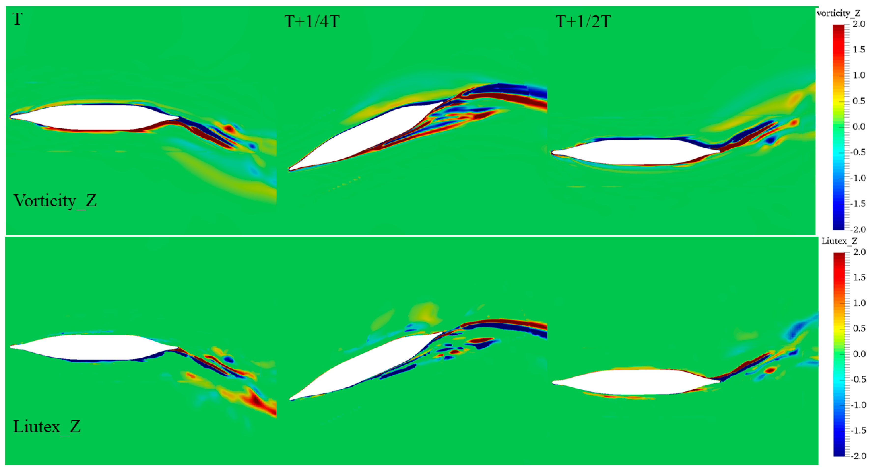
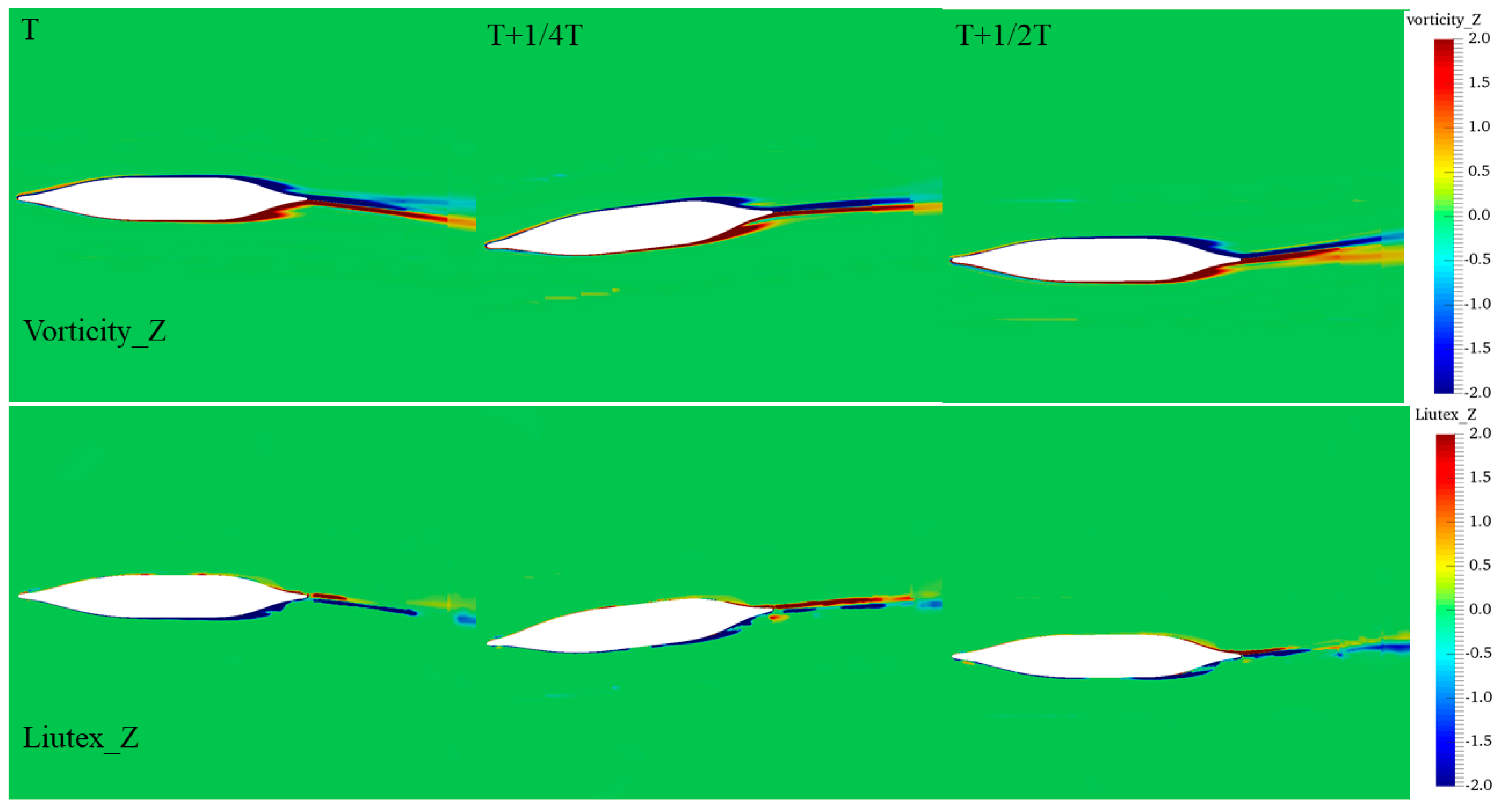
So far, the main aim of a ship planar motion mechanism is the hydrodynamic derivatives of the hull. There are few studies to simulate the detailed flow field in the larger separation flow, especially by using the new vortex identification methods. In this paper, reliable numerical schemes are presented, and four vortex identification methods are applied to analyze the separation flow in the PMM tests of a Yupeng ship.

In the present work, the authors perform the numerical simulations of static drift tests and dynamic tests of a Yupeng Ship. The CFD solver, naoe-FOAM-SJTU, is applied in the numerical simulations. Unsteady RANS equations coupled with an SST k-ω turbulence model are adopted to solve the flow field. The main framework of this paper goes as follows. The first part is the basic numerical methods and the vortex identification methods. The second part is the geometry model, grid generation and test conditions. Then comes the results and analysis, which contains the predicted results of the static drift, pure sway and pure yaw tests of the Yupeng Ship. In this section, the forces/moment, free surface, dynamic pressure and vortex structures are presented. Finally, the conclusion of this paper is drawn.

2. Numerical Methods

2.1. Basic Numerical Scheme

In this paper, the self-developed CFD solver, naoe-FOAM-SJTU, is used to perform the numerical simulations of the PMM tests. In the numerical computations, the governing equations are the unsteady Reynolds averaged Navier–Stokes equations, which are as follows:

$$\nabla ·\mathbf{U}=0$$

(1)

$$\frac{\partial \rho \mathbf{U}}{\partial t}+\nabla ·\left(\rho (\mathbf{U}-{\mathbf{U}}_{\mathbf{g}})\mathbf{U}\right)=-\nabla p_d-\mathbf{g}·\mathbf{x}\nabla \rho +\nabla ·({\mu }_{eff}\nabla \mathbf{U})+(\nabla \mathbf{U})·\nabla {\mu }_{eff}+f_{\sigma }$$

(2)

where U and U_g are the fluid velocity field and the grid velocity, respectively; p_d represents the dynamic pressure; μ_eff is the effective dynamic viscosity. f_σ is the surface tension term; ρ represents the density of the fluid and g is the gravity acceleration.

In the numerical calculations, the shear stress transport turbulence model, SST k-ω model, is selected to enclosure the URANS equations. The SST k-ω model is one of the widely used turbulence models and the model combines the advantages of the standard k-ε model and k-ω model to improve the accuracy when solving the free surface and near-wall region. In addition, it is noted that the rotation/curvature correction [21] of the SST k-ω model is added into the governing equations for capturing the vortex structures better. The free surface is captured by the volume of fluid (VOF) approach. The relative proportion of different fluids in the grid cell is expressed as:

$$\{\begin{array}{ll}\alpha =0& air\\ \alpha =1& water\\ 0<\alpha <1& interface\end{array}$$

(3)

where α represents the relative proportion. When it equals 0, it means that the grid cell is completely filled with air. When it equals 1, the cell is filled with water fully.

In the present numerical/experimental setup, the amplitude of sway motion in the dynamic tests can be as large as the beam of the ship model. Therefore, it is necessary to apply the dynamic overset grid method in the present numerical simulations to avoid the numerical error caused by grid deformation and improving the predicted accuracy. The transformation between the different computational domains is achieved by the Suggar++ library [22].

The velocity and pressure equations are decoupled by the merged PIMPLE (PISO-SIMPLE) algorithm. The algorithm allows the iterative procedure and pressure–velocity correction to solve the Navier–Stokes equations. In addition, built-in numerical schemes in OpenFOAM are applied to solve the partial differential equations (PDEs). A second-order TVD limited linear scheme is used to discretize the convection terms and the diffusion terms are approximated by a second-order central difference scheme.

2.2. Vortex Identification Methods

2.2.1. First Generation of Vorticity-Based Vortex Identification Methods

The first generation of vortex identification methods is based on the definition of vorticity proposed by Helmholtz in 1858. The vorticity is defined as velocity curl, ∇×U. Based on the Cauchy–Stokes decomposition, it is considered to be twice the rotational angular velocity of the rigid body rotation angular velocity of the fluid mass. The Cauchy–Stokes decomposition [23] is expressed as:

$$U\left(r+dr\right)=U\left(r\right)+Adr+\frac{1}{2}\omega \times dr$$

(4)

According to the decomposition, U is the velocity vector and r is radius vector. The movement of fluid mass can be decomposed into three parts: translation, symmetrical tensor A and vorticity ω. In this method, the vorticity ω represents the rigid body rotating part of the fluid mass movement.

2.2.2. Second Generation of Eigenvalue-Based Vortex Identification Methods

The second generation encompasses modifications based on the first generation. Both methods are derived from the Cauchy–Stokes decomposition. The second generation of vortex identification methods includes Q, λ₂, Δ, and λ_ci. Here is a brief introduction of the Q criterion. The Q criterion is a widely used vortex identification methods. The expression [23] can be written as:

$$Q=\frac{1}{2}\left({\Vert B\Vert }_F^2-{\Vert A\Vert }_F^2\right)$$

(5)

where A and B represent the symmetric and antisymmetric parts of the velocity gradient tensor, respectively.

However, in this method, the threshold of Q had to be selected manually, so that the threshold has an important influence on the display of the vortex structure.

2.2.3. Third Generation of Vortex Identification Methods

Liu et al. [23] proposed the third vortex identification methods: OmegaR and Liutex/Rortex.

The OmegaR method was also derived from the Cauchy–Stokes decomposition. In this method, the vorticity ω is further decomposed into a rotating part and a nonrotating part. The Ω [23] can be expressed as:

$$\mathsf{\Omega }=\frac{{\Vert B\Vert }_F^2}{{\Vert A\Vert }_F^2+{\Vert B\Vert }_F^2+\epsilon }$$

(6)

Obviously, Ω is between 0 and 1, which can be understood as the concentration of vorticity. Ω = 0.51 or 0.52 are always selected as a fixed threshold to identify the vortex structure. ε is a small positive number for avoiding a division by zero. The OmegaR method avoids the problem of artificially adjusting the threshold.

According to the Cauchy–Stokes decomposition, the antisymmetric tensor B cannot represent the rigid body part of fluid motion. The Liutex/Rortex vector systematically solves the problem to obtain a rigid rotating part from the fluid motion. The Liutex vector [23] is defined as:

$$R=\left(\langle \omega ,r\rangle -\sqrt{{\langle \omega ,r\rangle }^2-4{\lambda }_{ci}^2}\right)r$$

(7)

where ω is the vorticity vector.

The Liutex vector represents not only the rotation intensity, but also the local rotation axis; compared with the Cauchy–Stokes decomposition, the Liutex vector provides an accurate motion decomposition to capture the rigid rotation part in the flow field.

3. Numerical Simulation Setup

3.1. Geometry Model

In the present study, the benchmark model, Yupeng Ship, is used for all the computations. The geometry model of Yupeng Ship is shown in Figure 1. The principle particulars are listed in

Table 1. Principle particulars of a Yupeng Ship.

Main Particulars	Symbols	Unit	Full Scale
Length between perpendiculars	Lpp	m	189
Beam	BWL	m	27.8
Draft	TM	m	10.3
Displacement volume	∇	m3	39,019
Initial stability	GM	m	1.18
Block coefficient	CB		0.721
Longitudinal inertial radius	Ryy	m	48.206
Speed		kn	18

. In the numerical simulations, a model scale is adopted and the scale ratio is 1:49. The length between the perpendiculars of the ship model is 3.857 m. The researchers of Marine Design and Research Institute of China (MARIC) conducted extensive experiments using the model ship. In the experiments, the speed of ship model is 1.323 m/s, corresponding to Fr = 0.215. In the PMM tests, the heave and pitch motion are taken into consideration.

3.2. Tests and Calculated Conditions

In the experiments, the static drift and dynamic tests were carried out in the towing tank of MARIC. The test conditions are summarized and listed in

Table 2. Summary of the tests and calculated conditions.

Conditions	CASE	Amplitude (m)	Period (s)	Drift Angle (°)
Static drift test	DA4	-	-	4
	DA20	-	-	20
Dynamic pure sway test	PS8	0.4	8	-
	PS16	0.4	16	-
Dynamic pure yaw test	PY8	0.4	8	-
	PY16	0.4	16	-

. The static drift tests included two conditions, namely drift angle 4° and 20°. The dynamic tests included the pure sway and pure yaw tests. In the dynamic tests, the amplitude of the sway motion is 0.4 m. The periods of pure sway motions are 8 s and 16 s, respectively. The periods of pure yaw motions are the same with pure sway tests. The calculation reference point of forces and moments is the center of gravity.

3.3. Grids Generation

In order to simulate the large amplitude motion of the Yupeng ship, the dynamic overset mesh is adopted in the present numerical calculations. The computational domain and boundary conditions are presented in Figure 2. The computational domain is −1.0 L_pp ≤ x ≤ 3.0 L_pp in length, −1.5 L_pp ≤ y ≤ 1.5 L_pp in width and −1.0 L_pp ≤ z ≤ 0.5 L_pp in height. The red line indicates the boundary of the overlap domain. In the present simulations, the grid is generated by the commercial software, Hexpress. The grids of the background and hull domain are generated respectively. To capture the free surface accurately, a block is adopted to refine the grid near the free surface. The total grid number is about 6.28 million. The grid distribution is shown in Figure 3. Figure 3a presents the global grid distribution. The red and blue lines depict the grid distribution of the background and hull domain, respectively. A box is used to refine the mesh around the hull. Figure 3b shows the grid distribution on the free surface. The grid distribution of the hull is depicted in Figure 3c.

To analyze the mesh independence, three mesh resolutions, with the refinement ratio of $\surd 2$, were adopted in the numerical simulations.

Table 3. Details of the mesh generation.

Grid Sets	Background Mesh (Million)	Hull Mesh (Million)	Total (Million)
Coarse	0.77	1.47	2.24
Mid	2.16	4.12	6.28
Fine	6.05	11.54	17.59

summaries the details of the mesh generated with different resolutions. As shown in the table, the mesh of the background and hull domain was refined. The grid number with fine resolution approaches 17.59 million. Figure 4 presents the grid distribution with different mesh resolutions at the longitudinal cutting plane.

The different grid distributions are adopted to simulate the hydrodynamic performance of the Yupeng Ship in CASE DA4. The predicted results are summarized in

Table 4. Grid convergence of the resistance in CASE DA4.

	Resistance (N)	Error	Lateral Force (N)	Error	Yawing Moment (NM)	Error
EFD	11.30	-	7.33	-	27.83	-
Coarse	9.89	−12.48%	7.45	1.64%	26.94	−3.20%
Mid	10.12	−10.44%	7.36	0.41%	27.28	−1.98%
Fine	10.23	−9.47%	7.34	0.14%	27.52	−1.11%

. Since the resistance is affected by many factors and fluctuates greatly in the experiments, the resistance was slightly over-predicted in the numerical simulations. However, the predicted lateral force and yawing moment are in good agreement with the experimental values, and all of their errors achieved by different mesh resolutions were less than 5%. The results of the fine mesh scheme were slightly improved compared to mid mesh scheme.

Taking the predicted accuracy and time-consumption into consideration, the mid mesh distribution is selected to carry out the next simulations.

4. Results and Discussion

In this section, all of the experimental conditions are simulated by the CFD solver, naoe-FOAM-SJTU. The predicted forces and moments are compared with the experiments. In the static drift tests, the values at the last 18 s of the prediction are plotted. The plotted values in the dynamic tests are the last two periods of the numerical simulations. All the numerical simulations are performed on the high performance computing (HPC) cluster center in Computational Marine Hydrodynamics Lab (CMHL), Shanghai Jiao Tong University. Each node consists of two Central Processing Units (CPUs) with 20 cores per node and 64GB accessible memory (Intel Xeon E5-2680v2 @2.8 GHz). In total, 40 processors are assigned for each case, in which 39 are for the calculation of the flow field and the other processor is for the interpolation calculation of the overset grids. In the numerical simulations, the time step is set to Δt = 0.0005 s, and the Courant number is less than 1.0 in the current predictions. Each calculation costs approximately 264 h with about 60,000 time steps.

4.1. Static Drift Test

4.1.1. Force and Moments

In the static drift tests, the forces and moments acting on the hull are greatly affected by the drift angle. The comparison between the experiments and the predicted results are presented in Figure 5. The left column is the results of the CASE DA4 tests and the right is the CASE DA20 tests. It can be seen that there are greater fluctuations in the experiment data and the predicted results are more regular. In CASE DA20, the forces and moments are greater than that in CASE DA4. The lateral force and yawing moment at drift angle 20° are much larger than the results at drift angle 4°. The errors between the experimental and predicted results are listed in

Table 5. Comparison between the predicted and experimental forces and moment in the static drift test.

CASE	Force/Moment	EFD	CFD	Error
DA4	Resistance (N)	11.30	10.32	−10.44%
	Lateral force (N)	7.33	7.36	0.43%
	Yawing moment (NM)	27.83	27.28	−1.98%
DA20	Resistance (N)	15.08	13.77	−8.69%
	Lateral force (N)	81.89	86.72	5.90%
	Yawing moment (NM)	127.80	125.28	−1.97%

. The forces and moment are the mean value of their time histories. There is the largest error in terms of the resistance in CASE DA4. The measured resistance, affected by many factors, leads to a great fluctuation of the time history, so that the predicted resistance is not very accurate. However, all the errors of the lateral force and yawing moment in both cases are less than 6%. The resistance and yawing moment are under-predicted compared to the experiments, while the lateral force is over-predicted. Overall, the predicted results are in good agreement with the experimental data.

4.1.2. Free Surface

The main advantage of CFDs over the experiment is that, not only can the hydrodynamic characteristics of the ship can be predicted, but a detailed flow field distribution around the hull can also be investigated. Figure 6 shows the comparison of the free surface at different drift angles. The static hydrodynamic characteristics of the hull can be explained to some extent by the wave-making pattern such as the height and length. As shown in Figure 6, the asymmetry of the wave-making wave pattern is more obvious at a larger drift angle. In addition, the range of the bow wave peak (starboard side) is wider and the peak value is larger. The dynamic pressure difference on both sides of the hull is intensified rapidly, caused by the increasing diffraction wave peak on the portside, so that the lateral force and yawing moment increase rapidly at the larger drift angle. In addition, the bow wave breaking is captured in CASE DA20, as shown in Figure 6c. The plunging wave breaking, which leads to the energy loss, is found in the evolution of diffraction waves on the portside.

4.1.3. Dynamic Pressure

Affected by the drift angle, the dynamic pressure distribution on the portside and starboard side is no longer symmetrical. The variation of the pressure distribution leads to the rapid change of the forces and moments. Figure 7 depicts the dynamic pressure distribution on the portside and starboard side of the Yupeng ship. Figure 7a shows the dynamic pressure on the portside. It is clear that the dynamic pressure in CASE DA20 is much lower than it is in other case. For the large drift angle case, the diffraction wave appears near the bow of the portside and the dynamic pressure decreases rapidly. Figure 7b shows the dynamic pressure distribution on the starboard side. The dynamic pressure near the bow of the starboard side at a larger drift angle is much larger than the results in CASE DA4. Compared with the dynamic pressure distribution on the portside, the difference of the dynamic pressure between both sides in CASE DA20 is much greater than the results of CASE DA4. Therefore, it results in a rapid increase in the lateral force and yawing moment.

4.1.4. Vortex Structure

Vortex structures around the hull, propeller and rudder are in different scales and intensities. In order to compare the behaviors of different vortex identification methods, the vortex structures obtained by four vortex identification methods are presented in Figure 8, where Figure 8a,b show the vortex structure in CASE DA4 and DA20, respectively. Overall, the hull is covered fully by the vortex structures based on vorticity in both cases. Obviously, the results are not acceptable. The Q criterion seems to more suitably capture the vortex structures in the flow field than the first generation method. As a third generation vortex identification method, the OmegaR method is able to capture larger and more vortex structures in the flow field. Compared to the results obtained by the OmegaR method, more broken vortex structures near the hull are captured by the Liutex method. Comparing the vortex structures in CASE DA4 and DA20, the vortex structure is longer and more complex at a larger drift angle. At larger drift angles (DA20), a vortex occurs on the portside of the hull. It is captured by the vortex identification method based on the vorticity, Q and the OmegaR method. It indicates that the large separation of field flow appears near the hull in CASE DA20 in the static drift tests.

In order to study the evolution of vortices along the ship longitudinal direction, a series of planes are selected to present the axial vorticity and Liutex. As shown in Figure 9, the vortex always appears in pairs with the alternate positive and negative value. The value of the axial vorticity is much larger than the value of axial Liutex. As shown in Figure 9a, there are ten pairs of vortices, eight of which are near the free surface, and the other two pairs occur near the bilge of the hull. By using the Liutex method, the vortex pairs are also captured clearly. Most of the vortex pairs also appear near the free surface, and there are two pairs of vortex near the bilge of the hull. The axial vorticity and Liutex occur at the same position, indicating that the strong rotating and separating motion appears near the bilge of the Yupeng Ship.

Figure 10 presents the evolution of vertical vorticity and Liutex at z/Lpp = −0.03572 along the ship length direction in CASE DA4 and DA20. At the small drift angle, the vertical vorticity and Liutex on the portside are very small and the flow separation is not very strong. The vertical vorticity and Liutex on the portside increase rapidly in CASE DA20. The violent flow separation appears on the portside at a large drift angle. Figure 10a presents the violent variation of the vertical vorticity in CASE DA20. The extensive vortices originates from the shoulder of the hull, while a pair of vertical Liutex originates from the mid-hull. Far from the hull, a vertical vorticity pair (V.P.) with an alternate positive and negative value is captured and the negative one is closer to the hull. By using the Liutex method, the vertical Liutex, which is similar to a Karman vortex street (K.V.S.), is displayed, as shown in Figure 10b.

4.2. Dynamic Test: Pure Sway

4.2.1. Force and Moments

In the dynamic tests, the forces and moments acting on the hull are smoother—especially the lateral forces and yawing moment. The predicted forces and moments in the pure sway tests are shown in Figure 11. It is obvious that the experimental resistance data fluctuate more sharply than the numerical results. Compared with the resistance in CASE PS8 and PS16, it is found that the pure sway period has little effect on ship resistance. The lateral force and yawing moment are affected significantly by the period of sway motion in the dynamic pure sway tests. The short period leads to a large lateral force and yawing moment. Although the forces and moments at different periods vary greatly, the lateral force and yawing moment in both cases are in good agreement with the experiment.

The errors between the experimental and predicted forces and moments are summarized in

Table 6. Comparison between the calculated and experimental forces and moment in pure sway tests.

CASE	Force/Moment	EFD	CFD	Error
PS8	Resistance (N)	12.65	11.96	−5.46%
	Lateral force (N)	165.61	158.03	−4.57%
	Yawing moment (NM)	109.88	99.66	−9.30%
PS16	Resistance (N)	11.54	10.11	−12.36%
	Lateral force (N)	45.81	40.50	−11.58%
	Yawing moment (NM)	49.74	45.75	−8.01%

. The resistance is the mean value at the last two periods. The lateral force and yawing moment are the amplitudes of the time histories and the amplitude is the mean of the four absolute peak values in the plots. As shown in the table, the resistance in CASE PS8 is slightly larger than that in CASE PS16, while the lateral force and yawing moment in the shorter period are much larger than the results of CASE PS16. Since the amplitude of the pure sway motion is the same, a smaller pure sway motion period leads to a higher sway acceleration, resulting in the larger lateral force and yawing moment. The predicted results of CASE PS18, whose errors are less than 10%, is relatively better than those of CASE PS16. Overall, the errors of forces and moment are less than 15%, which indicates that CFDs is able to accurately predict the forces and moments of the hull in the dynamic PMM tests.

4.2.2. Free Surface

Figure 12 shows the evolution of free surface wave-making in a period of pure sway test in CASE PS8. When the hull moves to the portside, the wave-making in the left flow field is squeezed and the amplitudes of wave-making near the bow and stern both increase, which corresponds to the lateral force pointing to the starboard side. Additionally, when the hull moves to starboard side, the trend of change is just the opposite way, which is due to the periodic lateral force and yawing moment, as shown in Figure 11.

4.2.3. Vortex Structure

The vortex structures in the dynamic pure sway test are obviously different from those in the static drift test. Figure 13 shows the vortex structure obtained by four methods in CASE PS8. The vortex structures obtained by four methods are all periodic. The vortex structures appearing on the bottom of the hull at one-quarter and three-quarter periods are also captured by these methods. It indicates that the separated flow occurs near the bottom of the hull. At T+1/4T, the vortex structures gradually approach the starboard side of the hull downstream. The trends of the vortex structures evolution at T+3/4T are opposite to one another. As shown in Figure 13a, the hull is covered fully by the vortex structures obtained based on the vorticity. Obviously, this is impossible in practice. The hull is covered partially by the vortex structures obtained by Q criterion. At T, the vortex structures mainly appear near the bilge of the hull. A vortex originates from the propeller shaft and tilts to the starboard side as it evolves downstream. At T+1/4T, a vortex occurs at the bottom of the hull, which starts from the mid-hull in the initial stage and gradually approaches the starboard side downstream. After separating from the hull at the bilge, it evolves downstream along the ship length direction. At T+1/2T, the pattern of the vortex structures is similar to the results at T, but the vortex that originated from the propeller shaft tilts to the portside downstream. Except for the vortex originated from the mid-hull, the distribution of vortex structures at T+3/4T are analogous to that at T+1/4T. The direction of the evolution of the vortex originated from the mid-hull is opposite to the results at T+1/4T. The vortex structures obtained by OmegaR are more complex and extensive vortices in the flow field are captured, especially near the free surface. However, the evolution of the main vortex is similar to the results obtained by the Q criterion. More broken vortices near the hull are captured by the Liutex method. At T, a vortex is captured at the bottom of the hull and evolves along the mid-hull, as shown in Figure 13d. The vortex is not visible in the results of the other methods.

Figure 14 and Figure 15 present the evolution of the vertical vorticity and Liutex at z/L_pp = −0.03572 along the ship length direction in CASE PS8 and PS16. Since the distribution in one period is basically symmetrical, the distribution in a half-period is only presented here. In CASE PS8, the flow separation is more obvious than that in CASE PS16, which is caused by a shorter period and it will lead to a larger sway velocity. The vertical vortex and Liutex presented in Figure 14 are larger than the results of CASE PS16. As shown in Figure 14, a larger vertical vorticity and Liutex are captured clearly near the stern of the hull, which indicates that a strong flow separation occurs. The violent flow separation causes a big loss of energy, resulting in the rapid increase in the lateral force and yawing moment. Compared with the vertical vorticity, the vertical Liutex is more disordered, and the value of the vertical Liutex is less than that of the vertical vorticity. Since the definition of vorticity and Liutex are different, the positive Liutex appears where a negative vorticity occurs.

4.3. Dynamic Test: Pure Yaw

4.3.1. Force and Moments

In the dynamic pure yaw tests, the predicted forces and moments are compared with the experiment, as shown in Figure 16. The left column shows the results of CASE PY8 and the right is the results of CASE PY16. Overall, the predicted forces and moment in both cases are in good agreement with the experiment. In CASE PY8, the resistance is also periodic, and there are two peaks in one period. In pure yaw tests, the resistance is also the largest when the drift angle of the hull reaches the maximum. It is more obvious in a shorter period. By comparing with the lateral force and yawing moment in CASE PY8 and PY16, it is found that a shorter period leads to a larger force and moment. The errors between the experimental and predicted forces and moment are listed in

Table 7. Comparison between the predicted and experimental forces and moment in pure yaw tests.

CASE	Force/Moment	EFD	CFD	Error
PY8	Resistance (N)	12.75	14.05	10.21%
	Lateral force (N)	77.78	91.53	17.67%
	Yawing moment (NM)	107.97	99.59	−7.76%
PY16	Resistance (N)	9.84	9.87	0.39%
	Lateral force (N)	16.28	17.48	7.33%
	Yawing moment (NM)	15.73	16.67	5.97%

. The resistance is calculated by the mean value of the time history at the last two periods and the lateral force and yawing moment are the average amplitudes of the time history. As shown in the table, the resistance in CASE PY8 is 40% larger than that in CASE PY16, and the lateral force and yawing moment are much larger than the results of CASE PY16. In both cases, the forces and moment predicted in the long period are more accurate than those in CASE PY8. The predicted results indicate that the numerical schemes adopted in the present study are reliable.

4.3.2. Free Surface

Figure 17 shows the evolution of the free surface wave-making in one period of CASE PY8. Compared with the results of CASE PS8, the variation of wave-making on the free surface around the hull is more drastic. Meanwhile, the peak of the bow wave is larger than that in the pure sway test due to the large yaw motion. In addition, there is a significant difference between the diffraction wave patterns on both sides of the hull. The bow wave breaking is also captured in CASE PY8. The periodic variation of wave-making leads to the corresponding change in the pressure field around the hull, resulting in the increment in the lateral force and yawing moment.

4.3.3. Vortex Structure

Since the yaw motion of the hull is taken into consideration, the vortex structures in the dynamic pure yaw test are obviously different from those in the pure sway tests. Figure 18 shows the vortex structures obtained by the different methods in CASE PY8. By observing the vortex structures obtained by the four methods, a vortex, which originated from the propeller shaft, is captured by all of them. The vortex structures near the bow are also visible to different extents. At T, the bow vortex structures near the free surface are captured by the method based on the vorticity, Q criterion and OmegaR, while more broken and fine vortex structures are presented by Liutex. At this time, the hull is moving to the portside, and the separation flow appears on the starboard side, which can be confirmed by the vortex structures near the bilge on the starboard. At T+1/4T, the bottom of the hull is covered by the vortex structures obtained by the Q criterion. Only the OmegaR method presents the bow vortex structures. Since the hull is swinging counterclockwise (see from bottom to top), the vortex structures originated from the mid-hull appear near the stern on the portside of the hull. The vortices are more clearly presented by Q, OmegaR and Liutex. At T+1/2T, the movement of the hull is the opposite to that at T, so the distribution of the vortex structures is basically symmetrical. The vortex structures originated from the propeller shaft approach the starboard side downstream. At T+3/4T, the hull swings clockwise, and the vortex structures occur at the mid-hull and approaches the starboard side downstream. At 2T, the distribution of vortex structures is basically the same as the results at T.

Figure 19 and Figure 20 present the evolution of the vertical vorticity and Liutex at z/L_pp = −0.03572 along the ship length direction in CASE PY8 and PY16. Similar to the phenomenon presented in the pure sway tests, the flow separation is more obvious in the shorter period. At T+1/4T, the drift angle in CASE PY8 is larger than that presented in Figure 20. Therefore, the flow separation on the portside is more violent in CASE PY8. At T and T+1/2T, the flow separates more obviously. This is because the lateral velocity becomes larger in a short period. It is confirmed by the vertical vorticity and Liutex near the stern of the hull. As shown in Figure 19, the Liutex method is able to capture more broken and finer vortices.

In summary, the characteristics of four vortex identification methods can be obtained by analyzing the capability of capturing the vortex structures in the ship’s large separation flow. As shown in

Table 8. Comparison of the different vortex identification methods.

Methods	Vortex Boundary	Threshold Sensitivity	Weak Vortex	Vortex Axis
Vorticity	No	sensitive	No	No
Q criterion	Yes	sensitive	No	No
OmegaR	Yes	insensitive	Yes	No
Liutex/Rortex	Yes	sensitive	No	Yes

, more information of vortex structures is displayed by the third generation of vortex identification methods, OmegaR and Liutex/Rortex.

5. Conclusions

In the present study, an in-house CFD solver, naoe-FOAM-SJTU, is used to perform numerical simulations of planar motion mechanism (PMM) tests of a Yupeng ship. Unsteady RANS equations combined with an SST k-ω turbulence model are adopted to solve the complex viscous flow and a dynamic overset grid method is applied to simulate the large amplitude motion of the hull. The paper not only compares the time histories of predicted and experimental forces and moments acting on the hull, but also uses four vortex identification methods to capture the vortex structures in the large separated flow, which are very helpful for a further analysis on the flow mechanism around the hull.

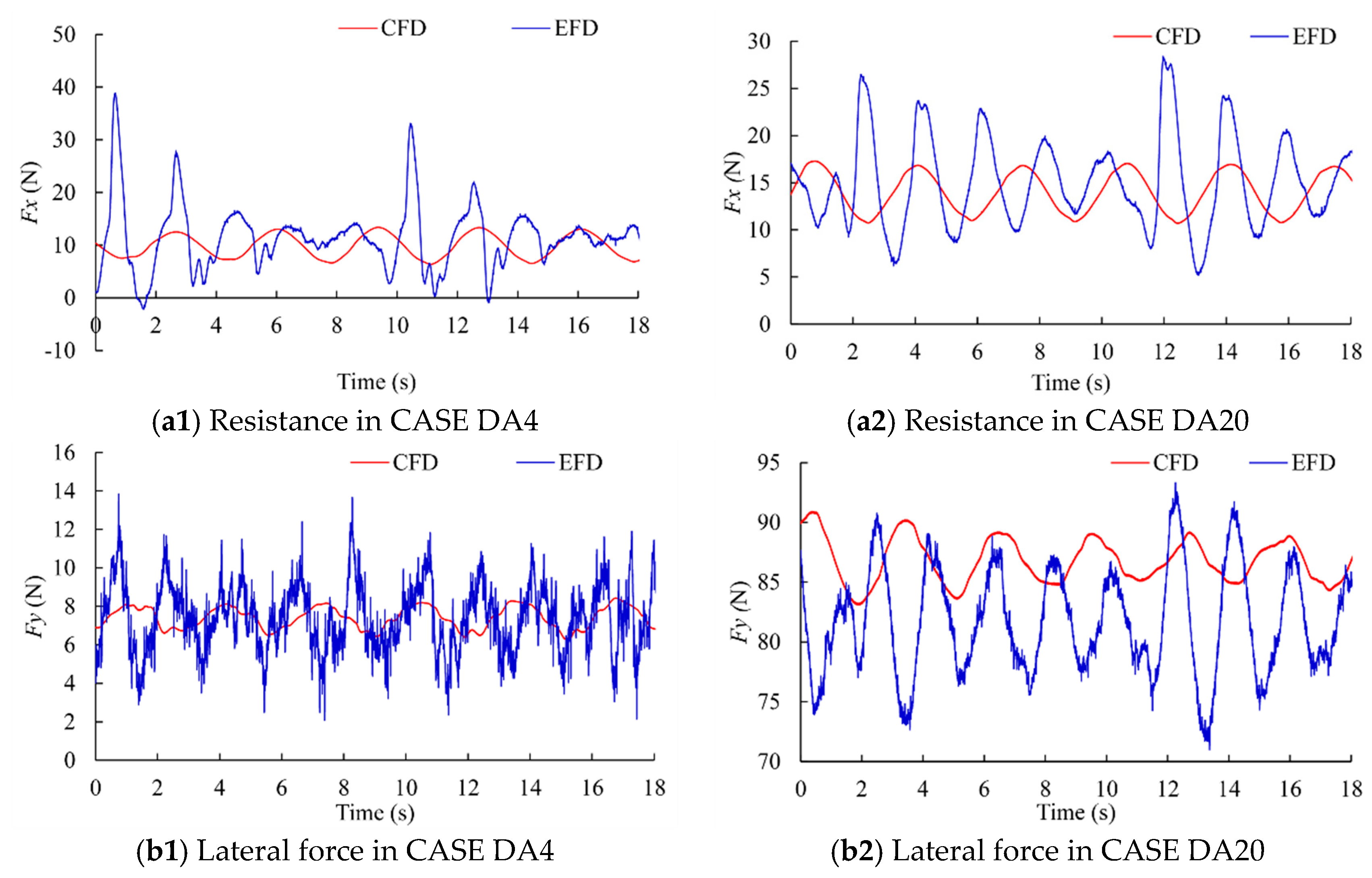
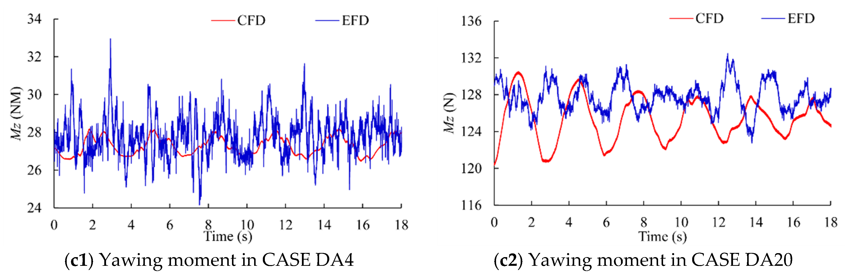
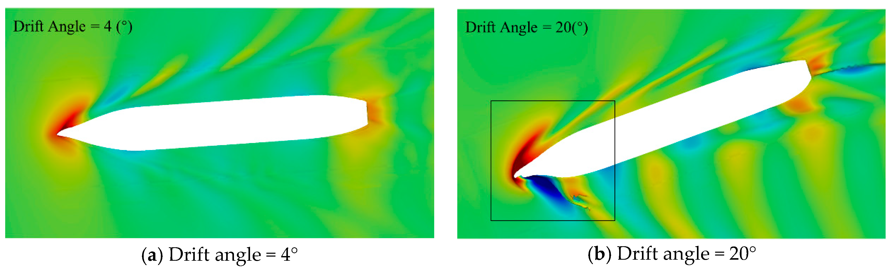
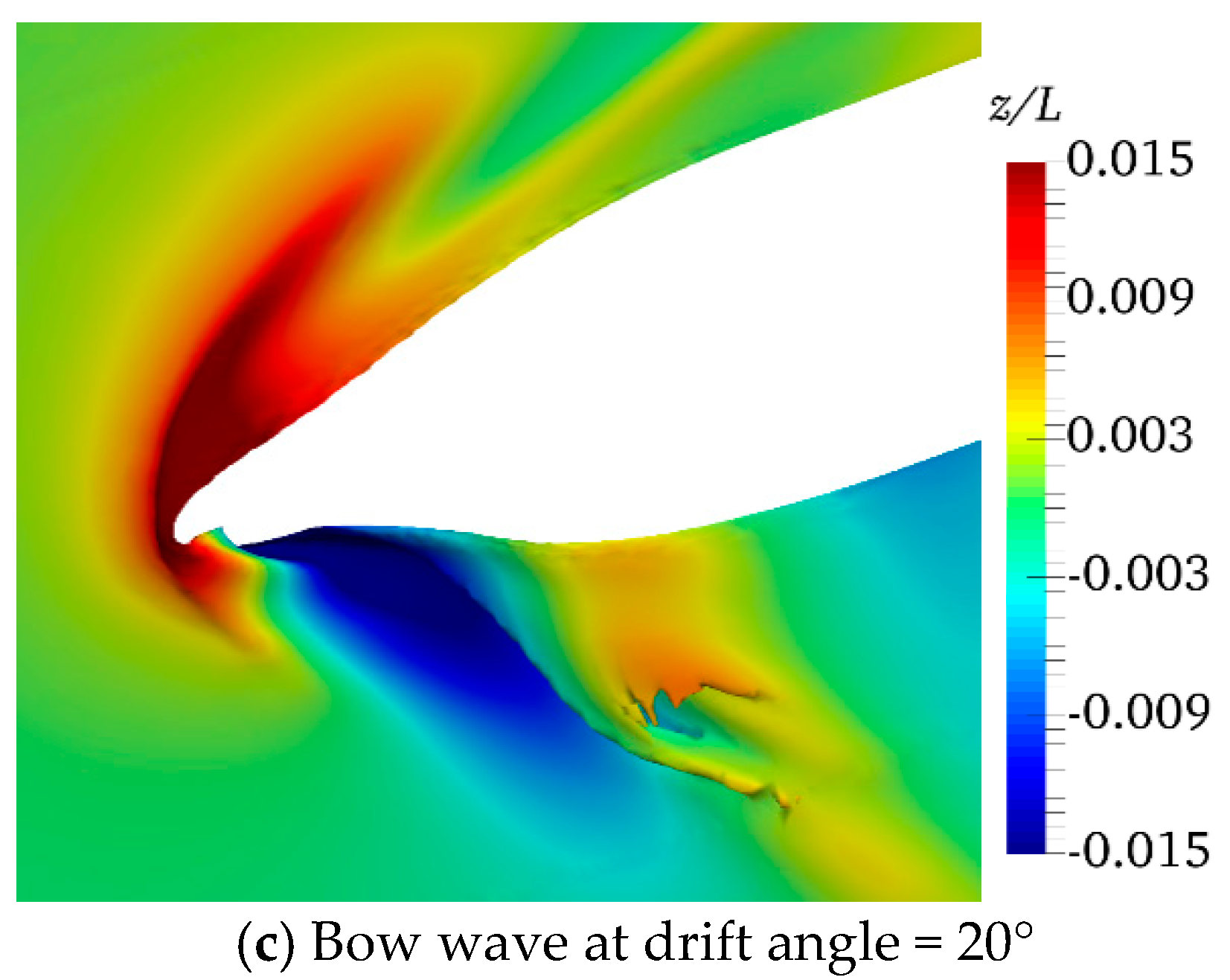
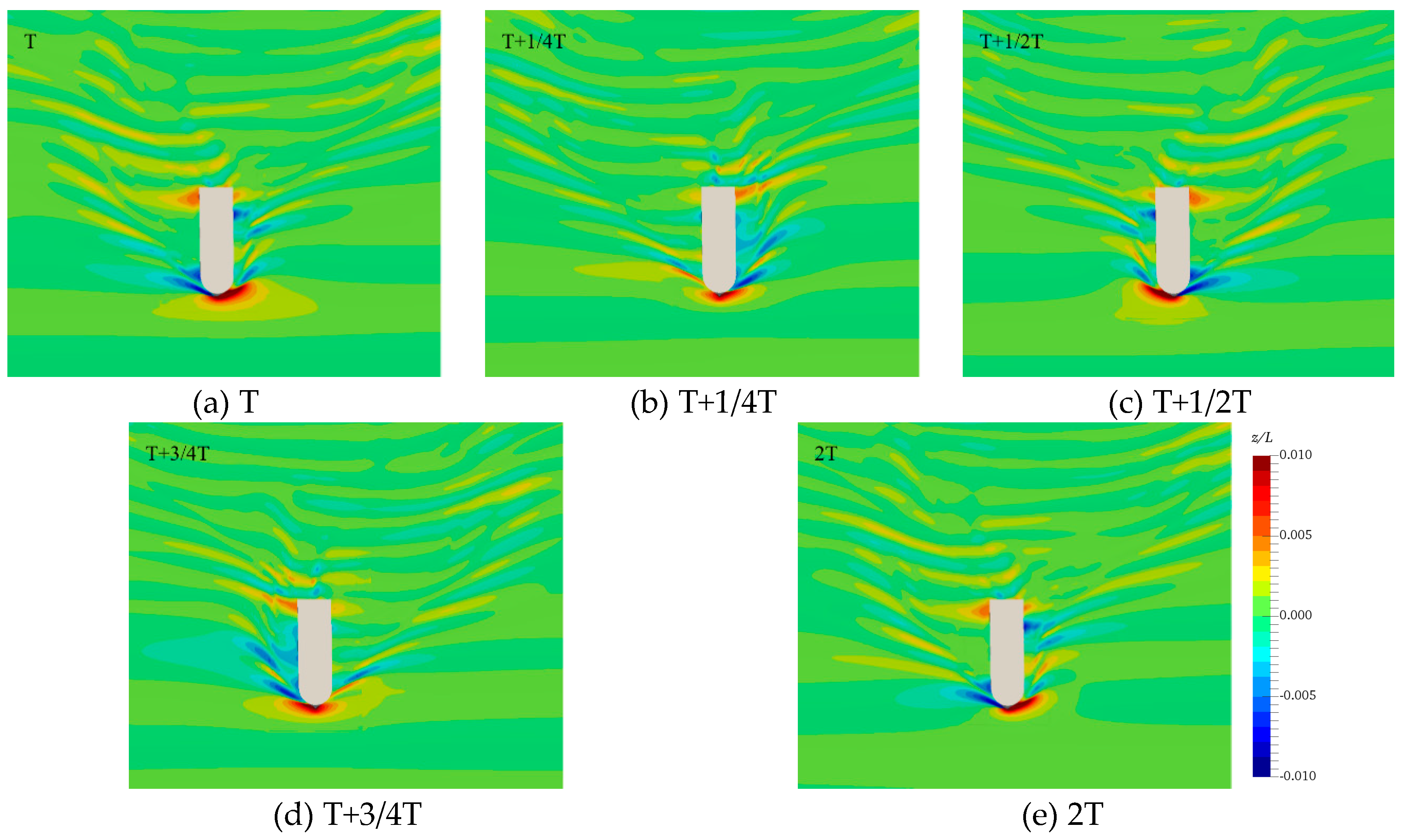
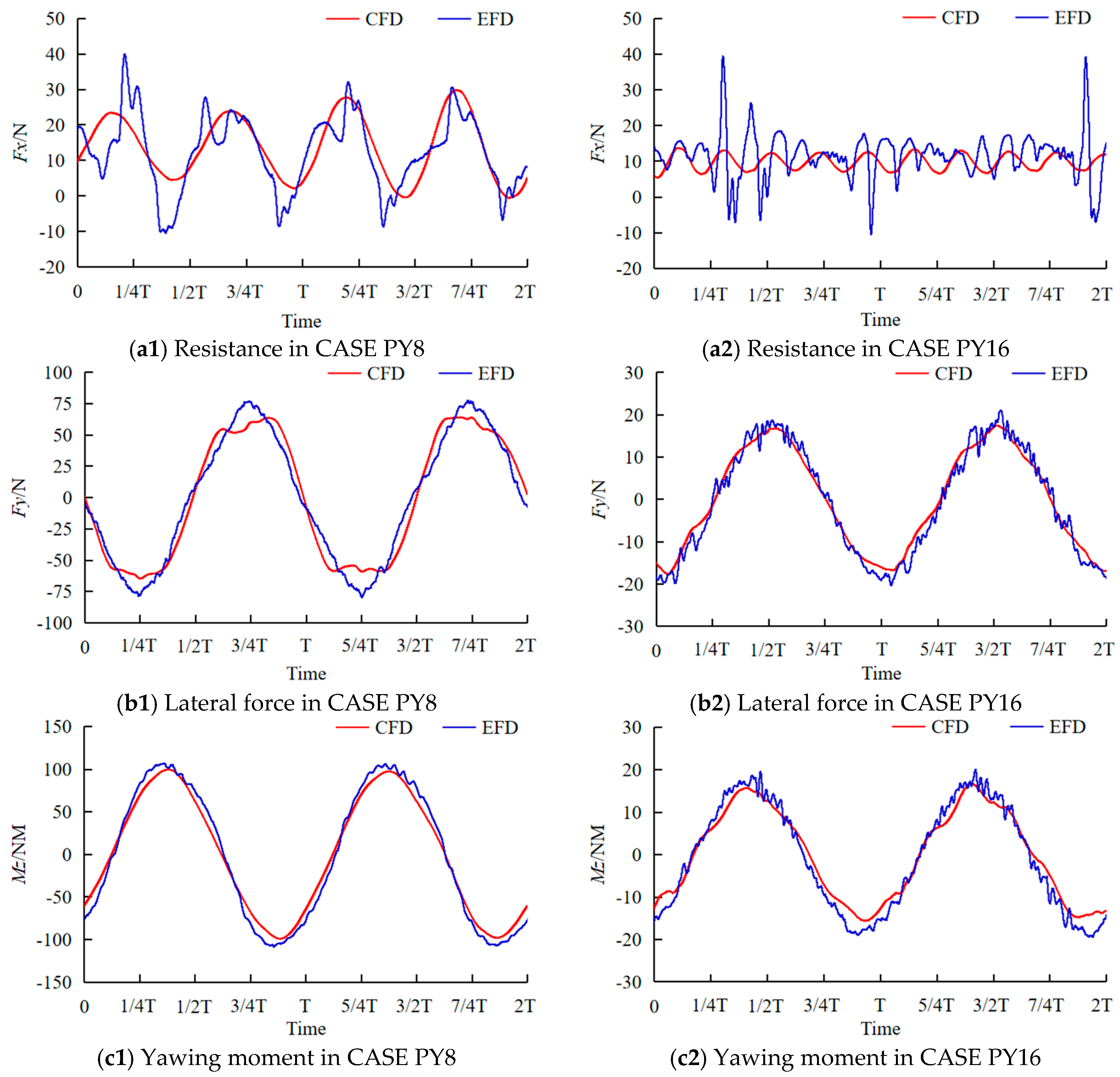
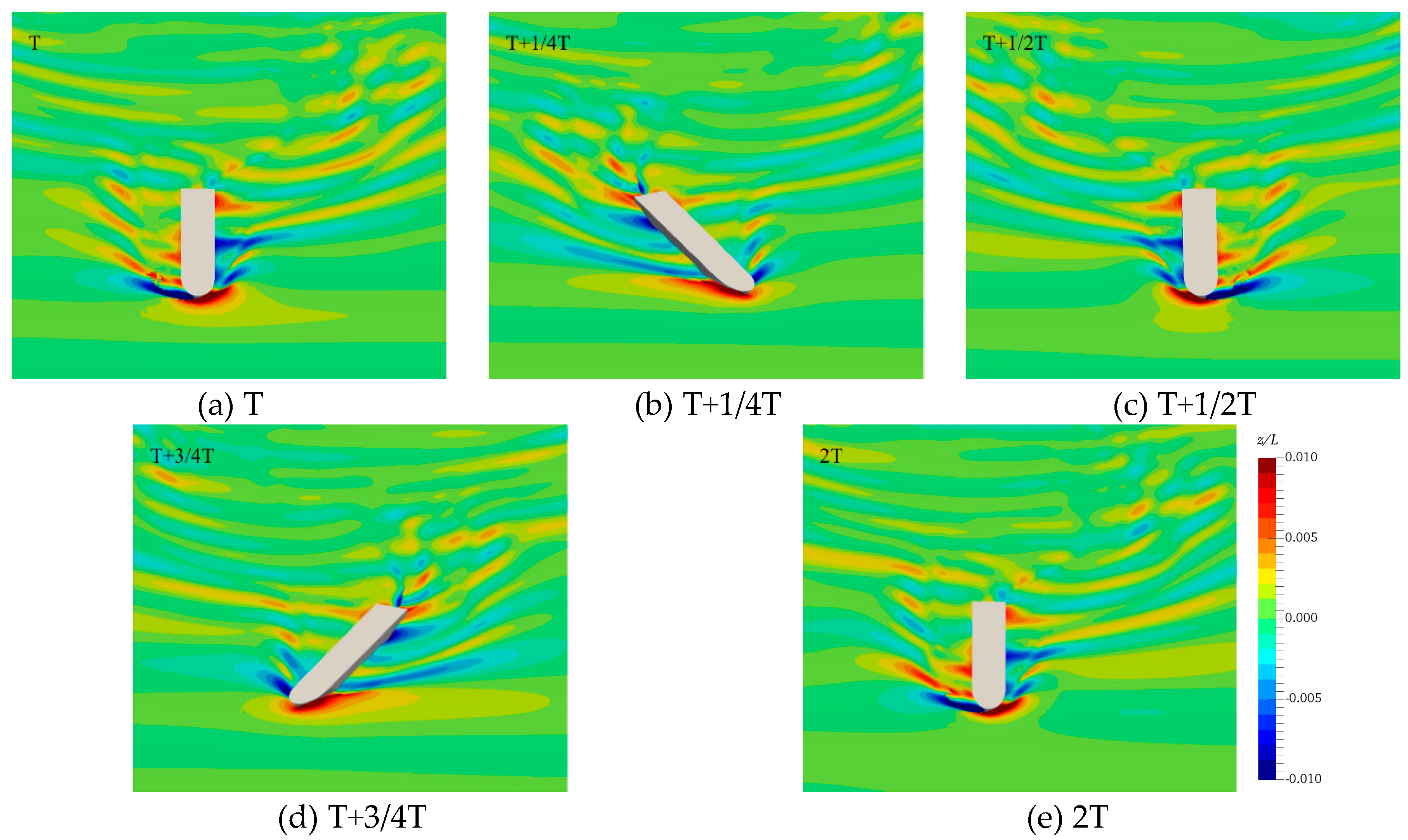
As for the PMM tests, the predicted forces and moments show a good agreement with the experimental data. It indicates that the present numerical schemes are suitable for the simulations of the large separation flow. In the static drift tests, even though the predicted resistance is not accurate enough since there are big fluctuations in the experimental data, the errors of the lateral force and yawing moment are less than 6%. The evolution of the free surface is also captured well and the bow wave breaking is visible at a larger drift angle (CASE DA 20). In the dynamic tests, the shorter period leads to a larger lateral force and yawing moment. In the pure yaw tests, the lateral force in CASE PY16 is only 16.28N, but it increases to 77.28N rapidly when the period is shortened to 8 s. The periodic variation of the lateral force and yawing moment are confirmed by the evolution of the free surface.

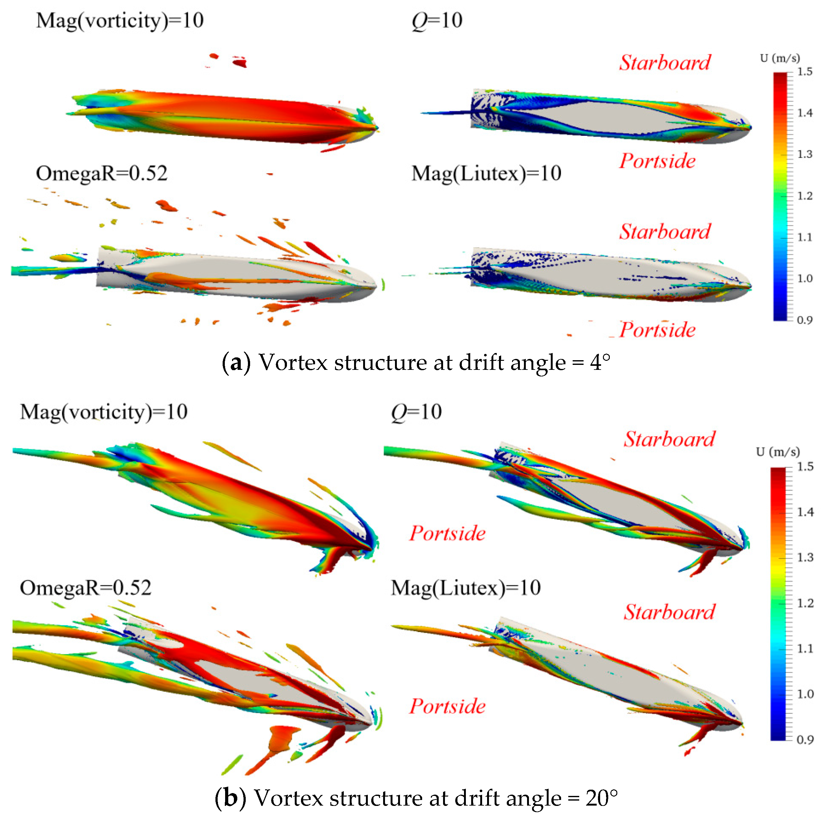
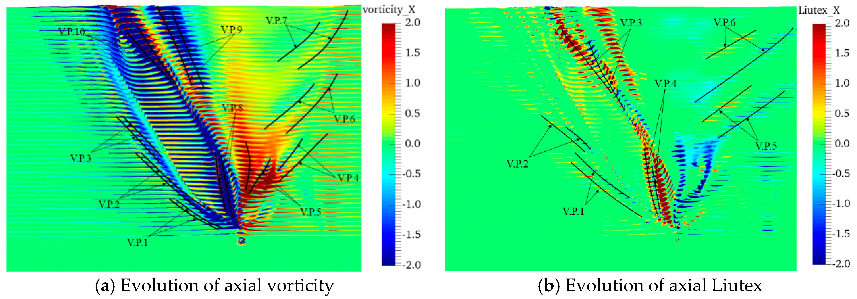
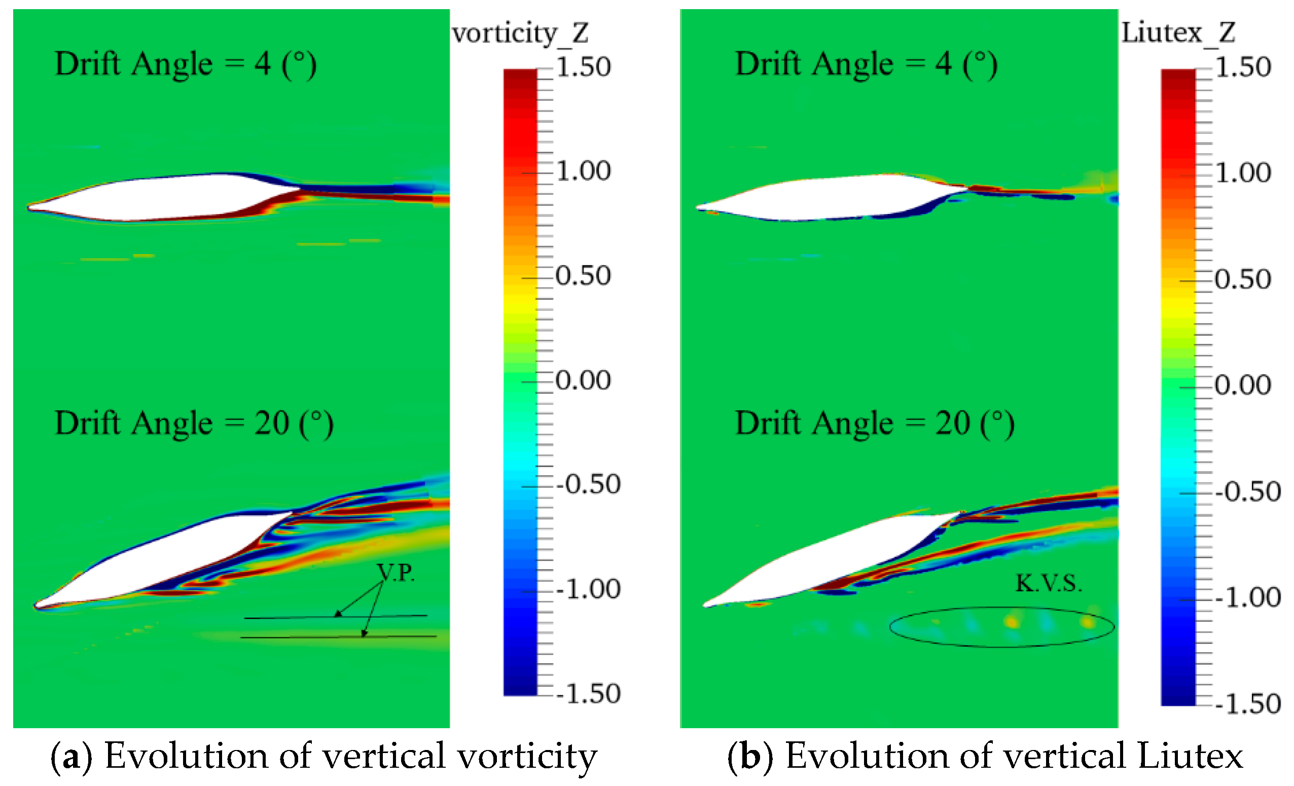
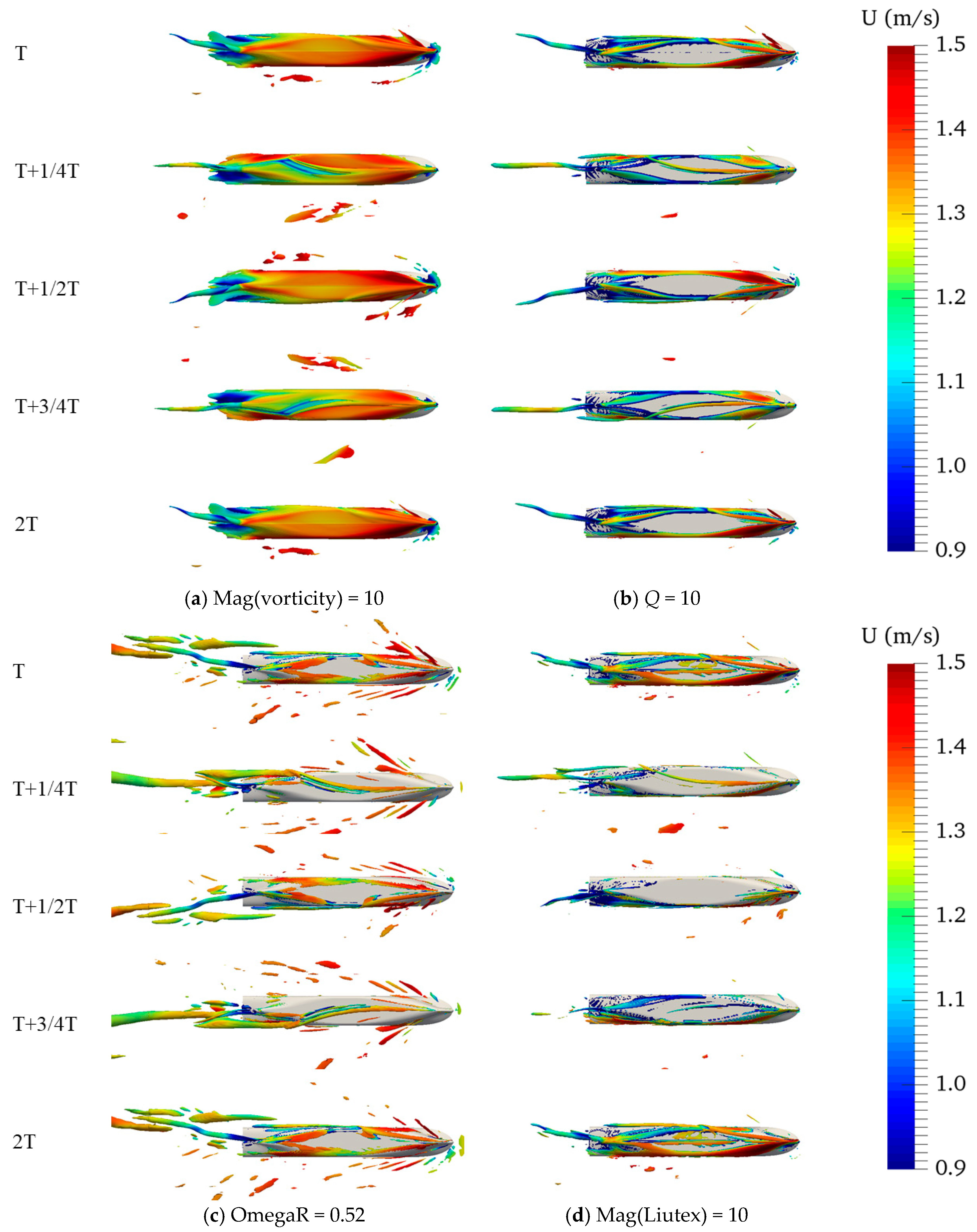
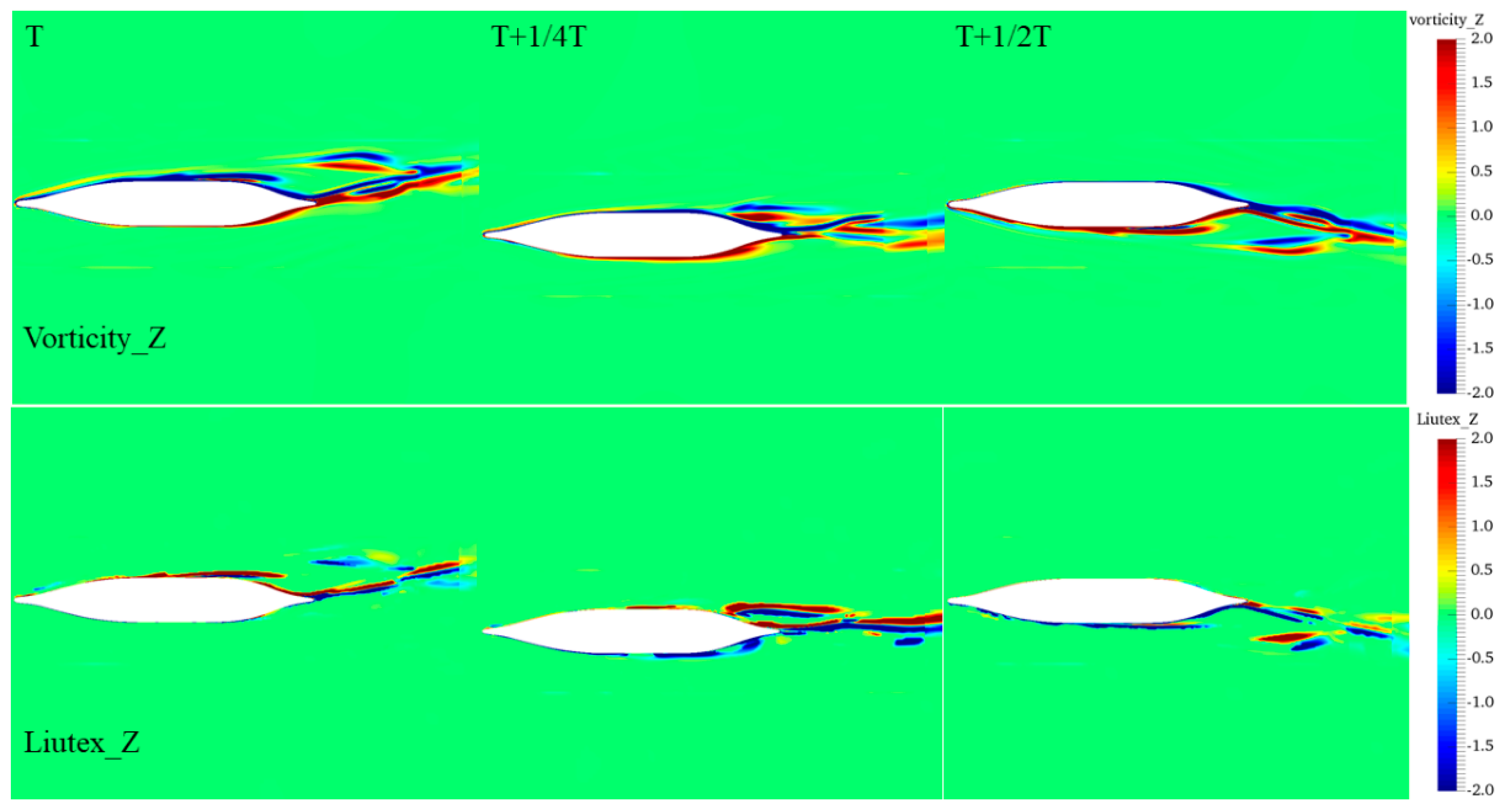
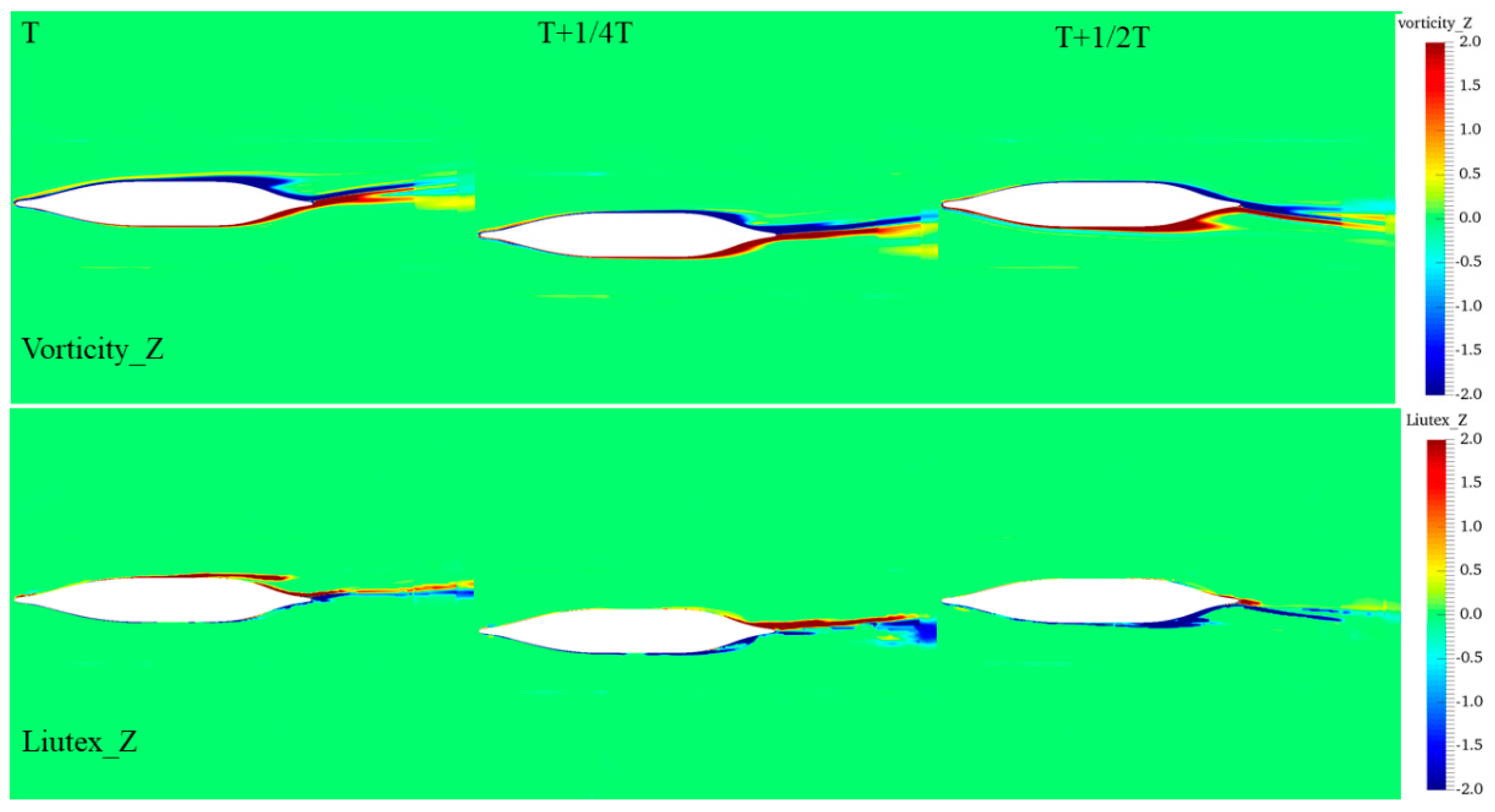
By comparing the vortex structures captured by four vortex identification methods, it is found that the OmegaR method with the insensitive threshold is able to capture more vortex structures in the viscous flows. More breaking and detailed vortex structures are obtained by the Liutex method. The vortex structures obtained by vorticity (first generation) covers the hull fully, which is not reasonable. The Q criterion (second generation) is very sensitive to the artificial threshold. In conclusion, the third generation of vortex identification methods are more suitable for capturing the vortex structures in the large separated flow of the ship.

In the future, DES approaches will be used to solve the viscous flow fields around the ship hull and the results will be compared with the RANS method.

References

1. Tahara, Y.; Longo, J.; Stern, F. Comparison of CFD and EFD for the Series 60 C B = 0.6 in steady drift motion. J. Mar. Sci. Technol. 2002, 7, 17–30. [Google Scholar] [CrossRef]
2. Simonsen, C.D.; Stern, F. Verification and validation of RANS maneuvering simulation of Esso Osaka: Effects of drift and rudder angle on forces and moments. Comput. Fluids 2003, 32, 1325–1356. [Google Scholar] [CrossRef]
3. Pinto-Heredero, A.; Xing, T.; Stern, F. URANS and DES analysis for a Wigley hull at extreme drift angles. J. Mar. Sci. Technol. 2010, 15, 295–315. [Google Scholar] [CrossRef]
4. Ismail, F.; Carrica, P.M.; Xing, T.; Stern, D. Evaluation of linear and nonlinear convection schemes on multidimensional non-orthogonal grids with applications to KVLCC2 tanker. Int. J. Numer. Methods Fluids 2010, 64, 850–886. [Google Scholar] [CrossRef]
5. Xing, T.; Bhushan, S.; Stern, F. Vortical and turbulent structures for KVLCC2 at drift angle 0, 12, and 30 degrees. Ocean Eng. 2012, 55, 23–43. [Google Scholar] [CrossRef]
6. Stern, F.; Agdrup, K.; Kim, S.Y.; Hochbaum, A.C.; Rhee, K.P.; Quadvlieg, F.; Perdon, P.; Hino, T.; Broglia, R.; Gorski, J. Experience from SIMMAN 2008—The First Workshop on Verification and Validation of Ship Maneuvering Simulation Methods. J. Ship Res. 2011, 55, 135–147. [Google Scholar]
7. Meng, Q.J.; Wan, D.C. Numerical simulations of viscous flow around the obliquely towed KVLCC2M model in deep and shallow water. J. Hydrodyn. 2016, 28, 506–518. [Google Scholar] [CrossRef]
8. Wang, J.H.; Liu, X.Y.; Wan, D.C. Numerical Simulation of an Oblique Towed Ship by naoe-FOAM-SJTU Solver. In Proceedings of the 25th International Offshore and Polar Engineering Conference, Big Island, HI, USA, 21–26 June 2015. [Google Scholar]
9. Broglia, R.; Muscari, R.; Di Mascio, A. Numerical simulations of the pure sway and pure yaw motion of the KVLCC-1 and 2 tanker. In Proceedings of the SIMMAN 2008 Workshop on Verification and Validation of Ship Maneuvering Simulation Methods, Lyngby, Denmark, 14–16 April 2008. [Google Scholar]
10. Toxopeus, S.L.; van Walree, F.; Hallmann, R. Maneuvering and Seakeeping Tests for 5415M. In Proceedings of the AVT-189 Specialists’ Meeting, Portsdown West, UK, 12–14 October 2011. [Google Scholar]
11. Cura-Hochbaum, A. On the numerical prediction of the ship’s manoeuvring behaviour. Ship Sci. Technol. 2011, 5, 27–39. [Google Scholar] [CrossRef] [Green Version]
12. Simonsen, C.D.; Stern, F. RANS simulation of the flow around the KCS container ship in pure yaw. In Proceedings of the SIMMAN 2008 Workshop on Verification and Validation of Ship Maneuvering Simulation Methods, Lyngby, Denmark, 14–16 April 2008. [Google Scholar]
13. Sakamoto, N.; Carrica, P.M.; Stern, F. URANS simulations of static and dynamic maneuvering for surface combatant: Part 1. Verification and validation for forces, moment, and hydrodynamic derivatives. J. Mar. Sci. Technol. 2012, 17, 422–445. [Google Scholar] [CrossRef]
14. Sakamoto, N.; Carrica, P.M.; Stern, F. URANS simulations of static and dynamic maneuvering for surface combatant: Part 2. Analysis and validation for local flow characteristics. J. Mar. Sci. Technol. 2012, 17, 446–468. [Google Scholar] [CrossRef]
15. Yoon, H.; Simonsen, C.D.; Benedetti, L.; Longo, J.; Toda, Y.; Stern, F. Benchmark CFD validation data for surface combatant 5415 in PMM maneuvers—Part I: Force/moment/motion measurements. Ocean Eng. 2015, 109, 705–734. [Google Scholar] [CrossRef] [Green Version]
16. Yoon, H.; Longo, J.; Toda, Y.; Stern, F. Benchmark CFD validation data for surface combatant 5415 in PMM maneuvers—Part II: Phase-averaged stereoscopic PIV flow field measurements. Ocean Eng. 2015, 109, 735–750. [Google Scholar] [CrossRef] [Green Version]
17. Kim, H.; Akimoto, H.; Islam, H. Estimation of the hydrodynamic derivatives by RaNS simulation of planar motion mechanism test. Ocean Eng. 2015, 108, 129–139. [Google Scholar] [CrossRef]
18. Yang, Y.; Zou, Z.J.; Zhang, C.X. Calculation of hydrodynamic forces on a KVLCC hull in sway motion in deep and shallow water. Chin. J. Hydrodyn. 2011, 26, 85–93. [Google Scholar]
19. Liu, X.Y.; Fan, S.; Wang, J.H.; Wang, J.; Wan, D. Hydrodynamic Simulation of Pure Sway Tests with Ship Speed and Water Depth Effects. In Proceedings of the 25th International Offshore and Polar Engineering Conference, Big Island, HI, USA, 21–26 June 2015. [Google Scholar]
20. Wang, J.H.; Wan, D.C. Numerical simulation of pure yaw motion using dynamic overset grid technology. Chin. J. Hydrodyn. 2016, 31, 567–574. [Google Scholar]
21. Omer, M.; Chen, X.; Zhou, C.S.; Lunkun, G. Assessment of the modified rotation/curvature correction SST turbulence model for simulating swirling reacting unsteady flows in a solid-fuel ramjet engine. Acta Astronaut. 2016, 129, 241–252. [Google Scholar]
22. Noack, R.W.; Boger, D.A.; Kunz, R.F.; Carrica, P. Suggar++: An improved general overset grid assembly capability. In Proceedings of the 47th AIAA Aerospace Science and Exhibit, San Antonio, TX, USA, 22–25 June 2009; pp. 22–25. [Google Scholar]
23. Liu, C.Q.; Gao, Y.S.; Dong, X.R.; Wang, Y.-Q.; Liu, J.-M.; Zhang, Y.-N.; Cai, X.-S.; Gui, N. Third generation of vortex identification methods: Omega and Liutex/Rortex based systems. J. Hydrodyn. 2019, 31, 205–223. [Google Scholar] [CrossRef]
Figure 1. Geometry model of a Yupeng Ship.
Jmse 08 00649 g001
Figure 2. Computational domain and boundary condition.
Jmse 08 00649 g002
Figure 3. Grid distribution: (a) global grid distribution; (b) grid distribution on the free surface; (c) grid distribution on the hull.
Jmse 08 00649 g003
Figure 4. Grids distributions with different mesh resolutions (top: coarse; middle: mid; bottom: fine).
Jmse 08 00649 g004
Figure 5. Forces and moments in CASE DA4 (left) and DA20 (right) (a: resistance; b: lateral force; c: yawing moment).
Jmse 08 00649 g005aJmse 08 00649 g005b
Figure 6. Free surface: (a) free surface in CASE DA4; (b) free surface in CASE DA20; (c) bow wave in CASE DA20.
Jmse 08 00649 g006aJmse 08 00649 g006b
Figure 7. Dynamic pressure distribution on the hull: (a) dynamic pressure distribution on the portside; (b) dynamic pressure distribution on the starboard side.
Jmse 08 00649 g007
Figure 8. Vortex structure in the simulations of the static drift test: (a) vortex structure in CASE DA4; (b) vortex structure in CASE DA20.
Jmse 08 00649 g008
Figure 9. Evolution of the axial vorticity (a) and Liutex (b) along the ship length direction in CASE DA20.
Jmse 08 00649 g009
Figure 10. Evolution of the vertical vorticity (a) and Liutex (b) at z/Lpp = −0.03572 along the ship length direction in static drift tests (top: CASE DA4; bottom: CASE DA20).
Jmse 08 00649 g010
Figure 11. Forces and moment in CASE PS8 (left) and PS16 (right) (a: resistance; b: lateral force; c: yawing moment).
Jmse 08 00649 g011
Figure 12. Evolution of free surface in one period in CASE PS8.
Jmse 08 00649 g012
Figure 13. Vortex structure obtained by different vortex identification methods: (a) first generation based on vorticity; (b) second generation based on eigenvalues; (c,d) third generation in CASE PS8.
Jmse 08 00649 g013
Figure 14. Vertical vorticity (top) and Liutex (bottom) at z/Lpp = −0.03572 in CASE PS8.
Jmse 08 00649 g014
Figure 15. Vertical vorticity (top) and Liutex (bottom) at z/Lpp = −0.03572 in CASE PS16.
Jmse 08 00649 g015
Figure 16. Forces and moment in CASE PY8 (left) and PY16 (right) (a: resistance; b: lateral force; c: yawing moment).
Jmse 08 00649 g016
Figure 17. Evolution of the free surface in one period in CASE PY8.
Jmse 08 00649 g017
Figure 18. Vortex structures obtained by different vortex identification method: (a) first generation based on vorticity; (b) second generation based on eigenvalues; (c,d) third generation in CASE PY8.
Jmse 08 00649 g018
Figure 19. Vertical vorticity (top) and Liutex (bottom) at z/Lpp = −0.03572 in CASE PY8.
Jmse 08 00649 g019
Figure 20. Vertical vorticity (top) and Liutex (bottom) at z/Lpp = −0.03572 in CASE PY16.
Jmse 08 00649 g020