SPH-FE-Based Numerical Simulation on Dynamic Characteristics of Structure under Water Waves

Abstract

Offshore structures are prone to produce a dynamic response under the effect of large wave load. In this paper, the smoothed particle hydrodynamics coupled with finite element (SPH-FE) method is used to investigate the dynamic characteristics of structure induced by the water waves. The dam break model is assumed to generate water wave. Firstly, the parameter of particle spacing included in the SPH method is examined and the appropriate value is proposed. Subsequently, the present numerical model is validated by comparing with the available results from the literature. Furthermore, the influence of several parameters on the wave load of the structure and the induced dynamic characteristics is studied, including the water column height, the distance between the water column and structure, and the structure stiffness. The results show that the amplification of the wave load on the bottom of structure is greater than that on the upper part of the structure. The increase of structure stiffness results in a decrease in the displacement at the top of structure, but an increase in the hydrodynamic force at the bottom of structure.

1. Introduction

With the development of ocean engineering, a great number of marine structures have been built, for example, wharf, offshore platform, and coastal bridges. Marine structures are prone to produce a large dynamic response when subjected to wave, current, and other hydrodynamic loads [1,2]. Therefore, it is necessary to reasonably predict the wave load on marine structures and the associated dynamic response characteristics.

The wave–structure interaction (WSI) is one of the concerned issues in offshore engineering, for which the sound physical understanding and accurate calculation of WSI are crucial to assess structural responses under waves [3]. The impact of waves on structures is relevant to the issue of fluid–structure interaction (FSI), which refers to the deformation of the structure under the action of the complex free-surface phenomena such as wave surface overturning and breaking. The analytical solutions cannot satisfy the demands of such complicated cases owing to the limitations of the existing mathematical methods [4]. In recent years, with the development of computational fluid dynamics, numerical simulations have been adopted as an alternative tool in the study of the interactions between waves and structures [5,6,7]. The traditional numerical methods, such as finite difference method, finite element method, or boundary element method, are mainly capable of resolving some simple flow problems. However, for some complicated situations with rapid changing of free surface and the induced large deformation of structures, it is still a challenge to reproduce it by numerical modelling.

Recently, mesh-free numerical methods, such as smooth particle hydrodynamics (SPH) [8], have been developed as a promising computational method. For the SPH method, the particles move in Lagrangian coordinates and the advection is directly calculated by particle motion without numerical diffusion [9]. As SPH is a type of mesh-free method, it is inherently suitable for solving the procedures of moving discontinuities with large deformations [3], and it has been utilized to resolve a wide range of hydrodynamics problems [10,11,12,13]. Rafiee et al. [14] used the pressure Poisson equation in the SPH method to solve the incompressible problem of fluid, and verified that the method can well simulate the dynamic response between the free surface of fluid and the structure; Dao et al. [15] established a numerical wave flume based on SPH method, which was successfully applied to simulate the cases of tsunami wave propagating on the slope and wave impacting on coastal structures; and St-Germain et al. [16] used the weak compressibility SPH method to compute the wave force of the rapidly developing tsunami wave acting on the square cylinder, and the computed results fit well with the results of large-scale physical experiments. Although SPH is advantageous for free-surface flow simulations with large deformation, its calculation accuracy and efficiency in simulating small deformation of solid structure are lower than that of the finite element (FE) method. Moreover, there exist tensile instability and difficulty in applying boundary when using SPH to simulate structural dynamics [17,18]. Hence, the pure SPH method is still insufficient to resolve the issue of WSI. Nevertheless, the FE solution can be coupled with SPH to make this method superior. It can not only utilize the advantages of SPH method in simulating complex free surface flow, but also make use of the advantages of high precision and efficiency of the FE method in calculating structural dynamics, thereby, SPH coupled with the FE method (SPH-FE) has been applied in wave–structure simulations [19,20].

In this paper, the SPH-FE method is used to simulate the free-surface flow with large deformation and the synchronously induced dynamic response of structures. Firstly, the classical dam break model is established, and the influence of particle spacing in the SPH method on the simulated results is examined. Subsequently, the feasibility of the present numerical method is verified by comparing with the available results in the literature. Furthermore, several influencing parameters, in terms of the initial wave water column height, distance between water column and structure, as well as stiffness of structure, are systematically analyzed.

2. Governing Equations and Numerical Methods

2.1. SPH Model for Fluid

In the SPH method, the computational domain is discretized into a set of arbitrarily distributed points (or particles), which possess individual material properties (e.g., position, velocity, mass, density, pressure) [16]. Instead of using the traditional computational grid to connect the compute nodes, discrete particles are used to simulate the continuous medium fluid, thus establishing the partial differential equation of fluid motion. The function describing the field Ω is approximated in the form of “kernel function”, which is expressed as the integral form of the product of any function and kernel function [8].

$$<f(x)>={\displaystyle \underset{\mathsf{\Omega }}{\int }f(x\prime )}W(x-x\prime ,h)\mathrm{d}x\prime ,$$

(1)

where x and x’ are the position vectors of two points in the computational domain; f(x) is the continuous function of the field corresponding to the coordinate X; f(x’) is the value of quantity at the point x’; W(x-x’,h) is the smooth kernel function, where h is the smooth length, representing the influence area of the smooth function (i.e., support domain); and h determines the precision and efficiency of the function expression.

For the SPH method, Equation (1) can be rewritten in discretized form of a summation of the neighboring particles in the support domain as follows [8]:

$$<f(x_i)>={\displaystyle \sum _{j=1}^N\frac{m_j}{{\rho }_j}f(x_j)}W(x_i-x_j,h)={\displaystyle \sum _{j=1}^N\frac{m_j}{{\rho }_j}f(x_j)}{W}_{ij},$$

(2)

where i is the number of any particle in the domain; the subscript j is the number of particles close to particle i; N is the total number of particles within the influence area of the particle at x; ρ is the density of fluid particles; and m is the mass of particles.

Substituting the SPH approximations for a function and its derivative to the partial differential equations governing the physics of fluid flows, the discretization of these governing equations can be written as follows [21]:

$$\{\begin{array}{l}\frac{\mathrm{d}{\rho }_i}{\mathrm{d}t}={\displaystyle \sum _j^N{m}_j{v}_{ij}\cdot {\nabla }_i{W}_{ij}}\\ \frac{\mathrm{d}{v}_i{}^{\alpha }}{\mathrm{d}t}={\displaystyle \sum _j^N{m}_j(\frac{{\sigma }_i{}^{\alpha \beta }}{{\rho }_i{}^2}+\frac{{\sigma }_j{}^{\alpha \beta }}{{\rho }_j{}^2}+{\Pi }_{ij})W_{ij,\beta }}+g\\ \frac{\mathrm{d}{e}_i{}^{\alpha }}{\mathrm{d}t}={\displaystyle \sum _j^N{m}_j(v_i{}^{\alpha }-v_j{}^{\alpha })(\frac{{\sigma }_i{}^{\alpha \beta }}{{\rho }_i{}^2}+\frac{1}{2}{\Pi }_{ij})W_{ij,\beta }}\\ \frac{\mathrm{d}{x}_i{}^{\alpha }}{\mathrm{d}t}=v_i{}^{\alpha }+\epsilon {\displaystyle \sum _j^N\frac{m_j}{{\overline{\rho }}_{ij}}{v}_{ji}{W}_{ij}}\end{array},$$

(3)

where the superscripts α and β are the coordinate directions; g is the acceleration of gravity; ε (= 0.5) is the shear strain rate; σ is the particle stress; v is the particle velocity; e is the internal energy per unit mass; and П_ij is the Monaghan artificial viscosity [22], which can convert the kinetic energy of the fluid into heat energy. In the analysis of the interaction between waves and structures, П_ij can prevent the non-physical shock of the solution results in the impact area and effectively prevent the non-physical penetration of particles when they are close to each other. As the smooth kernel function W_ij must be normalized over its support domain and should satisfy the Dirac delta function, the forms of W_ij usually include quantic spline function, cubic spline function, and Gaussian kernel function. By balancing the calculation accuracy and efficiency and considering that this study focuses on two-dimensional problems, the following cubic spline kernel function is adopted:

$$W(x-x\prime ,h)={\alpha }_{\mathrm{D}}\times \{\begin{array}{l}\frac{2}{3}-q^2+\frac{1}{2}{q}^3\begin{array}{cc}& \end{array}\begin{array}{cc}& 0\le q\le 1\end{array}\\ \frac{1}{6}{(2-q)}^3\begin{array}{cccc}& & & \end{array}1\le q\le 2\\ 0\begin{array}{ccc}\begin{array}{cc}\begin{array}{ccc}& & \end{array}& \end{array}& & q\ge 2\end{array}\end{array},$$

(4)

where α_D = 15/7πh²; q = (x − x’)/h.

2.2. Equation of State

When the SPH method is applied in solving the FSI problem, the fluid is treated as weakly compressible, and the pressure of particles is calculated by the density and internal energy of particles through the equation of state, usually in the following form [8]:

$$P=B\left[{\left(\frac{\rho }{{\rho }_0}\right)}^{\gamma }-1\right],$$

(5)

where ρ₀ denotes the reference density and ρ₀ = 1000 kg/m³ for water; γ is a constant, and γ = 7 for water; and B is used to limit the maximum change of pressure, and is usually taken as follows [16]:

$$B=\frac{{\rho }_0{c}_0{}^2}{\gamma },$$

(6)

where c₀ is the artificial speed of sound in water at the reference density. With the increase of c₀, the compressibility of fluid decreases. However, a high value of c₀ may cause the instability of the numerical calculation, and a very small time step is needed at the same time. Therefore, in the numerical simulation, the value of c₀ is often less than the real speed of sound and is generally taken as about 10 times the maximum velocity of the flow field. In that case, the fluid is compressible, but the calculation error is smaller and usually less than 1%, which can satisfy the engineering requirements. Because the maximum velocity is about ${(2g{h}_u)}^{1/2}$ for the dam break model presented in this study, the value of c₀ is $10{(2g{h}_u)}^{1/2}$, where h_u is the height of the initial water column.

2.3. Finite Element Equation for Solid

The FE method based on the updated Lagrangian scheme is currently used to solve the dynamic responses of structures. According to the weighted residual method, the finite element equations of structure motion in the computational domain V can be derived as follows [23]:

$$M_{\mathrm{t}}{a}_{\mathrm{t}}{}^{\alpha }=f_{\mathrm{ext}k}{}^{\alpha }-f_{\mathrm{in}k}{}^{\alpha },$$

(7)

where a_t is the node acceleration; M_t is the node concentrated mass; subscript k is the node number; and f_extk and f_intk are the equivalent external and internal forces acting on node k, respectively, and their expressions are as follows:

$$f_{extk}{}^{\alpha }={\displaystyle \int {}_V{N}_k{\rho }_s{F}_b{}^{\alpha }}\mathrm{d}V+{\displaystyle \int {}_{A_t}{N}_k{F}_t{}^{\alpha }}\mathrm{d}A,$$

(8)

$$f_{\mathrm{int}k}{}^{\alpha }=-{\displaystyle \int {}_V\frac{\partial N_k}{\partial x^{\beta }}}{\sigma }^{\alpha \beta }\mathrm{d}V,$$

(9)

where F_b and F_t represent the physical force and surface force acting on the structure; A_t is the area of F_t; N_k is the finite element shape function of node k; and σ is the stress tensor.

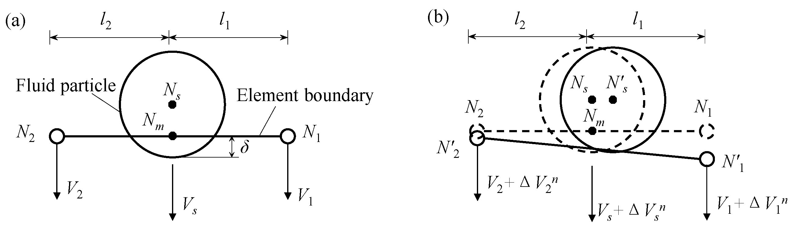
2.4. Fluid–Solid Interface Treatment

As both the FE and SPH methods are based on Lagrangian description, the interface of fluid and structure can be easily handled by contact algorithm. In the present study, the generalized particle algorithm proposed by Johnson [24] is employed to treat the interface between solid element and fluid particle. The particle point is regarded as a node, and the element surface that contacts with the particle point is regarded as the main surface for calculation and processing through contact search.

The contact treatment of fluid and structure is shown in Figure 1, where N₁ and N₂ are two finite element nodes, and the fluid particle N_s is regarded as a sphere with a radius of half of the particle spacing. Before the fluid particles come into contact with the structural nodes, the corresponding velocities of N_s, N₁, and N₂ are V_s, V₁, and V₂ respectively, while l₁ and l₂ are the distances from the center of N_s to N₁ and N₂, respectively. The cross-over distance from fluid particle to structure element is δ, which can be calculated based on the distance from particle center to element boundary and particle radius, as shown in Figure 1a. In order to eliminate interpenetration, the velocity of the fluid particle and structure element node is adjusted through iterative processing of the conservation of momentum and principle of equal velocity at contact points. For instance, during the n-step iteration after the contact between the fluid particle and the structural element, the speed of the corresponding points becomes V_s + ΔV_sⁿ, V₁ + ΔV₁ⁿ, and V₂ + ΔV₂ⁿ, and the positions become N’_s, N’₁, and N’₂, respectively. After the elimination of penetration, the contact point between the fluid and the structure unit is set to N_m, as shown in Figure 1b. The velocity increments ΔV_sⁿ, ΔV₁ⁿ, and ΔV₂ⁿ are calculated by the following equations:

$$\Delta V_{\mathrm{s}}{}^n=\frac{-{\alpha }_{\mathrm{P}}\left(\delta /\Delta t\right)}{1+R_1{}^2{M}_{\mathrm{S}}/M_1+R_2{}^2{M}_{\mathrm{S}}/M_2},$$

(10)

$$\Delta V_1{}^n=-R_1{}^2{M}_{\mathrm{S}}\Delta V_{\mathrm{S}}{}^n/M_1, \Delta V_2{}^n=-R_2{}^2{M}_{\mathrm{S}}\Delta V_{\mathrm{S}}{}^n/M_2,$$

(11)

where M_s, M₁, and M₂ are the masses; R₁(= l₁/l) and R₂ = (l₂/l) are the fractions of momentum transferred from the slave node to the master nodes, where l is the distance from N₁ to N₂; Δt is the integration time increment; and α_P is the penetration adjustment coefficient that determines the fraction of the velocity and position changes during each iteration, ${\alpha }_P=1/\sqrt{N-n+1}$, where N is the total number of iterations and n is the current iteration number.

3. Validation of Numerical Model

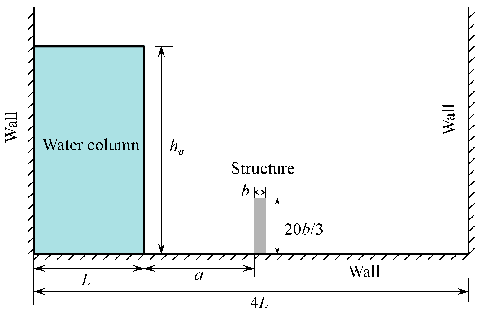
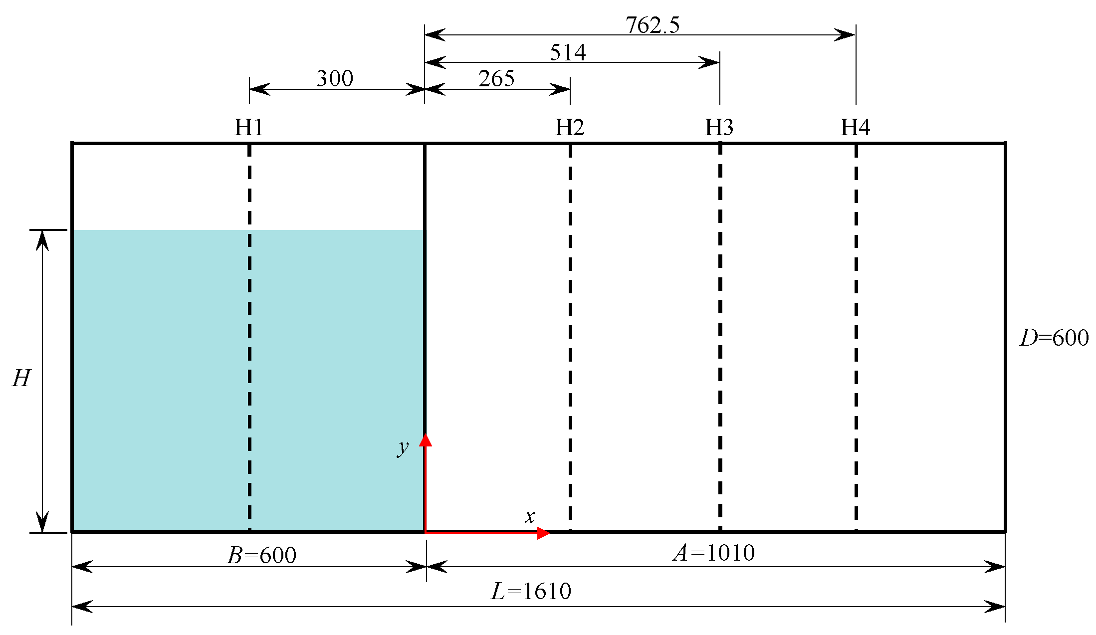
3.1. Computational Case Description

In the classical dam break case, the collapse of water column can generate waves, which is currently used for the numerical simulation of the wave–structure interaction problem in this study. Chanson [25] compared the tsunami surge caused by the Indian Ocean earthquake in 2004 with the dam-break wave, and demonstrated that the flow characteristics of the two waves are very similar. The dam break is a classical experiment that has been widely reported in the literature [26,27,28,29] and has also been used to validate numerical models [30,31]. In the process of dam break, the deformation of free surface is very large and complex. Specifically, when the water hits the wall, the water surface will break and roll over, and the induced structure dynamic response is significant, which can be used to model the waves impacting the marine structures.

The initial setup of the numerical model is shown as Figure 2, where h_u and L are the height and the width of water column, respectively; b is the width of structure, and the height of structure is 20b/3; and a is the distance between water column and structure. At the initial stage, the water column is located on the left side of the fixed wall of the rectangular tank with a length of 4 L and keeps a static equilibrium state. The bottom of the structure is consolidated with the tank. The water column is released at the time of t = 0 to collapse under the action of gravity, generating a dam break wave impacting the structure.

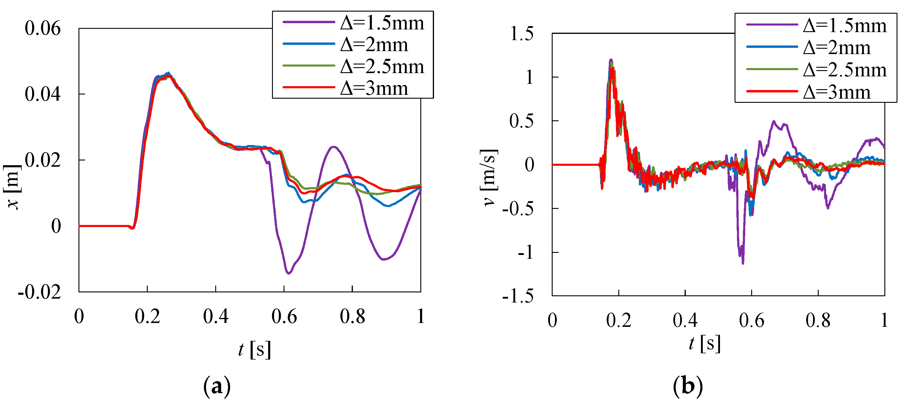
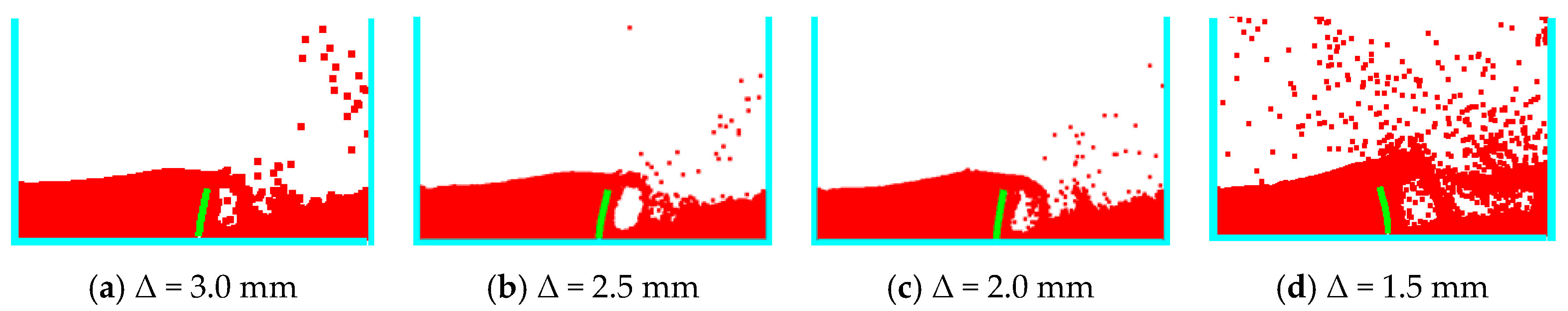
3.2. The Effect of SPH Particle Spacing

In the SPH method, the fluid particles are uniformly arranged, and the neighboring particles in the support domain are continuously searched in the computation process. The initial smooth length h determines the area of influence by the particles, which results in a different total mass of neighbor particles searched, and finally affects the numerical results. The initial particle spacing Δ is an important parameter to determine the smooth length h, and the relationship between the two is as follows [16]:

$$h=0.725{(3{\Delta }^2)}^{1/2}$$

(12)

Properly reducing the initial particle spacing can improve the accuracy of calculation, but too small particle spacing will lead to the instability of computation [32]. In this study, the water fluid deformation is solved by the SPH method. We first investigated the influence of different initial particle spacing Δ on the computed results. The adopted four initial particle spacings and the corresponding total number of particles are shown in

Table 1. Parameters of particle spacing.

Test No.	Initial Particle Spacing Δ [mm]	Number of Particles
1	3.0	4753
2	2.5	6786
3	2.0	10,658
4	1.5	18,915

. The geometry model settings are h_u = 25.2 cm, L = 14.6 cm, a = 14.6 cm, and b = 1.2 cm. The structure is made of sub elastic material, with the density of ρ_s = 2500 kg/m³ and Young’s modulus of E = 10⁶ N/m², which is solved by the FE method with the minimum element of 0.002 m. As the SPH is based on the weakly compressible model, the time step Δt should satisfy the CFL (Courant-Friedrichs-Lewy number) condition [33]:

$$\frac{\Delta t\cdot c}{\Delta }\le 0.2$$

(13)

where c is the speed of sound.

Figure 3 presents the computed horizontal displacement x and velocity v at the top of the structure using different particle spacings. It can be seen that the maximum displacement and velocity of the structure occur at t = 0.25 s and t = 0.187 s, respectively. A comparison of the results with different initial particle numbers shows that the displacement and velocity of the structure are generally same when t < 0.5 s, whereas the computed results are clearly different when t > 0.5 s. When Δ = 2.0 mm~3.0 mm, the computed results tend to be overlapped. However, for the case of Δ = 1.5 mm, the time histories of displacement and velocity fluctuate greatly, and the free surface profile of fluid with Δ = 1.5 mm is quite different from those with Δ = 2.0~3.0 mm. Figure 4 shows the free surface shape of the fluid and the induced deformation of the structure and at the moment of t = 0.62 s. It is observed that, when Δ = 1.5 mm (i.e., small particle spacing and large number of particles), water splash is more obvious. For this case, there are too many particles in the support domain of the kernel function, which causes the viscosity of the fluid to decrease and the shear modulus is correspondingly decreased, hence the computed free surface deformation is too large. This is consistent with previous relevant studies that the smaller particle spacing leads to the smaller stiffness and the larger deformation [34]. Combining the numerical accuracy and calculation efficiency, the particle spacing of Δ = 2.5 mm is selected for the subsequent simulation.

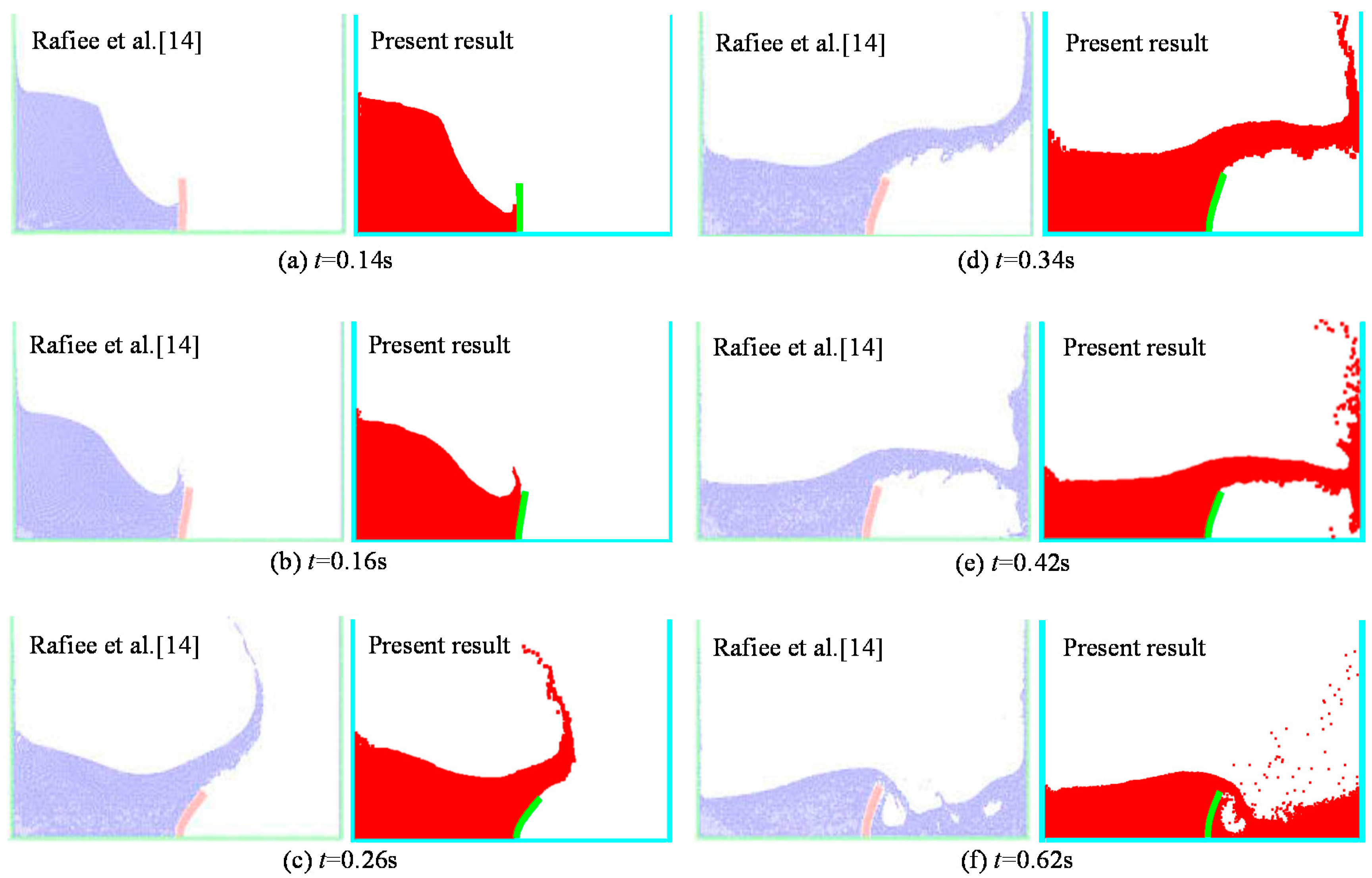
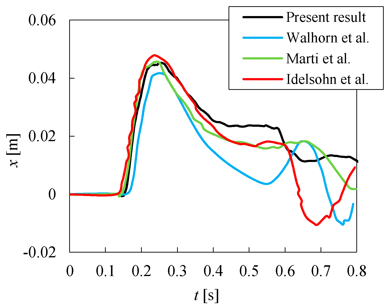
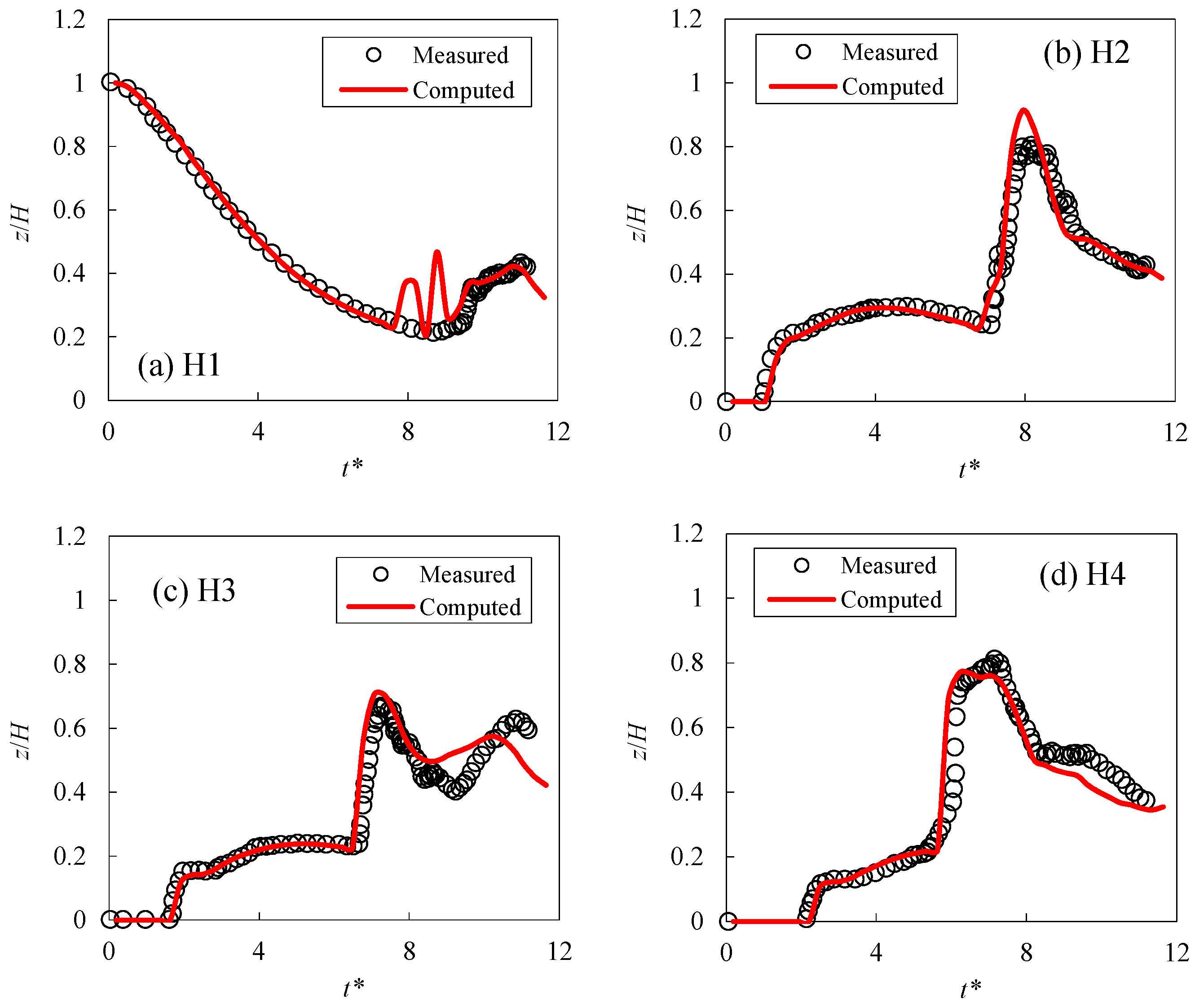
3.3. Model Verification

In order to verify the feasibility of the model, the results of structural deformation and free surface shape at different times are compared with those obtained by particle finite element (PFE) [14], as shown in Figure 5. It can be seen that both the water fluid movement and the structure deformation simulated by the present SPH-FE method are in good agreement with the results by PFE. At the initial moment, the water column collapses, and the fluid flows forward to hit the structure. When t = 0.14 s, the fluid reaches the position of the structure, and starts to rises along the left side of the structure. After that, the water continues to climb and overtops the structure when t = 0.26 s. The free surface of the fluid deforms violently and water splashing occurs; meanwhile, the structure experiences deflection. When t = 0.34 s, the water moves forward and impacts the right side of the tank. Finally, the fluid falls back to the bottom of the tank along the right wall, resulting in free surface fusion.

In addition, the time history of the displacement of the upper left corner of the structure is also compared with other available numerical results [5,6,7] and is illustrated in Figure 6. It can be seen that, in the early stage of the simulation, the results calculated by the present SPH-FE method are consistent with the results in the literature. The peak value of the displacement as well as the corresponding time fit well with the other results. It is worth noting that some differences are found for the different method at the later stage owing to the complex free surface fusion process. However, the present study is mainly focused on the arrival time of waves and the peak displacement of the structure during the early stage. Hence, the SPH-FE method adopted here is feasible for the present study. To further validate the present model, the additional comparison with classical dam-break case by experiment is included in the Appendix A.

4. Analysis of Wave–Structure Interaction

In this study, a series of numerical experiments for the case of dam break wave impacting the structure were conducted to investigate the effects of several parameters on wave arrival time, wave load characteristics, and structure response. The influential parameters include the height of water column h_u, the distance between water column and structure a, and the stiffness of structure E. The conditions for the total cases are listed in

Table 2. Calculation conditions.

Test No.	hu [mm]	a [mm]	E [kPa]
1	292	146	3.0 × 107
2	252	146	3.0 × 107
3	332	146	3.0 × 107
4	292	176	3.0 × 107
5	292	206	3.0 × 107
6	292	146	1.5 × 107
7	292	146	7.5 × 106

. The width of water column L is set as 146 mm for all the cases.

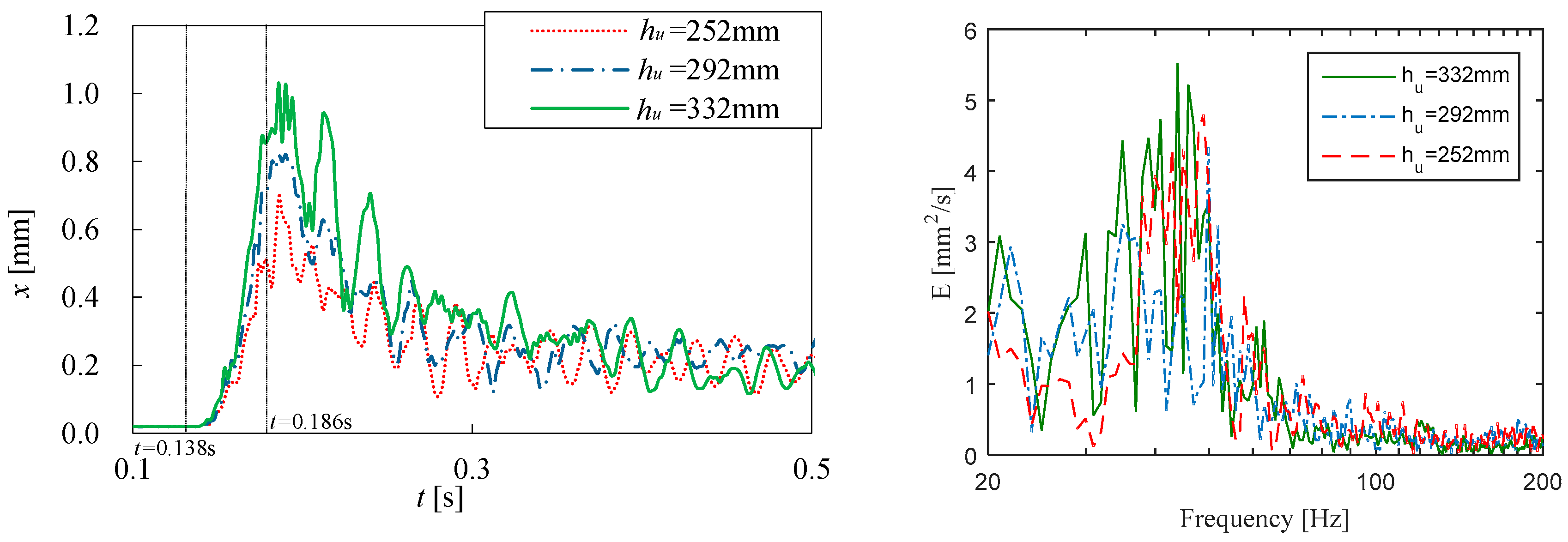
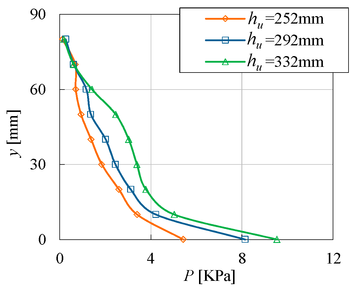
4.1. Effect of Water Column Height

Figure 7 presents the horizontal displacements at the upper left corner of the elastic structure for different water column height. It illustrates that water waves reach the structure at t = 0.138 s under different water column heights. The influence of water column height on the arrival time of water wave is not noticeable. When t = 0.186 s, the displacement of the structure reaches the peak value, and the response duration of the structure from the beginning of movement to the peak value is very short (i.e., 0.048 s). The peak value of the displacement is expected to increase with the increase of the water column height. The displacement amplitude of the structure decreases rapidly with time and decays to approximately 30% of the peak value after t = 0.3 s. Additionally, it can be seen from the curve shape that the displacement of the structure exhibits the characteristics of simple harmonic vibration under the impact of the fluid, and the attenuation of residual vibration is slow. In order to assess the periodicity and verify the appearance of super-harmonics of the structure vibration, the spectral analysis was also conducted using fast Fourier transformation (FFT) of time-series data. The corresponding results are plotted at the right of Figure 7. As can be seen, the peak frequency for all the cases is approximately within the range of 40–50 Hz, which is related to the natural frequency of the structure.

Figure 8 shows the vertical distribution of the extreme pressure P on the structure. The maximum wave pressure appears at the bottom of the structure regardless of the water column height. The peak pressure along the wave front of the whole structure increases with the increase of the water column height, which is reasonable because the higher water column with larger potential energy will result in larger wave load on the structure. The large pressure is confined near the bottom of the structure (y < 10 mm), which indicates that the bottom of the structure is greatly impacted by the water wave. The reason is that the collapsed water wave first arrives at the bottom part of the structure with large energy; subsequently, the water climbs on the structure with water splashing and energy dissipation. Hence, the wave-induced pressure on the bottom is comparatively larger owing to stronger water particle impacting on the bottom of the structure.

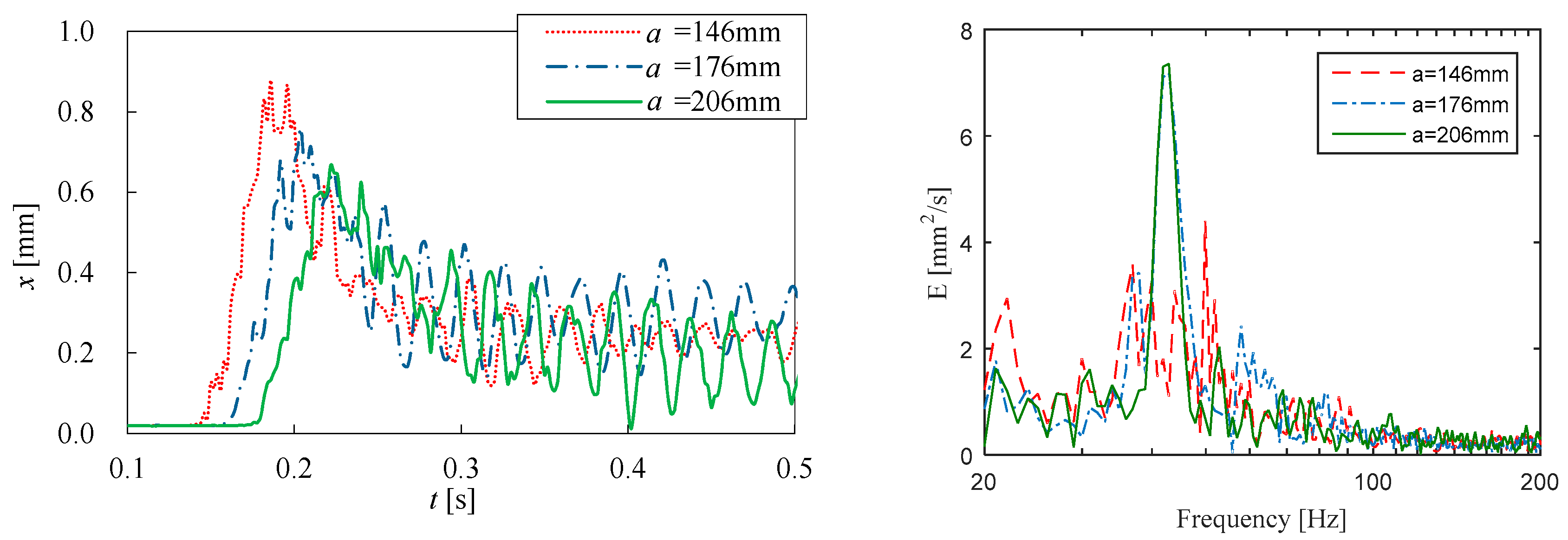
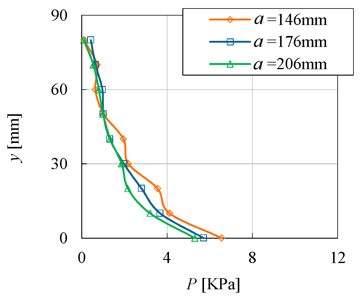
4.2. Effect of Distance between Water Column and Structure

Figure 9 and Figure 10 show the time history of horizontal displacement at the top of structure and the vertical distribution of the extreme pressure on the structure, respectively. It demonstrates that, with the increase of water–structure spacing, the starting time of structure movement is expected to occur later. The corresponding maximum displacements at the top of the structure are 0.82 mm, 0.76 mm, and 0.67 mm for the cases of a = 146 mm, a = 176 mm, and a = 206 mm, respectively, which indicates that the maximum displacement decreases with the increase of a. This can be explained that the hydrodynamic energy of the incident waves is gradually diffused in the propagating process, and thus longer distance results in more energy diffusion and the induced structure response is correspondingly weakened. However, the response duration of the structure from the beginning of movement to the peak value is almost equal. The frequency spectrum analysis at the right of the figure illustrates that the peak frequency is more significant as the distance between the structure and the water column is increased. This can be explained in that the solitary wave generated by the collapsed water is more fully developed with a longer distance, which causes the structural vibration under the water waves to behave more periodically. Figure 10 indicates that the extreme pressure P decreases slightly with the increase of a, and the difference is more obvious near the bottom of the structure.

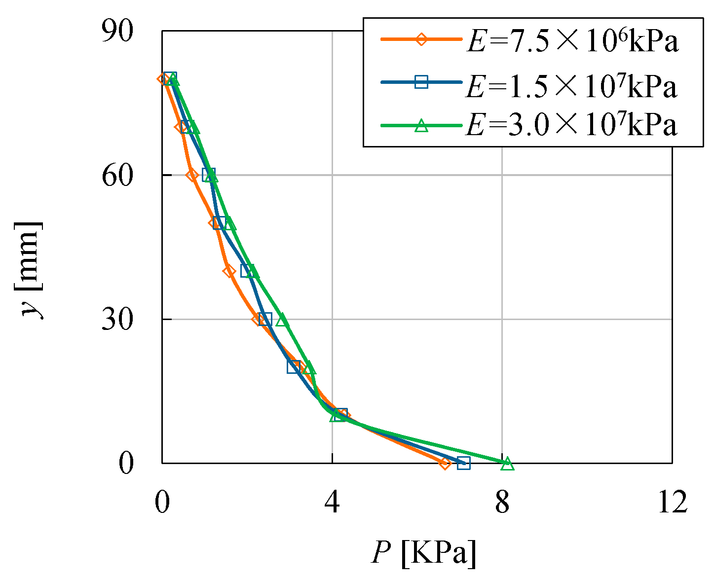
4.3. Effect of the Structure Stiffness

The displacement at the top of the structure with different Young’s modulus E is plotted in Figure 11. With the decrease of the structure stiffness (i.e., increasing the value of Young’s modulus), the starting time for the structure movement remains almost the same, whereas the time corresponding to the peak value of the displacement is delayed, which indicates that the response time of the structure increases. The amplitude of displacement increases with the decrease of the structure stiffness, as expected. The frequency spectrum analysis illustrates that the peak frequency increases with the increase of structural stiffness, as can be seen from the circle plotted in the figure. Overall, the effect of structure stiffness on the dynamic response of structure is significant, including both the displacement and the frequency of the vibration, and this phenomenon is reasonably reproduced by the present numerical modeling.

Figure 12 shows the vertical distribution of the wave pressure P on the structure under different structure stiffness. With the increase of the stiffness of the structure, the peak value of the wave pressure increases slightly. This is consistent with the finding by Sriram et al. [11], who pointed out that the wave pressure of the rigid wall is 1.125 times of that of the elastic wall. Compared with the structure with larger stiffness, the structure with smaller stiffness absorbs more fluid momentum and transforms it into structure deformation, thus its surface pressure is relatively smaller.

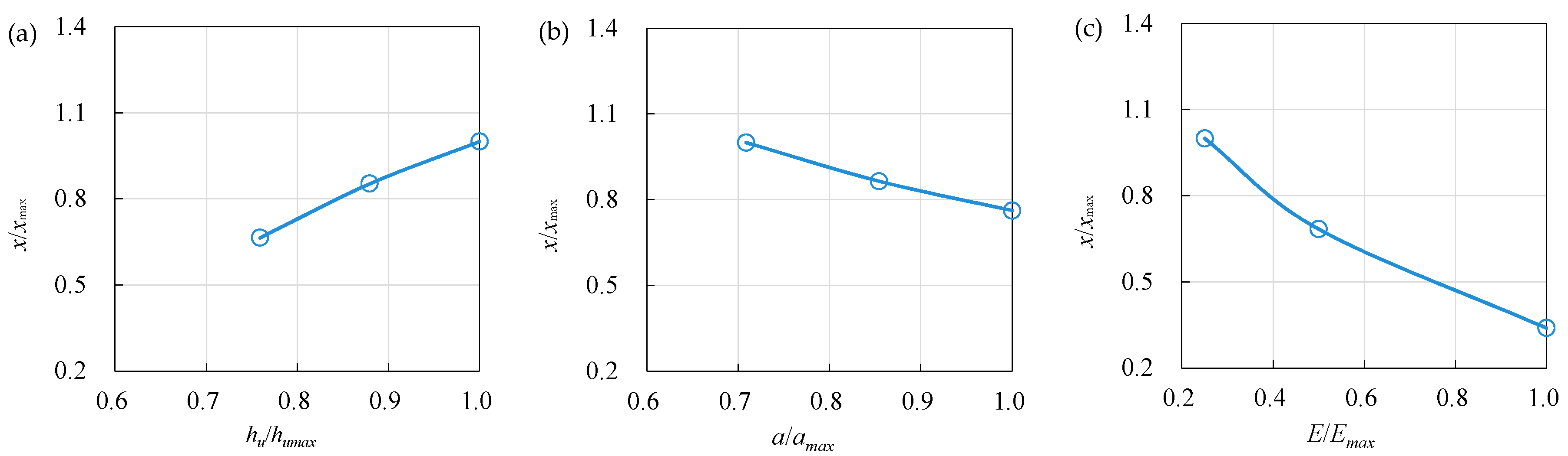
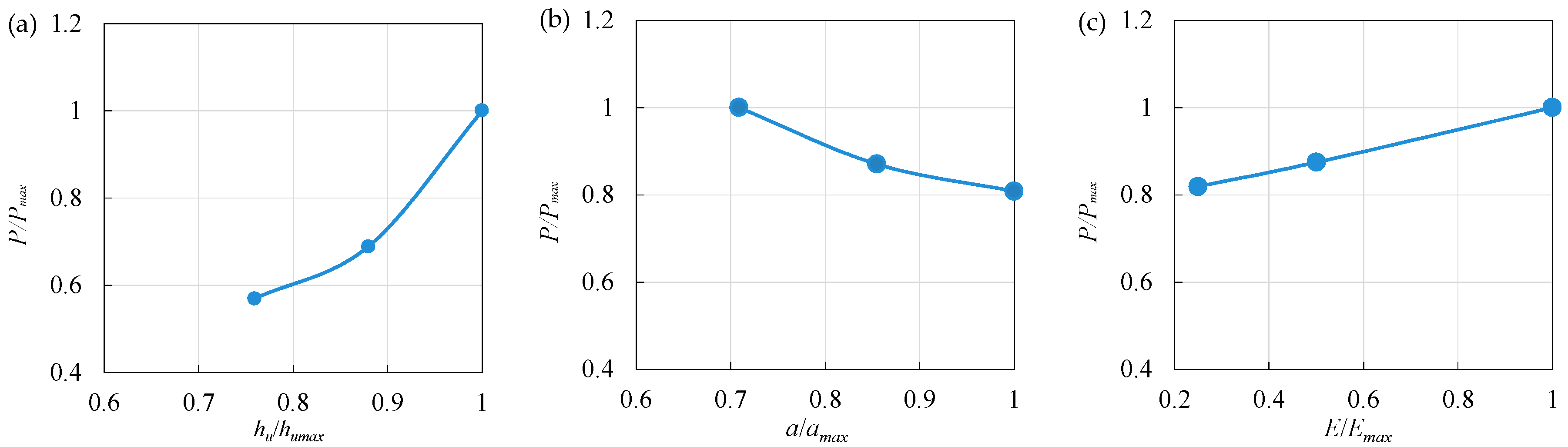
4.4. Comprehensive Analysis

In this section, the influence of the above-mentioned parameters (i.e., the height of the water column h_u, the distance between the water column and the structure a, and the Young’s modulus E) on the structure displacement x and pressure P_b is comprehensively analyzed, as illustrated in Figure 13 and Figure 14, respectively. In the figures, the variable is normalized by its maximum value. Figure 13 indicates that x/x_max is increased with increasing h_u/h_umax, but decreased with increasing a/a_max and E/E_max. Figure 14 shows that P/P_max is increased with increasing h_u/h_umax and E/E_max, but decreased with increasing a/a_max. The reason has been mentioned above, that is, the higher water column means more potential energy of the water, and thus the hydrodynamic force impacting the structure is comparatively larger, inducing larger deformation of structure. The effect of a is mainly reflected from the energy diffusion during the collapsed water wave propagating to the structure, that is, a longer distance means more energy diffusion and relatively less kinetic energy acting on the structure, and the resultant smaller hydrodynamic force and structural displacement. Smaller stiffness implies that the structure deformation will be larger subjected to the same external force. Whereas the structure deformation in turn affects the hydrodynamic load on the structure, because this is an interaction process. The structure with larger deformation absorbs more fluid momentum and transforms it into structure deformation, thus its hydrodynamic load is relatively smaller.

In addition, by combining Figure 13 and Figure 14, it can be seen that, when h_u/h_umax is increased by 0.3, the value of x/x_max is increased by about 0.4, and P/P_max by 0.5. When a/a_max is increased by 0.3, the value of x/x_max is decreased by about 0.3. Therefore, compared with the distance between the water column and the structure, the wave hydrodynamic effect caused by the change of the height of the water column is more pronounced. In addition, when E/E_max is increased by 0.8, the value of x/x_max is reduced by about 0.7, and P/P_max is increased only by about 0.2. It is suggested that the effect of the structure stiffness on the displacement of the structure is comparatively greater than that of the pressure on the structure. In other words, the natural parameter for the structure is more significant compared with the external condition, for example, hydrodynamic force. In the present study, only the stiffness is considered, and further research needs to be conducted to explore the effects of other structural parameters on the dynamic response behavior.

5. Summary and Conclusions

In this study, the SPH-FE coupling method was presented to numerically investigate the dynamic characteristics of structure under dam-break waves, mainly focusing on the displacement at the top of structure. The influence of SPH particle spacing on the numerical results was firstly analyzed, and the model was validated by comparing with previous experimental and numerical results in terms of water surface elevation and structure vibration. The verified numerical model was further applied to investigate the effects of several parameters including the height of water column h_u, the distance between water column and structure a, and the stiffness of structure E.

The validation with dam break case indicates that the present SPH method can accurately predict the water surface elevation. The structure vibration under the impact of dam-break wave, especially the displacement of structure, can be reasonably simulated by the numerical model. The initial particle spacing Δ is a key parameter in the SPH simulation, which needs to be calibrated carefully. The present results show that Δ = 2.5 mm is the appropriate value considering both the computational accuracy and numerical stability.

The parametric analysis illustrates that the structure displacement is increased with increasing h_u, but decreased with increasing a and E. The hydrodynamic force is increased with increasing h_u and E, but decreased with increasing a. The frequency spectral analysis clearly demonstrates the periodic behavior of the structure vibration. The peak frequency is significant for all cases and is mainly influenced by the stiffness of the structure.

References

1. Cuomo, G.; Allsop, W.; Bruce, T.; Pearson, J. Breaking wave loads at vertical seawalls and breakwaters. Coast. Eng. 2010, 57, 424–439. [Google Scholar] [CrossRef] [Green Version]
2. Hsiao, S.C.; Lin, T.C. Tsunami-like solitary waves impinging and overtopping an impermeable seawall: Experiment and RANS modeling. Coast. Eng. 2010, 57, 1–18. [Google Scholar] [CrossRef]
3. Liu, X.; Xu, H.H.; Shao, S.D.; Lin, P.Z. An improved incompressible SPH model for simulation of wave-structure interaction. Comput. Fluids 2013, 71, 113–123. [Google Scholar] [CrossRef]
4. Ni, X.; Feng, W.B.; Wu, D. Numerical simulations of wave interactions with vertical wave barriers using the SPH method. Int. J. Numer. Methods Fluid. 2014, 76, 223–245. [Google Scholar] [CrossRef]
5. Walhorn, E.; Kölke, A.; Hübner, B.; Dinkler, D. Fluid–structure coupling within a monolithic model involving free surface flows. Comput. Struct. 2005, 83, 2100–2111. [Google Scholar] [CrossRef]
6. Marti, J.; Idelsohn, S.; Limache, A.; Calvo, N.; D’Elía, J. A fully coupled particle method for quasi incompressible fluid-hypoelastic structure interactions. Mecánica Comput. 2006, XXV, 809–827. [Google Scholar]
7. Idelsohn, S.R.; Marti, J.; Limache, A.; Oñate, E. Unified Lagrangian formulation forelastic solids and incompressible fluids: Application to fluid structure interaction problems via the PFEM. Comput. Methods Appl. Mech. Eng. 2008, 197, 1762–1776. [Google Scholar] [CrossRef]
8. Monaghan, J.J. Simulating free surface flows with SPH. J. Comput. Phys. 1994, 110, 399–406. [Google Scholar] [CrossRef]
9. Lo, E.Y.M.; Shao, S.D. Simulation of near-shore solitary wave mechanics by an incompressible SPH method. Appl. Ocean Res. 2002, 24, 275–286. [Google Scholar]
10. Sriram, V.; Ma, Q.W. Improved MLPG_R method for simulating 2D interaction between violent waves and elastic structures. J. Comput. Phys. 2012, 231, 7650–7670. [Google Scholar] [CrossRef]
11. Liu, M.B.; Liu, G.R. Smoothed Particle Hydrodynamics (SPH): An overview and recent developments. Arch. Comput. Methods Eng. 2010, 17, 25–76. [Google Scholar] [CrossRef] [Green Version]
12. Liu, H.X.; Li, J.; Shao, S.D.; Tan, S.K. SPH modeling of tidal bore scenarios. Nat. Hazards 2015, 75, 1247–1270. [Google Scholar] [CrossRef] [Green Version]
13. St-Germain, P.; Nistor, L.; Townsend, R. Numerical Modeling of Tsunami-Induced Hydrodynamic Forces on Onshore Structures Using SPH. In Proceedings of the 33rd International Conference on Coastal Engineering (ICCE), Santander, Spain, 1–6 July 2012; pp. 1–15. [Google Scholar]
14. Rafiee, A.; Thiagarajan, K.P. An SPH projection method for simulating fluid-hypoelastic structure interaction. Comput. Methods Appl. Mech. Engrg. 2009, 198, 2785–2795. [Google Scholar] [CrossRef]
15. Dao, M.H.; Xu, H.; Chan, E.S.; Tkalich, P. Modelling of tsunami-like wave run-up, breaking and impact on a vertical wall by SPH method. Nat. Hazards Earth Syst. Sci. 2013, 13, 3457–3467. [Google Scholar] [CrossRef]
16. St-Germain, P.; Nistor, L.; Townsend, R.; Shibayama, T. Smoothed-Particle hydrodynamics numerical modeling of structures impacted by tsunami bores. J. Waterw. Port Coast. Ocean Eng. 2014, 140, 66–81. [Google Scholar] [CrossRef]
17. Vuyst, T.D.; Vignjevic, R.; Campbell, J.C. Coupling between meshless and finite element methods. Int. J. Impact Eng. 2005, 31, 1054–1064. [Google Scholar] [CrossRef]
18. Groenenboom, P.H.L.; Cartwright, B.K. Hydrodynamics and fluid-structure interaction by coupled SPH-FE method. J. Hydraul. Res. 2010, 48, 61–73. [Google Scholar] [CrossRef]
19. Hu, D.A.; Long, T.; Xiao, Y.H.; Han, X.; Gu, Y.T. Fluid-structure interaction analysis by coupled FE-SPH model based on a novel searching algorithm. Comput. Methods Appl. Mech. Eng. 2014, 276, 266–286. [Google Scholar] [CrossRef] [Green Version]
20. Thiyahuddin, M.I.; Gu, Y.T.; Gover, R.B.; Thambiratnam, D.P. Fluid-structure interaction analysis of full scale vehicle-barrier impact using coupled SPH-FEA. Eng. Anal. Bound. Elem. 2013, 42, 26–36. [Google Scholar] [CrossRef] [Green Version]
21. Petsehek, A.C.; Libersky, L.D. Cylindrical smoothed particle hydrodynamies. J. Comput. Phys. 1993, 109, 76–80. [Google Scholar] [CrossRef]
22. Monaghan, J.J. Smoothed particle hydrodynamics. Annu. Rev. Astron. Astrophys. 1992, 30, 543–574. [Google Scholar] [CrossRef]
23. Xiao, Y.H.; Han, X.; Hu, D.A. FE-SPH coupling simulation of fluid structure interaction. Chin. J. Appl. Mech. 2011, 28, 13–18. (In Chinese) [Google Scholar]
24. Johnson, G.R.; Stryk, R.A.; Beissel, S.R.; Holmquist, T.J. An algorithm to automatically convert distorted finite elements into meshless particles during dynamic deformation. Int. J. Impact Eng. 2002, 27, 997–1013. [Google Scholar] [CrossRef]
25. Chanson, H. Tsunami surges on dry coastal plains: Application of dam break equations. Coast. Eng. J. 2006, 48, 355–370. [Google Scholar] [CrossRef] [Green Version]
26. Bressan, L.; Guerrero, M.; Antonini, A.; Petruzzelli, V.; Archetti, R.; Lamberti, A.; Tinti, S. A laboratory experiment on the incipient motion of boulders by high-energy coastal flows. Earth Surf. Proc. Land. 2018, 43, 2935–2947. [Google Scholar] [CrossRef] [Green Version]
27. Gómez-Gesteira, M.; Dalrymple, R.A. Using a three-dimensional smoothed particle hydrodynamic method for wave impact on a tall structure. J. Waterw. Port Coast. Ocean Eng. 2004, 130, 63–69. [Google Scholar] [CrossRef]
28. Lobovský, L.; Botia-Vera, E.; Castellana, F.; Mas-Soler, J.; Souto-Iglesias, A. Experimental investigation of dynamic pressure loads during dam break. J. Fluid. Struct. 2014, 48, 407–434. [Google Scholar] [CrossRef] [Green Version]
29. Zech, Y.; Soares-Frazão, S. Dam-break flow experiments and real-case data: A database from the European IMPACT research. J. Hydraul. Res. 2007, 45, 5–7. [Google Scholar] [CrossRef]
30. Lauber, G.; Hager, W.H. Experiments to dambreak wave: Horizontal channel. J. Hydraul. Res. 1998, 36, 291–307. [Google Scholar] [CrossRef]
31. Hu, C.; Sueyoshi, M. Numerical simulation and experiment on dam break problem. J. Mar. Sci. Appl. 2010, 9, 109–114. [Google Scholar] [CrossRef]
32. Swegle, J.W.; Attaway, S.W.; Heinstein, M.W.; Mello, F.J.; Hicks, D.L. An Analysis of Smoothed Particle Hydrodynamics; Sandia Report: Washington, DC, USA, 1994. [Google Scholar]
33. Liu, G.R.; Liu, M.B. Smoothed Particle Hydrodynamics: A Meshfree Particle Method; World Scientific: Singapore, 2003. [Google Scholar]
34. Xu, J.Z.; Tang, W.H. Initial smoothing length and space between particles in SPH method for numerical simulation of high-speed impacts. Chin. J. Comput. Phys. 2009, 26, 548–552. (In Chinese) [Google Scholar]
Figure 1. Contact treatment between fluid and structure: (a) before adjustment; (b) after final iteration.
Jmse 08 00630 g001
Figure 2. Initial setup of the computational domain.
Jmse 08 00630 g002
Figure 3. Comparison of (a) horizontal displacement and (b) horizontal velocity at the top of the structure using different initial particle spacings.
Jmse 08 00630 g003
Figure 4. Simulated free surface and corresponding structure deformation using different particle spacings at t = 0.62 s.
Jmse 08 00630 g004
Figure 5. Comparisons of free surface and corresponding structure deformation using different numerical methods.
Jmse 08 00630 g005
Figure 6. Comparison of computed time history of the horizontal displacement at the top of the structure, the other available data used for comparison is from the published literature [5,6,7].
Jmse 08 00630 g006
Figure 7. Horizontal displacement at the top of the structure under different water column height.
Jmse 08 00630 g007
Figure 8. Vertical distribution of wave pressure on the structure under different water column height.
Jmse 08 00630 g008
Figure 9. Horizontal displacement at the top of structure under different water–structure displacement.
Jmse 08 00630 g009
Figure 10. Vertical distribution of wave pressure for the structure under different water–structure displacement.
Jmse 08 00630 g010
Figure 11. Horizontal displacement at the top of the structure under different structural stiffness.
Jmse 08 00630 g011
Figure 12. Vertical distribution of wave pressure on the structure under different structure stiffness.
Jmse 08 00630 g012
Figure 13. Variation of displacement at the top of the structure with different parameters: (a) the height of the water column; (b) the distance between the water column and the structure; and (c) the Young’s modulus.
Jmse 08 00630 g013
Figure 14. Variation of wave pressure on the structure with different parameters: (a) the height of the water column; (b) the distance between the water column and the structure; and (c) the Young’s modulus.
Jmse 08 00630 g014