Predicting External Influences to Ship’s Average Fuel Consumption Based on Non-Uniform Time Set
Abstract
1. Introduction
2. Mathematical Background of Curve Fitting and Prediction
3. Methodology, Setup, and Preprocessing
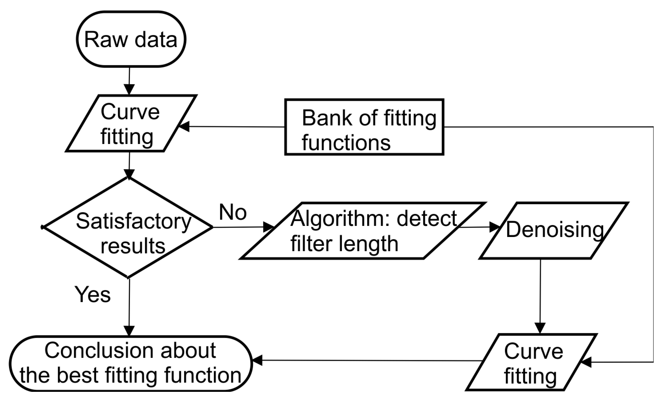
| Algorithm 1 for optimum moving average filter length identification. |
| for kk from 3 to 52 |
| data1_filtered=movemean(data1,kk) |
| data2_filtered=movemean(data2,kk) |
| A = [data1(1:length(min(data1, data2)))’ |
| data2(1:length(min(data1, data2)))’]; |
| % alternatively zero padding can be used that all vectors have the same length. |
| d = (A*A’)/(N − 1); |
| e = d/max(max(d)); |
| zb(k) = sum(sum(dist(e-ones(size(e))))); |
| end; |
| find(zb == min(zb)) |
| where N = length(min(data1, data2)). |
4. Results
4.1. Analysis by Year
4.2. Analysis by Seasons
5. Discussion and Conclusions
- non-uniform time sampling (leading to wrong curve angle between the interpolating points), and
- average (which depends on the route the ship was sailing at the time of data acquisition, and the sailing hours on a specific day).
Author Contributions
Funding
Conflicts of Interest
Appendix A
| Linear fitting (1) | a = 0.01021 (−0.1528, 0.1732), b = 2.519·10−6 (3.792·10−7, 4.658·10−6), c = 28.91 (28.74, 29.08) |
| Exponential of 1st order (2) | a = 29.25 (29.02, 29.48), b = −3.011·10−5 (−6.18·10−5, 1.573·10−6) |
| Exponential of 2nd order (3) | a = 30.39 (30.22, 30.57), b = −0.00035 (−0.0003961, −0.0003039), c = 0.002414 (−0.0005264, 0.005354), d = 0.01832 (0.01554, 0.02109) |
| Fourier 1 (5) | a0 = 6.872·107 (−1.162·1015, 1.162·1015), a1 = −6.872·107 (−1.162·1015, 1.162·1015), b1 = 2.12·104 (−1.792·1011, 1.792·1011), ω = −1.377·10−6 (−11.64, 11.64) |
| Fourier 2 (6) | a0 = 4.758·109 (−2.346·1014, 2.346·1014), a1 = −6.344e+09 (−3.128·1014, 3.127·1014), b1 = −5.466·107 (−2.021·1012, 2.021·1012), a2 = 1.586·109 (−7.818·1013, 7.818·1013), b2 = 2.733·107 (−1.011·1012, 1.011·1012), ω = 4.293·10−5 (−0.529, 0.5291) |
| Fourier 8 (7) | a0 = −8.62·106 (−5.631·107, 3.907·107), a1 = 6.305·106 (−3.368·107, 4.629·107), b1 = 1.433·107 (−6.25·107, 9.116·107), a2 = 7.899·106 (−2.917·107, 4.497·107), b2 = −8.618·106 (−6.156·107, 4.432·107), a3 = −6.728·106 (−4.564·107, 3.218·107), b3 = −2.288·106 (−7.388·106, 2.812·106), a4 = 2.967·105 (−6.255·106, 6.848·106), b4 = 3.439·106 (−1.443·107, 2.131·107), a5 = 1.139·106 (−3.655·106, 5.932·106), b5 = −6.212·105 (−5.908·106, 4.665·106), a6 = −2.82·105 (−2.176·106, 1.612·106), b6 = −2.183·105 (−7.059·105, 2.694·105), a7 = −1.572·104 (−9.789·104, 6.645·104), b7 = 6.237·104 (−2.793·105, 4.041·105), a8 = 5689 (−1.772·104, 2.909·104), b8 = −940.6 (−2.177·104, 1.988·104), ω = 0.00524 (0.003601, 0.006878) |
| Gaussian 1 (9) | a1 = 3.427·1014 (−3.9·1020, 3.9·1020), b1 = −2.005·106 (−7.582·1010, 7.581·1010), c1 = 3.655·105 (−6.909·109, 6.91·109) |
| Gaussian 2 (10) | a1 = 2.511·1013 (−7.073·1016, 7.078·1016), b1 = 5051 (−4.541·105, 4.642·105), c1 = 861.5 (−4.259·104, 4.431·104), a2 = 31.26 (23, 39.52), b2 = −239 (−1875, 1397), c2 = 1316 (−3279, 5910) |
| Gaussian 3 (A2) | a1 = 4.832·1013 (−2.725·1017, 2.726·1017), b1 = 6316 (−1.167·106, 1.18·106), c1 = 1096 (−1.102·105, 1.124·105), a2 = 4.068 (0.9324, 7.204), b2 = 1.883 (−16.1, 19.86), c2 = 43.76 (23.13, 64.38), a3 = 28.29 (9.087, 47.5), b3 = 104 (−323, 531.1), c3 = 473.6 (−422.7, 1370) |
| Gaussian 7 (A3) | a1 = 67.24 (−1483, 1617), b1 = 1033 (−1.778·104, 1.985·104), c1 = 705.8 (−1.017·104, 1.159·104), a2 = 23.55 (−64.26, 111.4), b2 = −9.979 (−35.28, 15.32), c2 = 138.8 (−90.6, 368.3), a3 = 10.09 (−10.02, 30.2), b3 = 171.9 (140.2, 203.6), c3 = 58.59 (9.888, 107.3), a4 = −7.617 (−2314, 2298), b4 = 284.8 (−70.82, 640.5), c4 = 43.15 (−808.4, 894.7), a5 = 2.474 (−0.5536, 5.502), b5 = 100.5 (93.52, 107.4), c5 = 29.94 (17.49, 42.39), a6 = 1.201 (−19.26, 21.66), b6 = 349.6 (252.2, 447), c6 = 30.59 (−61.28, 122.5), a7 = 14.42 (−2241, 2269), b7 = 277.2 (−838.6, 1393), c7 = 48.2 (−165.1, 261.5) |
| Polynomial 1 (11) | p1 = −0.0008497 (−0.001771, 7.112·10−5), p2 = 29.25 (29.01, 29.48) |
| Polynomial 2 (12) | p1 = 6.516·10−5 (5.972·10−5, 7.061·10−5), p2 = −0.0292 (−0.03164, −0.02675), p3 = 31.31 (31.07, 31.54) |
| Polynomial 3 (13) | p1 = 1.807·10−7 (1.343·10−7, 2.272·10−7), p2 = −5.277·10−5 (−8.352·10−5, −2.202·10−5), p3 = −0.008652 (−0.01441, −0.002893), p4 = 30.56 (30.27, 30.85) |
| Power 1 (14) | a = 31.41 (30.8, 32.01), b = −0.01529 (−0.01903, −0.01156) |
| Power 2 (15) | a= 5.338 (4.078, 6.597), b = −0.3466 (−0.5568, −0.1364), c = 28.08 (27.17, 28.98) |
| Rational 1/1 (16) | p1 = 26.56 (25.81, 27.31), p2 = −14.02 (−19.49, −8.555), q1 = −2.457 (−2.51, −2.404) |
| Rational 2/1 (17) | p1 = −0.0007214 (−0.001646, 0.0002029), p2 = 29.21 (28.97, 29.44), p3 = −80.3 (−95.63, −64.96), q1 = −2.77 (−3.257, −2.283) |
| Rational 3/1 (18) | p1 = 6.501·10−5 (5.95·10−5, 7.051·10−5), p2 = −0.02954 (−0.03205, −0.02703), p3 = 31.49 (31.24, 31.73), p4 = −208.4 (−255.8, −161.1), q1 = −6.665 (−8.17, −5.161) |
| Rational 3/2 (19) | p1 = −0.0006458 (−0.001574, 0.0002824), p2 = 29.19 (28.94, 29.43), p3 = −279.9 (−305.2, −254.6), p4 = 645.2 (522.9, 767.4), q1 = −9.623 (−10.42, −8.825), q2 = 22.25 (18.36, 26.14) |
| Rational 5/3 (20) | p1 = 6.325·10−5 (5.593·10−5, 7.057·10−5), p2 = −0.02889 (−0.03347, −0.02431), p3 = 31.51 (30.55, 32.47), p4 = −371.8 (−993.9, 250.3), p5 = 1140 (−5307, 7586), p6 = 184.8 (−1.71·104, 1.747·104), q1 = −11.96 (−31.33, 7.415), q2 = 37.02 (−166.3, 240.4), q3 = 5.183 (−543.4, 553.8) |
| Fitness Function | SSE | R-Square | RMSE | Adjusted R-Square |
|---|---|---|---|---|
| Smoothing spline, p = 0.99876718875 | 0.0003582 | 1 | 0.006983 | 1 |
| p = 0.9 | 0.1907 | 0.9997 | 0.03309 | 0.9993 |
| p = 0.309432 | 0.9227 | 0.9986 | 0.05477 | 0.998 |
| Fourier 8 | 39.79 | 0.9389 | 0.3093 | 0.9364 |
| Gaussian 7 | 44.33 | 0.9319 | 0.3276 | 0.9286 |
| Gaussian 3 | 152.1 | 0.7663 | 0.5983 | 0.7619 |
| Fourier 2 | 159.1 | 0.7556 | 0.6097 | 0.7527 |
| Exponential of 2nd order | 205.2 | 0.6848 | 0.6907 | 0.6826 |
| Gaussian 2 | 217.1 | 0.6665 | 0.7121 | 0.6626 |
| Polynomial 3 | 248.9 | 0.6176 | 0.7608 | 0.6149 |
| Rational 5/3 | 281.3 | 0.5679 | 0.8135 | 0.5598 |
| Rational 3/1 | 282.4 | 0.5661 | 0.8113 | 0.5621 |
| Fourier 1 | 282.7 | 0.5656 | 0.8109 | 0.5626 |
| Polynomial 2 | 282.7 | 0.5656 | 0.8099 | 0.5636 |
| Power 2 | 549.4 | 0.1559 | 1.129 | 0.152 |
| Power 1 | 569.2 | 0.1255 | 1.148 | 0.1235 |
| Rational 3/2 | 634 | 0.02602 | 1.217 | 0.01464 |
| Rational 2/1 | 638.2 | 0.01947 | 1.218 | 0.01263 |
| Linear fitting | 642.9 | 0.01231 | 1.221 | 0.007731 |
| Exponential of 1st order | 645.8 | 0.007776 | 1.223 | 0.005479 |
| Gaussian 1 | 645.8 | 0.007772 | 1.224 | 0.003168 |
| Polynomial 1 | 646 | 0.007557 | 1.223 | 0.00526 |
| Rational 1/1 | 2.66 × 10⁴ | −39.87 * | 7.856 | −40.06 * |
| Fitness Function | Fit-Domain (Samples 1–434) | Prediction Interval (Samples 435–829) | Total Range (Samples 1–829) | Comment |
|---|---|---|---|---|
| Smoothing spline, p = 0.99876718875 | 1 | 1 | 1 | The best fit |
| p = 0.9 | 0.9997 | 0.9987 | 0.9919 | Near the best fit |
| p = 0.309432 | 0.9986 | 0.9955 | 0.9501 | Near the best fit |
| Gaussian 7 | 0.9319 | 0.9599 | 0.6899 | The best fit if smoothing splines are not taken into account |
| Fourier 8 | 0.9389 | 0.934 | 0.7713 | |
| Gaussian 3 | 0.7663 | 0.7583 | 0.5583 | |
| Rational 5/3 | 0.56 | 0.6949 | 0.5008 | |
| Rational 3/2 | 0.5656 | 0.6666 | −3.154 * | Not good for calculations |
| Fourier 2 | 0.7556 | 0.6513 | 0.6933 | |
| Gaussian 2 | 0.6665 | 0.6462 | 0.504 | |
| Polynomial 3 | 0.6176 | 0.6247 | 0.4774 | |
| Fourier 1 | 0.5656 | 0.6236 | 0.5708 | |
| Exponential 2 | 0.6848 | 0.5763 | 0.5848 | |
| Power 2 | 0.1559 | 0.5335 | 0.4715 | |
| Gaussian 1 | 0.007772 | 0.5297 | 0.5667 | |
| Rational 3/1 | 0.5659 | 0.529 | 0.4613 | |
| Rational 2/1 | 0.01768 | 0.5283 | 0.5817 | Too low |
| Polynomial 2 | 0.5656 | 0.5282 | 0.4597 | |
| Polynomial 1 | 0.007557 | 0.5272 | 0.3788 | Too low for column1 |
| Exponential 1 | 0.007776 | 0.5256 | 0.486 | Too low for column1 |
| Linear fitting | 0.01231 | 0.5023 | 0.5635 | Too low for column1 |
| Power 1 | 0.1255 | 0.3073 | 0.1848 | |
| Rational 1/1 | 0.008808 | 0.003205 | 0.1977 | Too low |
| Linear fitting (1) | a = 0.01683 (−0.4147, 0.4484), b = −0.000439 (−0.0005423, −0.0003357), c = 30.13 (29.7, 30.57) |
| Exponential of 1st order (2) | a = 31.25 (30.63, 31.87), b = −0.001501 (−0.001827, −0.001175) |
| Exponential of 2nd order (3) | a = 31.57 (30.81, 32.33), b = −0.00183 (−0.002467, −0.001192), c = 7.661·10−5 (−0.001465, 0.001618), d = 0.09373 (−0.09131, 0.2788) |
| Fourier 1 (5) | a0 = 28.8 (28.6, 29.01), a1 = 0.09534 (−0.4701, 0.6608), b1 = 2.519 (2.217, 2.821), ω = 0.05844 (0.05501, 0.06188) |
| Fourier 2 (6) | a0 = 28.82 (28.67, 28.96), a1 = 0.1301 (−0.1963, 0.4566), b1 = 2.519 (2.301, 2.736), a2 = −1.042 (−1.245, −0.8392), b2 = 0.02157 (−0.2299, 0.273), ω = 0.05837 (0.05573, 0.061) |
| Fourier 8 (7) | a0 = −1.122·1012 (−7.808·1013, 7.584·1013), a1 = 1.699·1012 (−1.173·1014, 1.207·1014), b1 = 1.061·1012 (−6.774·1013, 6.986·1013), a2 = −6.233·1011 (−4.929·1013, 4.805·1013), b2 = −1.278·1012 (−8.583·1013, 8.327·1013), a3 = −8.302·1010 (−1.999·1011, 3.384·1010), b3 = 7.891·1011 (−5.367·1013, 5.525·1013), a4 = 2.104·1011 (−1.157·1013, 1.199·1013), b4 = −2.69·1011 (−2.053·1013, 1.999·1013), a5 = −1.03·1011 (−6.63·1012, 6.424·1012), b5 = 3.73·1010 (−3.696·1012, 3.771·1012), a6 = 2.414·1010 (−1.672·1012, 1.72·1012), b6 = 5.209·109 (−4.283·109, 1.47·1010), a7 = −2.504·109 (−2.098·1011, 2.047·1011), b7 = −2.443·109 (−1.241·1011, 1.192·1011), a8 = 5.484·107 (−7.873·109, 7.982·109), b8 = 2.28·108 (−1.38·1010, 1.426·1010), ω = 0.009698 (−0.03157, 0.05097) |
| Gaussian 1 (9) | a1 = 34.57 (12.13, 57), b1 = −183.4 (−1057, 689.9), c1 = 561.6 (−470.3, 1594) |
| Gaussian 2 (10) | a1 = 26.05 (15.26, 36.83), b1 = 14.46 (8.582, 20.34), c1 = 44.1 (35.12, 53.08), a2 = 27.11 (25.91, 28.31), b2 = 103.9 (98.54, 109.3), c2 = 70.06 (27.97, 112.2) |
| Gaussian 3 (A2) | a1 = 5.155 (4.873, 5.437), b1 = 26.16 (25.76, 26.57), c1 = 9.728 (9.011, 10.44), a2 = −1.671 (−1.947, −1.396), b2 = 72.03 (70.63, 73.44), c2 = 12.67 (9.922, 15.43), a3 = 28.78 (28.59, 28.98), b3 = 14.29 (−15.42, 44), c3 = 410.3 (269.1, 551.6) |
| Gaussian 7 (A3) | a1 = 4.437 (3.671, 5.202), b1 = 26.49 (25.87, 27.11), c1 = 8.597 (7.324, 9.869), a2 = 29.6 (28.86, 30.34), b2 = 22.63 (13.09, 32.18), c2 = 107 (68.95, 145.1), a3 = 0.4699 (−0.03077, 0.9705), b3 = 42.14 (40.67, 43.6), c3 = 1.975 (−0.6027, 4.552), a4 = 1.863 (0.6962, 3.029), b4 = 55.07 (54.4, 55.75), c4 = 3.957 (2.218, 5.697), a5 = 12.85 (−13.58, 39.29), b5 = 119 (62.36, 175.7), c5 = 29.6 (−249.7, 308.9), a6 = 2.819 (−70.61, 76.25), b6 = 85.94 (23.4, 148.5), c6 = 17.51 (−73.16, 108.2), a7 = 0.6927 (−0.2962, 1.682), b7 = 65.57 (63.04, 68.1), c7 = 4.351 (0.2728, 8.43) |
| Polynomial 1 (11) | p1 = −0.04331 (−0.05269, −0.03393), p2 = 31.19 (30.6, 31.78) |
| Polynomial 2 (12) | p1 = −7.924·10−6 (−0.0003428, 0.000327), p2 = −0.04244 (−0.08046, −0.004409), p3 = 31.17 (30.27, 32.08) |
| Polynomial 3 (13) | p1 = 4.488·10−5 (3.633·10−5, 5.342·10−5), p2 = −0.007412 (−0.008842, −0.005983), p3 = 0.2848 (0.217, 0.3527), p4 = 28.11 (27.24, 28.97) |
| Power 1 (14) | a = 32.62 (31.08, 34.16), b = −0.03351 (−0.04599, −0.02103) |
| Power 2 (15) | a = −0.0117 (−0.05463, 0.03122), b = 1.274 (0.5054, 2.042), c = 30.86 (29.9, 31.81) |
| Rational 1/1 (16) | p1 = 28.8 (28.39, 29.2), p2 = −45.01 (−143.4, 53.39), q1 = −1.57 (−4.969, 1.828) |
| Rational 2/1 (17) | p1 = −0.04398 (−0.05356, −0.0344), p2 = 31.59 (30.91, 32.27), p3 = −257.8 (−277.1, −238.4), q1 = −8.275 (−8.957, −7.593) |
| Rational 3/1 (18) | p1 = 4.597e−05 (−0.0002944, 0.0003864), p2 = −0.04994 (−0.08985, −0.01003), p3 = 31.54 (30.5, 32.58), p4 = −91.31 (−111.2, −71.39), q1 = −2.9 (−3.59, −2.21) |
| Rational 3/2 (19) | p1 = −0.04523 (−0.05495, −0.03552), p2 = 31.92 (31.18, 32.66), p3 = −416.9 (−443.9, −390), p4 = 1157 (972.2, 1342), q1 = −13.28 (−14.23, −12.32), q2 = 37.01 (30.4, 43.63) |
| Rational 5/3 (20) | p1 = 0.0004295 (0.0002086, 0.0006504), p2 = −0.08024 (−0.1215, −0.03895), p3 = 31.99 (29.48, 34.49), p4 = −1545 (−1626, −1465), p5 = 2.44·104 (2.175·104, 2.704·104), p6 = −4.617·104 (−6.472·104, −2.762·104), q1 = −52.8 (−55.81, −49.79), q2 = 841.7 (747.9, 935.5), q3 = −1592 (−2210, −973.6) |
| Fitness Function | SSE | R-Square | RMSE | Adjusted R-Square |
|---|---|---|---|---|
| Smoothing spline, p = 0.99876718875 | 0.0008646 | 1 | 0.02183 | 0.9999 |
| Smoothing spline, p = 0.9 | 0.4474 | 0.999 | 0.1018 | 0.9976 |
| p = 0.309432 | 1.994 | 0.9957 | 0.1614 | 0.9939 |
| Gaussian 7 | 5.886 | 0.9872 | 0.2586 | 0.9843 |
| Fourier 8 | 7.823 | 0.983 | 0.2932 | 0.9799 |
| Gaussian 3 | 11.01 | 0.9761 | 0.3319 | 0.9742 |
| Rational 5/3 | 19.51 | 0.9577 | 0.4418 | 0.9543 |
| Fourier 2 | 59.3 | 0.8713 | 0.7588 | 0.8651 |
| Gaussian 2 | 64.52 | 0.86 | 0.7915 | 0.8532 |
| Fourier 1 | 119.1 | 0.7415 | 1.065 | 0.7341 |
| Polynomial 3 | 127.1 | 0.7241 | 1.1 | 0.7163 |
| Rational 3/2 | 245.1 | 0.4683 | 1.542 | 0.4425 |
| Exponential of 2nd order | 246.9 | 0.4642 | 1.533 | 0.4489 |
| Rational 2/1 | 251.7 | 0.4538 | 1.548 | 0.4382 |
| Rational 3/1 | 251.9 | 0.4533 | 1.556 | 0.4323 |
| Power 2 | 254.9 | 0.447 | 1.551 | 0.4365 |
| Gaussian 1 | 258 | 0.4402 | 1.56 | 0.4297 |
| Polynomial 1 | 258.5 | 0.4392 | 1.554 | 0.4339 |
| Polynomial 2 | 258.5 | 0.4392 | 1.561 | 0.4286 |
| Exponential of 1st order | 258.7 | 0.4387 | 1.555 | 0.4334 |
| Linear fitting | 275.9 | 0.4014 | 1.613 | 0.3901 |
| Power 1 | 363.9 | 0.2103 | 1.844 | 0.2029 |
| Rational 1/1 | 460.4 | 0.0009077 | 2.084 | −0.01794 |
| Fitness Function | Fit-Domain (Summers 1 and 2) | Prediction Interval (Summers 3 and 4) | Total Range (all 4 Summers) | Comment |
|---|---|---|---|---|
| Smoothing spline p = 0.9987671 | 1 | 1 | 0.9995 | The best fit |
| Smoothing spline p = 0.9 | 0.999 | 0.9978 | 0.996 | Near best fit |
| Gaussian 7 | 0.9872 | 0.9931 | 0.9267 | Best results when smoothing splines are excluded |
| Smoothing spline p = 0.3094 | 0.9957 | 0.9922 | 0.9858 | Near best fit |
| Fourier 8 | 0.983 | 0.9873 | 0.9442 | Best results when smoothing splines are excluded |
| Gaussian 3 | 0.9761 | 0.9555 | 0.8218 | |
| Fourier 2 | 0.8713 | 0.9418 | 0.8169 | |
| Exponential of 2nd order | 0.4642 | 0.8828 | 0.5431 | |
| Gaussian 2 | 0.86 | 0.8828 | 0.7003 | |
| Rational 2/1 | 0.4516 | 0.8823 | 0.5421 | |
| Polynomial 3 | 0.7241 | 0.8804 | 0.5431 | |
| Rational 5/3 | 0.7961 | 0.8794 | −4.337 ** | |
| Rational 3/1 | 0.4539 | 0.8785 | 0.5471 | |
| Fourier 1 | 0.7415 | 0.8784 | 0.5373 | |
| Polynomial 2 | 0.4392 | 0.8784 | 0.5431 | |
| Rational 1/1 | 0.0009076 | 0.8244 | 0.004622 | |
| Power 1 | 0.2103 | 0.7884 | 0.3223 | |
| Power 2 | 0.447 | 0.7884 | 0.5442 | |
| Exponential of 1st order | 0.4387 | 0.5604 | 0.5334 | |
| Rational 3/2 | 0.5441 | 0.5583 | 0.5466 | |
| Polynomial 1 | 0.4392 | 0.5289 | 0.5376 | |
| Linear fitting | 0.4014 | 0.2454 | 0.5263 | |
| Gaussian 1 | 0.4402 | N/A * | 0.543 |
| Linear fitting (1) | a = −0.04539 (−0.3596, 0.2688), b = 0.0002863 (0.000223, 0.0003495), c = 28.74 (28.42, 29.06) |
| Exponential of 1st order (2) | a = 28.59 (28.07, 29.1), b = 0.0006785 (0.0004205, 0.0009364) |
| Exponential of 2nd order (3) | a = 20.28 (13.76, 26.8), b = −0.01133 (−0.01737, −0.005289), c = 11.39 (4.565, 18.22), and d = 0.007709 (0.004173, 0.01125) |
| Fourier 1 (5) | a0 = 30.23 (29.9, 30.56), a1 = 1.47 (1.117, 1.824), b1 = −1.839 (−2.402, −1.276), ω = 0.04373 (0.03873, 0.04873) |
| Fourier 2 (6) | a0 = 30.1 (29.93, 30.27), a1 = 1.146 (0.4727, 1.819), b1 = −1.75 (−2.099, −1.401), a2 = −0.4874 (−0.729, −0.2458), b2 = 0.3735 (−0.194, 0.9409), ω = 0.04314 (0.03784, 0.04844) |
| Fourier 8 (7) | a0 = 29.82 (29.8, 29.84), a1 = 1.851 (1.794, 1.907), b1 = −0.9324 (−1.015, −0.8492), a2 = −0.3776 (−0.4395, −0.3156), b2 = −0.3376 (−0.3814, −0.2937), a3 = 0.1491 (0.07512, 0.2231), b3 = −0.4124 (−0.4374, −0.3874), a4 = −0.04963 (−0.1024, 0.003145), b4 = −0.07979 (−0.1323, −0.02726), a5 = −0.2298 (−0.2614, −0.1982), b5 = 0.1685 (0.101, 0.236), a6 = −0.01184 (−0.06022, 0.03655), b6 = −0.1228 (−0.1505, −0.09501), a7 = −0.1947 (−0.2209, −0.1685), b7 = −0.005933 (−0.09148, 0.07961), a8 = −0.07079 (−0.1274, −0.0142), b8 = 0.09574 (0.05283, 0.1386), ω = 0.05152 (0.05085, 0.05219) |
| Gaussian 1 (9) | a1 = 4.026·1096 (−1.429·10103, 1.429·10103), b1 = 6.461·105 (−1.047·1010, 1.047·1010), c1 = 4.365·104 (−3.536·108, 3.536·108) |
| Gaussian 2 (10) | a1 = 25.59 (17.38, 33.79), b1 = 123.3 (120.4, 126.3), c1 = 55.5 (43.33, 67.67), a2 = 30.31 (29.55, 31.07), b2 = 1.598 (−2.844, 6.039), c2 = 95.27 (56.39, 134.1) |
| Gaussian 3 (A2) | a1 = 32.85 (32.26, 33.43), b1 = 130 (116.7, 143.3), c1 = 155 (126, 184), a2 = 12.88 (10.6, 15.15), b2 = −1.083 (−3.304, 1.138), c2 = 17.47 (11.68, 23.26), a3 = 7.65 (4.925, 10.38), b3 = 27.5 (21.28, 33.73), c3 = 20.62 (15.55, 25.69) |
| Gaussian 7 (A3) | a1 = 32.69 (30.32, 35.06), b1 = 112.7 (108.1, 117.4), c1 = 27.42 (18.18, 36.67), a2 = 30.76 (29.99, 31.53), b2 = 3.096 (−2.256, 8.448), c2 = 45.15 (8.354, 81.94), a3 = 10.8 (−35.29, 56.89), b3 = 82.33 (80.03, 84.63), c3 = 11.69 (2.008, 21.37), a4 = 1.048 (−92.15, 94.25), b4 = 26.08 (−82.89, 135.1), c4 = 11.07 (−89.58, 111.7), a5 = 20.26 (−1.597, 42.11), b5 = 63.03 (56, 70.06), c5 = 20.46 (−48.7, 89.62), a6 = 7.41 (−95.68, 110.5), b6 = 37.05 (−22.28, 96.38), c6 = 14.19 (−81.59, 110), a7 = 4.07 (1.256, 6.884), b7 = 95.85 (94.26, 97.43), c7 = 7.985 (6.273, 9.697) |
| Polynomial 1 (11) | p1 = 0.01943 (0.01172, 0.02714), p2 = 28.62 (28.09, 29.15) |
| Polynomial 2 (12) | p1 = 0.001234 (0.001121, 0.001347), p2 = −0.1274 (−0.1412, −0.1136), p3 = 31.56 (31.2, 31.91) |
| Polynomial 3 (13) | p1 = −1.947·10−6 (−5.712·10−6, 1.818·10−6), p2 = 0.001581 (0.0009001, 0.002263), p3 = −0.144 (−0.179, −0.109), p4 = 31.72 (31.24, 32.21) |
| Power 1 (14) | a = 29.11 (27.92, 30.3), b = 0.005937 (−0.004536, 0.01641) |
| Power 2 (15) | a = 1.284·10−10 (−9.654·10−10, 1.222·10−10), b = 5.096 (3.291, 6.901), c = 28.99 (28.72, 29.27) |
| Rational 1/1 (16) | p1 = 29.69 (29.3, 30.08), p2 = 17.66 (−236.1, 271.4), q1 = 0.5237 (−7.731, 8.778) |
| Rational 2/1 (17) | p1 = 1.366 (−3.127, 5.859), p2 = −110.5 (−574.6, 353.7), p3 = 3.269·104 (−8.198·104, 1.474·105), q1 = 1033 (−2601, 4666) |
| Rational 3/1 (18) | p1 = 0.001356 (0.001122, 0.001589), p2 = −0.142 (−0.166, −0.1181), p3 = 31.82 (30.7, 32.94), p4 = 111.7 (−392.1, 615.4), q1 = 3.678 (−12.62, 19.98) |
| Rational 3/2 (19) | p1 = 0.01698 (0.004851, 0.02911), p2 = 29.55 (27.51, 31.58), p3 = −3671 (95% confidence bounds: −4079, −3263), p4 = 1.327·105 (1.116·105, 1.539·105), q1 = −118.8 (−129.5, −108.1), q2 = 4350 (3678, 5021) |
| Rational 5/3 (20) | p1 = 0.00135 (0.001112, 0.001588), p2 = −0.1589 (−0.1877, −0.1301), p3 = 33.7 (31.57, 35.84), p4 = −317.1 (−1029, 394.7), p5 = 38.35 (−6943, 7020), p6 = 3728 (−1.678e+04, 2.424e+04), q1 = −9.637 (−32.02, 12.74), q2 = −0.6917 (−224.9, 223.5), q3 = 123 (−541, 786.9) |
| Fitness Function | SSE | R-Square | RMSE | Adjusted R-Square |
|---|---|---|---|---|
| Smoothing spline, p = 0.99876718875 | 0.0001338 | 1 | 0.008246 | 1 |
| p = 0.9 | 0.07389 | 0.9997 | 0.03972 | 0.9994 |
| p = 0.309432 | 0.4007 | 0.9986 | 0.0695 | 0.9981 |
| Fourier 8 | 0.9464 | 0.9968 | 0.09728 | 0.9962 |
| Gaussian 7 | 0.9249 | 0.9968 | 0.09765 | 0.9962 |
| Gaussian 3 | 9.53 | 0.9674 | 0.2957 | 0.965 |
| Rational 3/2 | 14.8 | 0.9494 | 0.3635 | 0.9471 |
| Fourier 2 | 17.1 | 0.9415 | 0.3907 | 0.9389 |
| Gaussian 2 | 19.35 | 0.9338 | 0.4157 | 0.9308 |
| Fourier 1 | 32.92 | 0.8874 | 0.5374 | 0.8844 |
| Rational 5/3 | 45.34 | 0.8449 | 0.6449 | 0.8335 |
| Rational 3/1 | 45.43 | 0.8446 | 0.6341 | 0.8391 |
| Polynomial 3 | 46.8 | 0.8399 | 0.6407 | 0.8357 |
| Rational 2/1 | 46.98 | 0.8393 | 0.6419 | 0.8351 |
| Polynomial 2 | 47.23 | 0.8384 | 0.6409 | 0.8356 |
| Exponential of 2nd order | 47.87 | 0.8362 | 0.648 | 0.8319 |
| Power 2 | 126.3 | 0.5678 | 1.048 | 0.5603 |
| Linear fitting | 172.1 | 0.4114 | 1.223 | 0.4011 |
| Exponential of 1st order | 238.6 | 0.1838 | 1.434 | 0.1767 |
| Gaussian 1 | 238.6 | 0.1838 | 1.44 | 0.1696 |
| Polynomial 1 | 240.7 | 0.1767 | 1.44 | 0.1696 |
| Rational 1/1 | 289.1 | 0.01099 | 1.586 | −0.00621 |
| Power 1 | 289.3 | 0.01042 | 1.579 | 0.001884 |
| Fitness Function | Fit-Domain (Autumns 1 and 2) | Prediction Interval (Autumns 3 and 4) | Total Range (all 4 Autumns) | Comment |
|---|---|---|---|---|
| Smoothing spline, p = 0.99876718875 | 1 | 1 | 1 | The best fit |
| p = 0.9 | 0.9997 | 0.9971 | 0.9984 | |
| p = 0.309432 | 0.9986 | 0.9897 | 0.9942 | |
| Gaussian 7 | 0.9968 | 0.9859 | 0.9742 | Best choice when smoothing splices are excluded. |
| Rational 3/2 | 0.9494 | 0.9741 | 0.6388 | |
| Fourier 8 | 0.9968 | 0.9733 | 0.9494 | Near best choice when smoothing splices are excluded. |
| Gaussian 3 | 0.9674 | 0.9484 | 0.8847 | |
| Rational 5/3 | 0.8449 | 0.8914 | 0.6214 | |
| Fourier 2 | 0.9415 | 0.8814 | 0.791 | |
| Gaussian 2 | 0.9338 | 0.8795 | 0.7352 | |
| Fourier 1 | 0.8874 | 0.8713 | 0.6388 | |
| Polynomial 3 | 0.8399 | 0.865 | 0.6507 | |
| Exponential of 2nd order | 0.8362 | 0.8287 | −4.861 * | * Matlab warning |
| Power 2 | 0.5678 | 0.7995 | 0.6424 | |
| Gaussian 1 | 0.1838 | 0.7959 | 0.6381 | |
| Rational 3/1 | 0.8446 | 0.7953 | 0.6968 | |
| Polynomial 2 | 0.8384 | 0.7931 | 0.6388 | |
| Rational 2/1 | 0.8393 | 0.7909 | 0.4735 | |
| Polynomial 1 | 0.1767 | 0.7858 | 0.473 | |
| Exponential of 1st order | 0.1838 | 0.7812 | 0.4593 | |
| Linear fitting | 0.4114 | 0.7609 | 0.5964 | |
| Power 1 | 0.01042 | 0.4893 | 0.2602 | |
| Rational 1/1 | 0.01099 | 0.02938 | 0.4729 |
| Linear fitting (1) | a = −0.02188 (−0.2189, 0.1752), b = 6.907·10−5 (1.449·10−5, 0.0001237), c = 28.12 (27.92, 28.32) |
| Exponential of 1st order (2) | a = 28.31 (bounds: 28.02, 28.6), and b = −6.32·10−6 (−0.0001787, 0.0001661) |
| Exponential of 2nd order (3) | a = 28.79 (27.71, 29.87), b = −0.00243 (−0.003808, −0.001053), c = 0.6529 (−0.5924, 1.898), d = 0.02388 (0.01006, 0.0377) |
| Fourier 1 (5) | a0 = 28.16 (28.09, 28.23), a1 = 0.5406 (0.3579, 0.7233), b1 = 0.7318 (0.5792, 0.8843), ω = 0.07365 (0.06925, 0.07804) |
| Fourier 2 (6) | a0 = 28.44 (28.31, 28.56), a1 = 0.8091 (0.4632, 1.155), b1 = −0.3872 (−0.8644, 0.09007), a2 = −0.3317 (−0.4104, −0.2531), b2 = 0.1166 (−0.3926, 0.6258), ω = 0.05057 (0.04012, 0.06102) |
| Fourier 8 (7) | a0 = 28.4 (28.31, 28.49), a1 = 0.9113 (0.755, 1.068), b1 = −0.2112 (−0.4711, 0.04881), a2 = −0.2993 (−0.4587, −0.1399), b2 = −0.06535 (−0.2176, 0.08691), a3 = −0.04238 (−0.1884, 0.1037), b3 = −0.1498 (−0.2659, −0.03362), a4 = 0.09473 (−0.03816, 0.2276), b4 = −0.01995 (−0.1303, 0.09044), a5 = −0.1726 (−0.2623, −0.0828), b5 = 0.1299 (−0.1434, 0.4033), a6 = −0.02845 (−0.09781, 0.04091), b6 = 0.0155 (−0.07253, 0.1035), a7 = 0.07436 (−0.0176, 0.1663), b7 = −0.004225 (−0.09292, 0.08447), a8 = −0.06261 (−0.2146, 0.08941), b8 = 0.1033 (−0.0578, 0.2644), ω = 0.05442 (0.05006, 0.05879) |
| Gaussian 1 (9) | a1 = 28.35 (−60.17, 116.9), b1 = −637.7 (−1.061·106, 1.06·106), c1 = 1.529·104 (−1.175·107, 1.178·107) |
| Gaussian 2 (10) | a1 = 19.57 (7.279, 31.86), b1 = 116.5 (110.4, 122.6), c1 = 51.55 (32.7, 70.41), a2 = 28.71 (27.94, 29.48), b2 = 7.058 (0.8335, 13.28), c2 = 97.94 (51.13, 144.8) |
| Gaussian 3 (A2) | a1 = 29.18 (26.94, 31.43), b1 = 113 (106.9, 119.2), c1 = 102.8 (15.34, 190.2), a2 = 21.12 (3.491, 38.75), b2 = −13.39 (−19.73, −7.037), c2 = 61.1 (34.01, 88.18), a3 = 1.117 (0.893, 1.34), b3 = 31.73 (30.94, 32.53), c3 = 5.535 (4.146, 6.924) |
| Gaussian 7 (A3) | a1 = 29.83 (28.1, 31.57), b1 = 117.1 (64.29, 170), c1 = 140.8 (−85.14, 366.8), a2 = 14.57 (−13.05, 42.2), b2 = −9.303 (−34.14, 15.53), c2 = 44.71 (−6.636, 96.06), a3 = 1.096 (0.7929, 1.4), b3 = 34.79 (34.52, 35.07), c3 = 1.847 (1.272, 2.422), a4 = 0.5781 (−0.6638, 1.82), b4 = 46.14 (42.81, 49.47), c4 = 6.095 (0.2361, 11.95), a5 = 1.61 (−0.7591, 3.98), b5 = 29.99 (26.84, 33.14), c5 = 9.895 (3.158, 16.63), a6 = 0.8952 (−1.199, 2.99), b6 = 56.75 (46.22, 67.27), c6 = 11.02 (−5.995, 28.03), a7 = 0.6716 (0.3439, 0.9993), b7 = 79 (78.26, 79.75), c7 = 4.245 (2.401, 6.089) |
| Polynomial 1 (11) | p1 = −0.0001754 (−0.005053, 0.004702), p2 = 28.31 (28.02, 28.6) |
| Polynomial 2 (12) | p1 = 0.0007765 (0.0006731, 0.0008799), p2 = −0.08015 (−0.09115, −0.06916), p3 = 29.69 (29.45, 29.94) |
| Polynomial 3 (13) | p1 = 8.683e−06 (5.058e−06, 1.231e−05), p2 = −0.000565 (−0.001133, 2.833e−06), p3 = −0.02461 (−0.04985, 0.0006242), p4 = 29.2 (28.9, 29.51) |
| Power 1 (14) | a = 28.99 (28.41, 29.57), b = −0.006629 (−0.01191, −0.001349) |
| Power 2 (15) | a = 1.526 (bounds: 0.4475, 2.604), b = −0.4284 (−1.337, 0.4801), and c = 27.95 (26.86, 29.03) |
| Rational 1/1 (16) | p1 = 28.28 (28.14, 28.43), p2 = −50.27 (−80.95, −19.59), q1 = −1.783 (−2.842, −0.7249) |
| Rational 2/1 (17) | p1 = 0.0004235 (bounds: −0.00459, 0.005437), p2 = 28.26 (27.95, 28.57), p3 = −50.2 (−80.05, −20.35), q1 = −1.782 (−2.812, −0.7532) |
| Rational 3/1 (18) | p1 = 0.001457 (0.0008546, 0.002059), p2 = −0.1586 (−0.2211, −0.09621), p3 = 31.29 (30.13, 32.46), p4 = 735.3 (−433.5, 1904), q1 = 25.65 (−14.72, 66.02) |
| Rational 3/2 (19) | p1 = 0.0005795 (−0.004503, 0.005662), p2 = 28.25 (27.88, 28.61), p3 = −338.4 (−388.7, −288.1), p4 = 894 (bounds: 596.2, 1192), q1 = −11.98 (−13.69, −10.27), q2 = 31.66 (21.45, 41.86) |
| Rational 5/3 (20) | p1 = 0.001389 (0.0009086, 0.001869), p2 = −0.1762 (−0.2345, −0.1179), p3 = 34.02 (32.02, 36.01), p4 = −70.51 (−935, 793.9), p5 = −2716 (−1.161·104, 6177), p6 = 1.366·104 (bounds: −1.202·104, 3.934·104), q1 = −0.4298 (−30.31, 29.45), q2 = −103.4 (−412.6, 205.8), q3 = 487.4 (−412.4, 1387) |
| Fitness Function | SSE | R-Square | RMSE | Adjusted R-Square |
|---|---|---|---|---|
| Smoothing spline, p = 0.99876718875 | 0.0005719 | 1 | 0.01837 | 0.9994 |
| p = 0.9 | 0.2665 | 0.995 | 0.08124 | 0.9875 |
| p = 0.309432 | 0.9664 | 0.9819 | 0.1162 | 0.9745 |
| Gaussian 7 | 1.102 | 0.9794 | 0.1167 | 0.9743 |
| Fourier 8 | 1.997 | 0.9626 | 0.1542 | 0.9551 |
| Fourier 2 | 7.085 | 0.8675 | 0.2717 | 0.8605 |
| Gaussian 2 | 8.046 | 0.8495 | 0.2895 | 0.8416 |
| Fourier 1 | 8.601 | 0.8391 | 0.2962 | 0.8342 |
| Rational 5/3 | 11.54 | 0.7841 | 0.3523 | 0.7655 |
| Rational 3/1 | 11.6 | 0.7831 | 0.3457 | 0.7741 |
| Polynomial 3 | 13.4 | 0.7494 | 0.3697 | 0.7417 |
| Exponential of 2nd order | 14.6 | 0.7268 | 0.386 | 0.7184 |
| Polynomial 2 | 16.49 | 0.6916 | 0.4081 | 0.6853 |
| Linear fitting | 50.23 | 0.06032 | 0.7123 | 0.04134 |
| Power 1 | 50.38 | 0.05741 | 0.7098 | 0.04798 |
| Rational 3/2 | 52.47 | 0.01834 | 0.7393 | −0.03279 * |
| Rational 2/1 | 52.78 | 0.01254 | 0.7339 | −0.01768 * |
| Rational 1/1 | 52.8 | 0.01226 | 0.7303 | −0.007692 * |
| Gaussian 3 | 3.794 | 0.929 | 0.202 | 0.9229 |
| Power 2 | 49.4 | 0.0758 | 0.7064 | 0.05713 |
| Exponential of 1st order | 53.45 | 5.189·10−5 | 0.7311 | −0.009948 * |
| Polynomial 1 | 53.45 | 5.09·10−5 | 0.7311 | −0.009949 * |
| Gaussian 1 | 53.46 | −0.0001639 * | 0.7348 | −0.02037 * |
| Fitness Function | Fit-Domain (Winters 1–2) | Prediction Interval (Winters 3–4) | Total Range (all 4 Winters) | Comment |
|---|---|---|---|---|
| Smoothing spline, p = 0.99876718875 | 1 | 1 | 1 | The best fit |
| p = 0.9 | 0.995 | 0.9978 | 0.9985 | |
| Gaussian 7 | 0.9794 | 0.9931 | 0.9267 | |
| Smoothing spline p = 0.309432 | 0.9819 | 0.9922 | 0.9945 | |
| Fourier 8 | 0.9626 | 0.9873 | 0.9761 | |
| Gaussian 3 | 0.929 | 0.9555 | 0.9466 | |
| Fourier 2 | 0.8675 | 0.9418 | 0.9354 | |
| Rational 5/3 | 0.7841 | 0.8829 | 0.9429 | |
| Exponential of 2nd order | 0.7268 | 0.8828 | 0.8571 | |
| Gaussian 2 | 0.8495 | 0.8828 | 0.9104 | |
| Polynomial 3 | 0.7494 | 0.8804 | 0.8665 | |
| Fourier 1 | 0.8391 | 0.8784 | 0.8458 | |
| Polynomial 2 | 0.6916 | 0.8784 | 0.8458 | |
| Rational 3/1 | 0.7831 | 0.881 | 0.8477 | |
| Power 1 | 0.05741 | 0.7884 | 0.3671 | |
| Power 2 | 0.0758 | 0.7884 | 0.8614 | |
| Exponential of 1st order | 5.189·10−5 | 0.5604 | 0.656 | |
| Rational 3/2 | 0.01834 | 0.5397 | 0.9403 | |
| Rational 2/1 | 0.01254 | 0.5332 | 0.6771 | |
| Polynomial 1 | 5.09·10−5 | 0.5289 | 0.6745 | |
| Linear fitting | 0.06032 | 0.2454 | 0.816 | |
| Rational 1/1 | 0.01226 | 0.01329 | 0.0109 | |
| Gaussian 1 | −0.0001639 * | N/A | 0.841 | Inf computed by model function, fitting cannot continue. |
| Linear fitting (1) | a = −0.001745 (−0.1453, 0.1418), b = −2.716·10−5 (−6.444·10−5, 1.011·10−5), c = 29.09 (28.94, 29.23) |
| Exponential of 1st order (2) | a = 28.97 (28.77, 29.18), b = 2.768·10−5 (−8.86·10−5, 0.000144) |
| Exponential of 2nd order (3) | a = −0.01843 (−0.07621, 0.03936), b = 0.04838 (0.02118, 0.07558), c = 28.47 (28.28, 28.65), d = 0.0007368 (0.0003567, 0.001117) |
| Fourier 1 (5) | a0 = 29.09 (29.02, 29.16), a1 = 0.02635 (−0.1644, 0.2171), b1 = −0.5724 (−0.6691, −0.4757), ω = 0.07486 (0.06923, 0.08049) |
| Fourier 2 (6) | a0 = 29.12 (29.06, 29.17), a1 = 0.0604 (−0.05226, 0.1731), b1 = −0.5426 (−0.6154, −0.4699), a2 = −0.1226 (−0.2415, −0.003689), b2 = −0.3169 (−0.4064, −0.2273), ω= 0.07436 (0.07171, 0.077) |
| Fourier 8 (7) | a0 = 28.99 (28.94, 29.04), a1 = −0.502 (−0.5794, −0.4245), b1 = −0.1689 (−0.3016, −0.03619), a2 = −0.0574 (−0.2131, 0.09831), b2 = 0.3611 (0.3103, 0.412), a3 = 0.199 0.1409, 0.2571), b3 = −0.03921 (−0.1616, 0.08319), a4 = −0.03603 (−0.08402, 0.01196), b4 = 0.09401 (0.05168, 0.1363), a5 = 0.08342 (−0.07823, 0.2451), b5 = −0.1118 (−0.17, −0.05353), a6 = −0.1135 (−0.2218, −0.005219), b6 = 0.1204 (−0.04748, 0.2884), a7 = 0.06244 (0.02226, 0.1026), b7 = −0.004121 (−0.08272, 0.07448), a8 = −0.01616 (−0.09508, 0.06275), b8 = 0.07005 (0.02402, 0.1161), ω = 0.05696 (0.05373, 0.06018) |
| Gaussian 1 (9) | a1 = 29.38 (29.26, 29.5), b1 = 54.13 (50.75, 57.51), c1 = 270 (236.6, 303.5) |
| Gaussian 2 (10) | a1 = 29.57 (29.36, 29.77), b1 = 68.9 (59.9, 77.91), c1 = 144.9 (107.5, 182.2), a2 = 6.047 (−1.507, 13.6), b2 = −15.25 (−45.87, 15.36), c2 = 36.4 (8.628, 64.18) |
| Gaussian 3 (A2) | a1 = 1.419 (0.35, 2.487), b1 = 70.92 (66.05, 75.8), c1 = 14.86 (9.047, 20.67), a2 = 78.21 (−4.145·105, 4.147·105), b2 = 6155 (−3.252·107, 3.253·107), c2 = 6144 (−1.623·107, 1.625·107), a3 = −1.338 (−44.12, 41.44), b3 = 101.9 (−435.5, 639.2), c3 = 41.61 (−449.4, 532.6) |
| Gaussian 7 (A3) | a1 = 1.073 (0.8171, 1.329), b1 = 60.96 (60.51, 61.42), c1 = 3.182 (2.307, 4.057), a2 = 29.82 (29.74, 29.9), b2 = 71.53 (70.08, 72.99), c2 = 79.17 (66.86, 91.48), a3 = 1.615 (−19.11, 22.34), b3 = 43.72 (27.25, 60.19), c3 = 7.56 (−7.447, 22.57), a4 = 15.4 (−58.75, 89.55), b4 = −4.202 (−90.21, 81.8), c4 = 18.05 (−271.1, 307.2), a5 = 6.021 (−266.5, 278.5), b5 = 18.45 (−40.3, 77.2), c5 = 13.43 (−288.4, 315.2), a6 = 3.458 (1.835, 5.081), b6 = 107.5 (103.7, 111.3), c6 = 10.99 (7.16, 14.81), a7 = 3.096 (−142.1, 148.3), b7 = 32.69 (−91.44, 156.8), c7 = 10.67 (−113.4, 134.8) |
| Polynomial 1 (11) | p1 = 0.0008112 (−0.002563, 0.004185), p2 = 28.97 (28.77, 29.18) |
| Polynomial 2 (12) | p1 = −0.0003957 (−0.0004937, −0.0002976), p2 = 0.04275 (0.03203, 0.05348), p3 = 28.22 (27.98, 28.47) |
| Polynomial 3 (13) | p1 = −1.111·10−5 (−1.41·10−5, −8.131·10−6), p2 = 0.001371 (0.0008905, 0.001852), p3 = −0.03252 (−0.05451, −0.01053), p4 = 28.9 (28.63, 29.17) |
| Power 1 (14) | a = 28.65 (28.23, 29.06), b = 0.003467 (−0.0003017, 0.007236) |
| Power 2 (15) | a = −0.8686 (−3.288, 1.551), b = −0.2256 (−1.632, 1.181), c = 29.4 (26.49, 32.32) |
| Rational 1/1 (16) | p1 = 29.02 (confidence bounds: 28.91, 29.12), p2 = −50.97 (−125.8, 23.84), q1 = −1.755 (−4.35, 0.8403) |
| Rational 2/1 (17) | p1 = 0.0006562 (confidence bounds: −0.002789, 0.004101), p2 = 28.98 (28.74, 29.22), p3 = −257 (−303.3, −210.7), q1 = −8.865 (−10.48, −7.253) |
| Rational 3/1 (18) | p1 = −0.000405 (−0.0005055, −0.0003045), p2 = 0.0456 (0.03414, 0.05707), p3 = 28.01 (27.72, 28.31), p4 = −116.4 (−147.3, −85.38), q1 = −4.125 (−5.196, −3.054) |
| Rational 3/2 (19) | p1 = −18.77 (−8290, 8252), p2 = 2122 (−9.201·105, 9.244·105), p3 = 1.299·106 (−5.72·108, 5.746·108), p4 = −3.706·106 (−1.638·109, 1.631·109), q1 = 4.631·104 (−2.038·107, 2.048·107), q2 = −1.316·105 (−5.817·107, 5.791·107) |
| Rational 5/3 (20) | p1 = −8.931·10−5 (−0.0003049, 0.0001263), p2 = 0.01715 (−0.03251, 0.0668), p3 = 27.42 (23.49, 31.35), p4 = −4117 (−4561, −3673), p5 = 1.603e+05 (1.304·105, 1.902·105), p6 = −2.4·105 (−4.535·105, −2.649·104), q1 = −145 (bounds: −158.3, −131.6), q2 = 5597 (4569, 6624), q3 = −8388 (−1.586·104, −918.6) |
| Fitness Function | SSE | R-Square | RMSE | Adjusted R-Square |
|---|---|---|---|---|
| Smoothing spline, p = 0.99876718875 | 0.0005042 | 1 | 0.01699 | 0.999 |
| p = 0.9 | 0.2488 | 0.9914 | 0.07735 | 0.9784 |
| p = 0.309432 | 0.8244 | 0.9714 | 0.1058 | 0.9596 |
| Gaussian 7 | 1.407 | 0.9512 | 0.1294 | 0.9395 |
| Fourier 8 | 1.705 | 0.9408 | 0.14 | 0.9293 |
| Gaussian 3 | 5.626 | 0.8047 | 0.2421 | 0.7885 |
| Rational 5/3 | 6.391 | 0.7782 | 0.258 | 0.7598 |
| Fourier 2 | 6.445 | 0.7763 | 0.2552 | 0.765 |
| Gaussian 2 | 10.64 | 0.6307 | 0.3278 | 0.6121 |
| Polynomial 3 | 11.46 | 0.6023 | 0.3368 | 0.5905 |
| Fourier 1 | 12.16 | 0.5781 | 0.347 | 0.5655 |
| Exponential of 2nd order | 13.64 | 0.5265 | 0.3675 | 0.5125 |
| Rational 3/1 | 17.45 | 0.3945 | 0.4177 | 0.3703 |
| Rational 3/2 | 17.48 | 0.3933 | 0.4202 | 0.3627 |
| Gaussian 1 | 17.63 | 0.3882 | 0.4157 | 0.3762 |
| Polynomial 2 | 17.66 | 0.3872 | 0.4161 | 0.3752 |
| Power 2 | 27.83 | 0.03406 | 0.5224 | 0.01512 |
| Power 1 | 27.91 | 0.03153 | 0.5205 | 0.02213 |
| Linear fitting | 28.24 | 0.0201 | 0.5261 | 0.0008901 |
| Rational 2/1 | 28.62 | 0.006746 | 0.5323 | −0.02276 |
| Polynomial 1 | 28.75 | 0.002203 | 0.5284 | −0.007485 |
| Exponential of 1st order | 28.75 | 0.002181 | 0.5284 | −0.007507 * |
| Rational 1/1 | 28.76 | 0.001936 | 0.531 | −0.01763 |
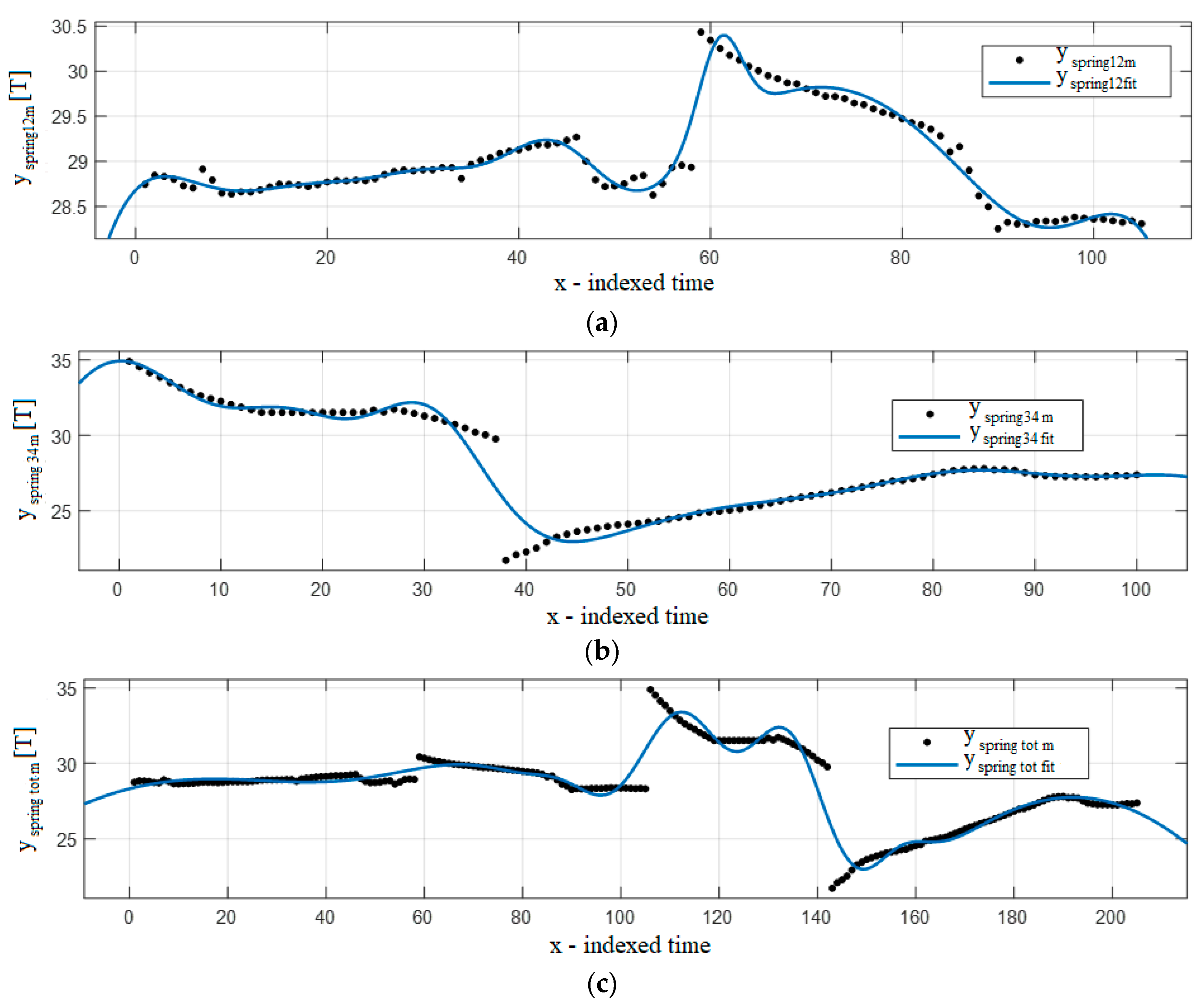
| Fitness Function | Fit-Domain (Springs 1–2) | Prediction Interval (Springs 3–4) | Total Range (all 4 Springs) | Comment |
|---|---|---|---|---|
| Smoothing spline, p = 0.99876718875 | 1 | 1 | 1 | The best fit |
| p = 0.9 | 0.9914 | 0.995 | 0.9918 | |
| p = 0.309432 | 0.9714 | 0.9827 | 0.9717 | |
| Fourier 8 | 0.9408 | 0.9596 | 0.8896 | The best for spring 3–4 when smoothing splines are excluded |
| Gaussian 7 | 0.9512 | 0.9501 | 0.9062 | The best for whole dataset and springs 1–2 when smoothing splines are excluded |
| Gaussian 3 | 0.8047 | 0.9345 | 0.5874 | |
| Rational 3/2 | 0.3933 | 0.9174 | 0.8254 | |
| Fourier 2 | 0.7763 | 0.8365 | 0.5747 | |
| Gaussian 2 | 0.6307 | 0.8252 | 0.5659 | |
| Fourier 1 | 0.5781 | 0.7325 | 0.3169 | |
| Rational 5/3 | 0.7782 | 0.7256 | −66.28 * | |
| Rational 3/1 | 0.3945 | 0.7185 | 0.2409 | |
| Polynomial 3 | 0.6023 | 0.7102 | 0.2664 | |
| Polynomial 2 | 0.3872 | 0.71 | 0.2399 | |
| Exponential of 2nd order | 0.5265 | 0.706 | 0.2258 | |
| Power 2 | 0.03406 | 0.5215 | 0.2072 | |
| Power 1 | 0.03153 | 0.5181 | 0.04345 | |
| Exponential of 1st order | 0.002181 | 0.3752 | 0.1342 | |
| Gaussian 1 | 0.3882 | 0.3752 | 0.2458 | |
| Rational 2/1 | 0.006746 | 0.3558 | 0.1383 | |
| Polynomial 1 | 0.002203 | 0.3518 | 0.1375 | |
| Linear fitting | 0.0201 | 0.1475 | 0.1975 | |
| Rational 1/1 | 0.001936 | 0.02794 | 0.0001715 |
References
- Marques, C.H.; Caprace, J.-D.; Belchior, C.R.P.; Martini, A. An Approach for Predicting the Specific Fuel Consumption of Dual-fuel Two-stroke Marine Engines. J. Mar. Sci. Eng. 2019, 7, 20. [Google Scholar] [CrossRef]
- Tran, T.A. Design the Prediction Model of Low-Sulfur-Content Fuel Oil Consumption for M/V NORD VENUS 80,000 DWT Sailing on Emission Control Areas by Artificial Neural Networks. In Proceedings of the Institution of Mechanical Engineers, Part M. J. Eng. Marit. Environ. 2019, 233, 345–362. [Google Scholar]
- Krčum, M.; Gudelj, A.; Tomas, V. Optimal Design of Ship’s Hybrid Power System for Efficient Energy. Trans. Marit. Sci. 2018, 7, 23–32. [Google Scholar] [CrossRef]
- Geertsma, R.D.; Visser, K.; Negenborn, R.R. Adaptive pitch control for ships with diesel mechanical and hybrid propulsion. Appl. Energy 2018, 228, 2490–2509. [Google Scholar] [CrossRef]
- Aronietis, R.; Sys, C.; van Hassel, E.; Vanelslander, T. Forecasting Port-level Demand for LNG as a Ship Fuel: The Case of the Port of Antwerp. J. Shipp. Trade 2016, 1, 2. [Google Scholar] [CrossRef]
- Tsujimoto, M.; Sogihara, N. Prediction of Fuel Consumption of Ships in Actual Seas. Available online: http://www.naoe.eng.osaka-u.ac.jp/kashi/SOEMeeting/PPT/SOE1_Tsujimoto.pdf (accessed on 5 November 2019).
- Górski, W.; Abramowicz-Gerigk, T.; Burciu, Z. The Influence of Ship Operational Parameters on Fuel Consumption. Zesz. Nauk. 2013, 36, 49–54. [Google Scholar]
- Bialystocki, N.; Konovessis, D. On the Estimation of Ship’s Fuel Consumption and Speed Curve: A Statistical Approach. J. Ocean Eng. Sci. 2016, 1, 157–166. [Google Scholar] [CrossRef]
- Lu, R.; Turan, O.; Boulougouris, E. Voyage Optimisation: Prediction of Ship Specific Fuel Consumption for Energy Efficient Shipping. In Proceedings of the 3rd International Conference on Technologies, Operations, Logistics and Modelling for Low Carbon Shipping, London, UK, 9–10 September 2013. [Google Scholar]
- Banawan, A.A.; Mosleh, M.; Seddiek, I.S. Prediction of the Fuel Saving and Emissions Reduction by Decreasing Speed of a Catamaran. J. Mar. Eng. Technol. 2014, 12, 40–48. [Google Scholar]
- Larsen, U.; Pierobon, L.; Baldi, F.; Haglind, F.; Ivarsson, A. Development of a Model for the Prediction of the Fuel Consumption and Nitrogen Oxides Emission Trade-off for Large Ships. Energy 2015, 80, 545–555. [Google Scholar] [CrossRef]
- Gheriani, E. Fuel Consumption Prediction Methodology for Early Stages of Naval Ship Design. Master’s Thesis, MIT, Massachusetts Institute of Technology, Cambridge, MA, USA, 2012. [Google Scholar]
- Pétursson, S. Predicting Optimal Trim Configuration of Marine Vessels with Respect to Fuel Usage. Master’s Thesis, University of Iceland, Reykjavik, Iceland, 2009. [Google Scholar]
- Borkowski, T.; Kasyk, L.; Kowalak, P. Assessment of Ship’s Engine Effective Power Fuel Consumption and Emission using the Vessel Speed. J. KONES Powertrain Transp. 2011, 18, 31–39. [Google Scholar]
- Demirel, A.K.; Turan, O.; Incecik, A. Predicting the effect of biofouling on ship resistance using CFD. Appl. Ocean Res. 2017, 62, 100–118. [Google Scholar] [CrossRef]
- Kan, Z.; Tang, L.; Kwan, M.P.; Zhang, X. Estimating Vehicle Fuel Consumption and Emissions Using GPS Big Data. Int. J. Environ. Res. Public Health 2018, 15, 566. [Google Scholar] [CrossRef] [PubMed]
- Zhao, Q.; Chen, Q.; Wang, L. Real-Time Prediction of Fuel Consumption Based on Digital Map API. Appl. Sci. 2019, 9, 1369. [Google Scholar] [CrossRef]
- Kee, K.K.; Simon, B.Y.L.; Renco, K.H.Y. Prediction of Ship Fuel Consumption and Speed Curve by Using Statistical Method. J. Comp. Sci. Comput. Math. 2018, 8, 19–24. [Google Scholar] [CrossRef]
- Hu, Z.; Jin, Y.; Hu, Q.; Sen, S.; Zhou, T.; Osman, M.T. Prediction of Fuel Consumption for Enroute Ship Based on Machine Learning. IEEE Access 2019, 7, 119497–119505. [Google Scholar] [CrossRef]
- Wang, S.; Ji, B.; Zhao, J.; Liu, W.; Xu, T. Predicting Ship Fuel Consumption based on LASSO Regression. Transp. Res. D Transp. Environ. 2018, 65, 817–824. [Google Scholar] [CrossRef]
- Ahlgren, F.; Mondejar, M.E.; Thern, M. Predicting Dynamic Fuel Oil Consumption on Ships with Automated Machine Learning. Energy Procedia 2019, 158, 6126–6131. [Google Scholar] [CrossRef]
- Panapakidis, I.; Sourtzi, V.-M.; Dagoumas, A. Forecasting the Fuel Consumption of Passenger Ships with a Combination of Shallow and Deep Learning. Electronics 2020, 9, 776. [Google Scholar] [CrossRef]
- Uyanik, T.; Arslanoglu, Y.; Kalenderli, O. Ship Fuel Consumption Prediction with Machine Learning. In Proceedings of the 4th International Mediterranean Science and Engineering Congress, Antalya, Turkey, 25–27 April 2019; pp. 757–759. [Google Scholar]
- Mosaic Data Science, Predicting Fuel Usage Anomalies, Case Study. Available online: http://www.mosaicdatascience.com/2018/05/11/predicting-fuel-usage-anomalies/ (accessed on 20 October 2019).
- Coraddu, A.; Oneto, L.; Baldi, F.; Anguita, D. Vessels Fuel Consumption: A Data Analytics Perspective to Sustainability. In Soft Computing for Sustainability Science; Studies in Fuzziness and Soft Computing; Cruz Corona, C., Ed.; Springer: Cham, Switzerland, 2018; pp. 11–48. [Google Scholar]
- MathWorks Inc. Curve Fitting Toolbox™ User’s Guide R2018b; MathWorks Inc.: Natick, MA, USA, 2018. [Google Scholar]
- Oppenheim, A.V.; Verghese, G.C. Signals, Systems and Inference; Pearson Education Limited: New York, NY, USA, 2016. [Google Scholar]
- Wang, Z.; Bovik, A.C. Mean Squared Error: Love It or Leave It? IEEE Signal Proc. Mag. 2009, 26, 98–117. [Google Scholar] [CrossRef]
- Botchkarev, A. A New Typology Design of Performance Metrics to Measure Errors in Machine Learning Regression Algorithms. Interdiscip. J. Inf. Knowl. Manag. 2019, 4, 45–76. [Google Scholar] [CrossRef]
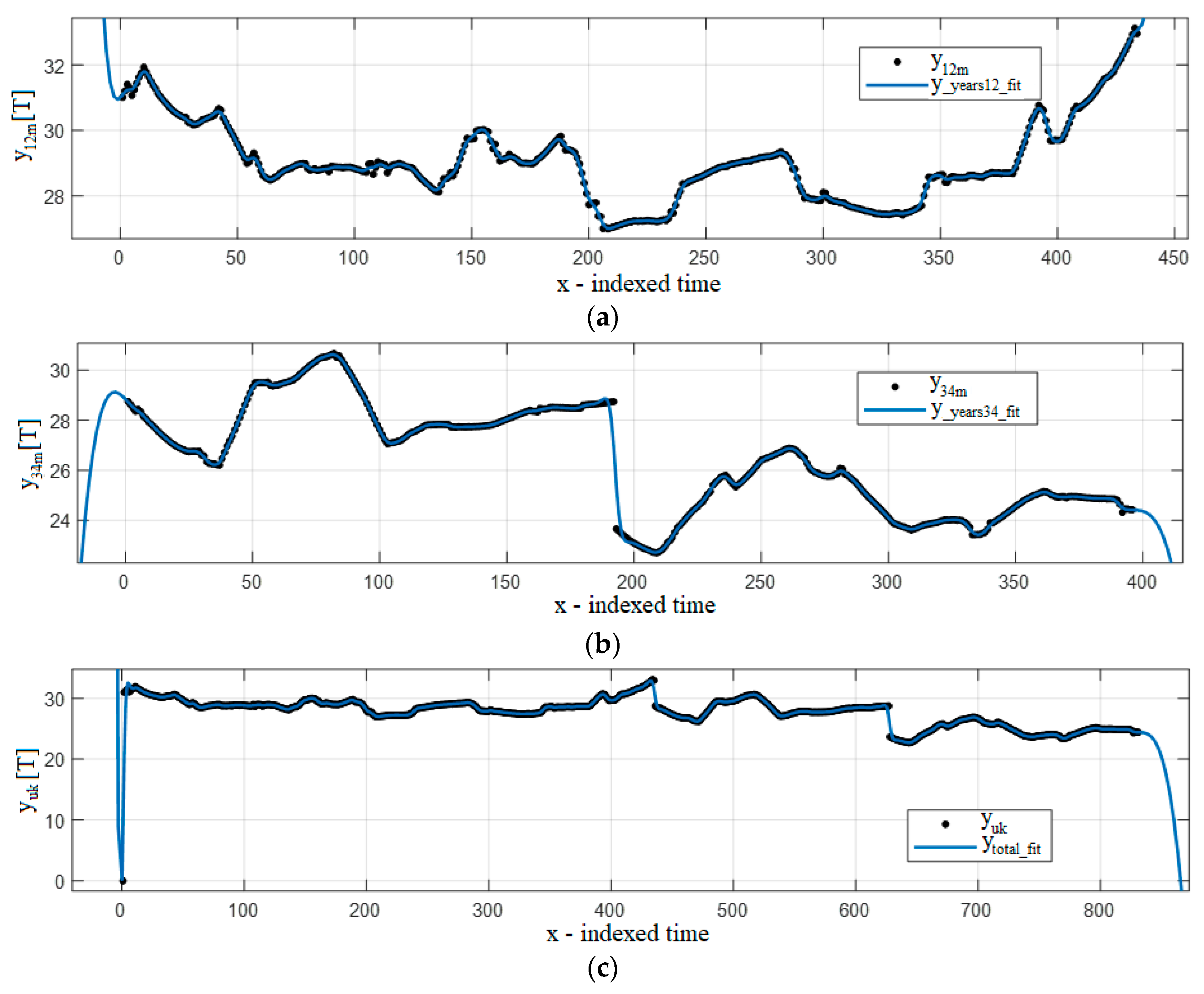
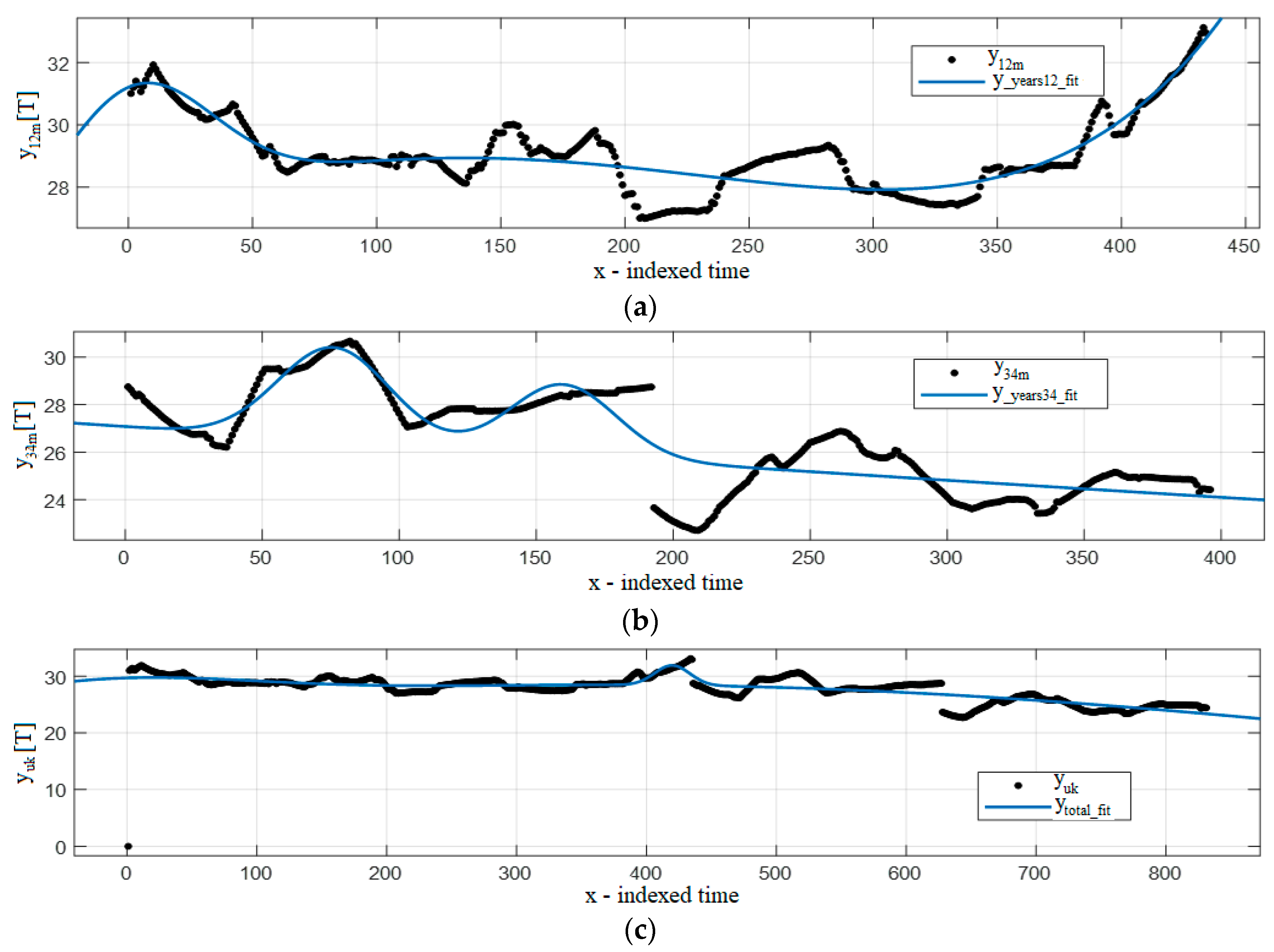
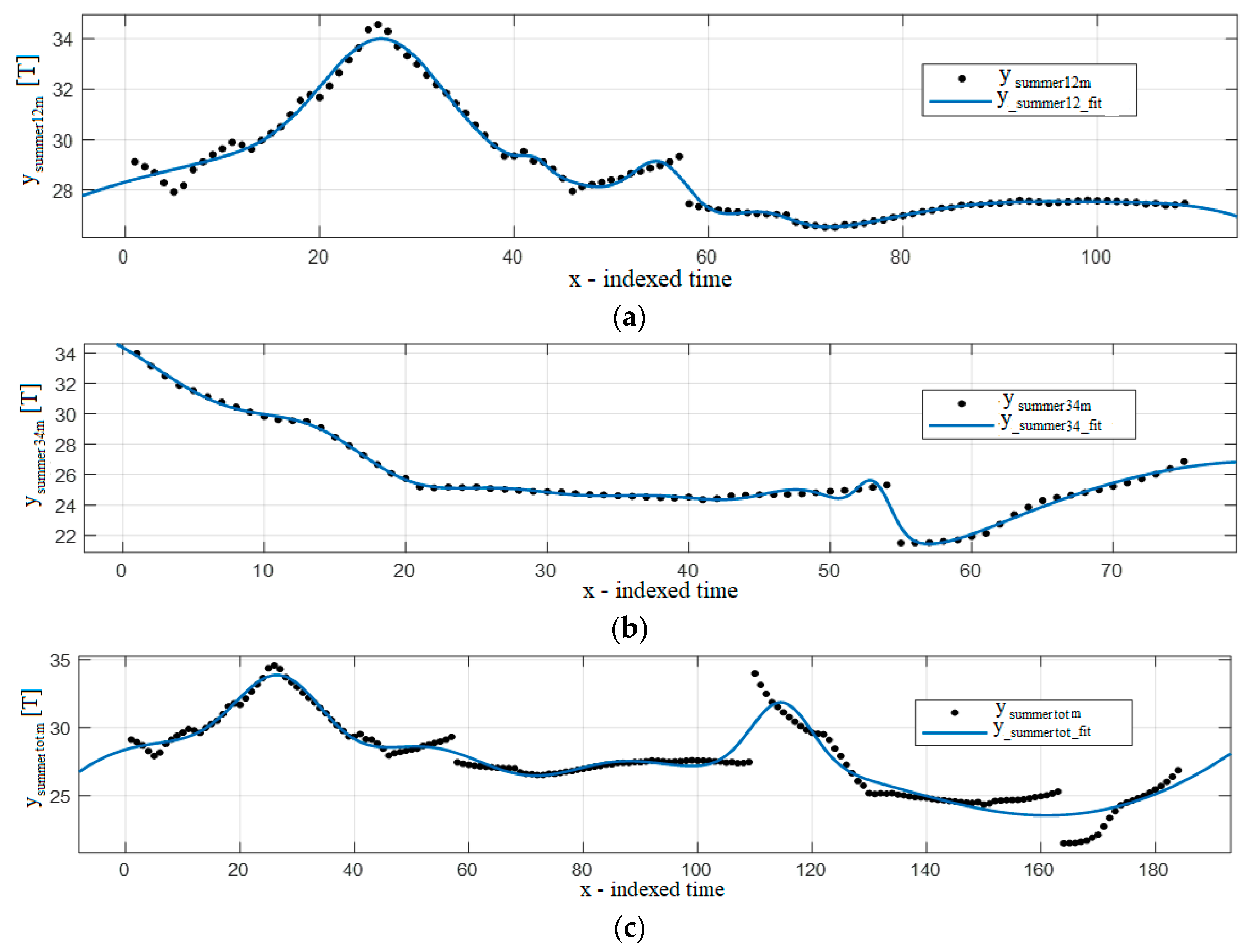
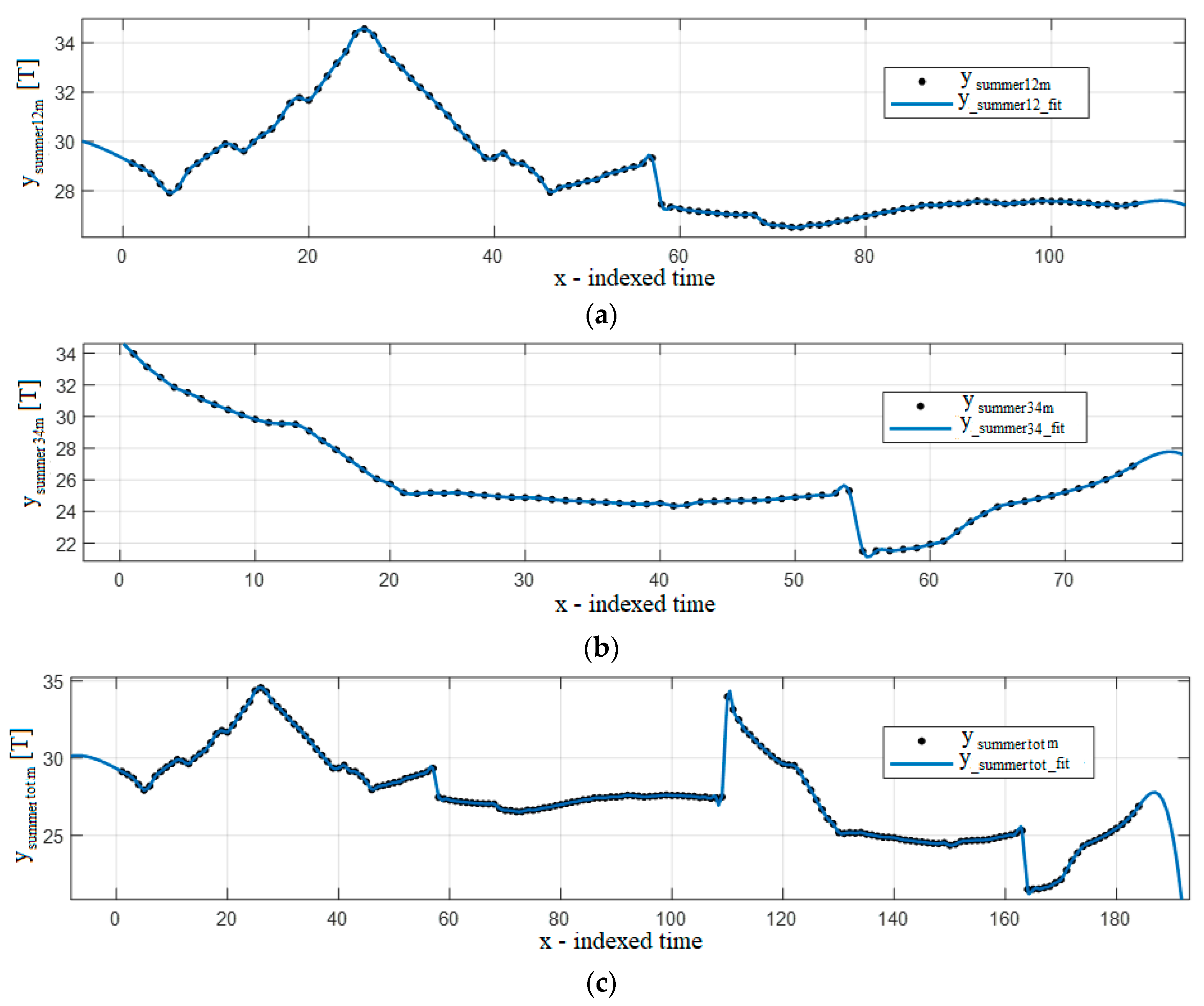
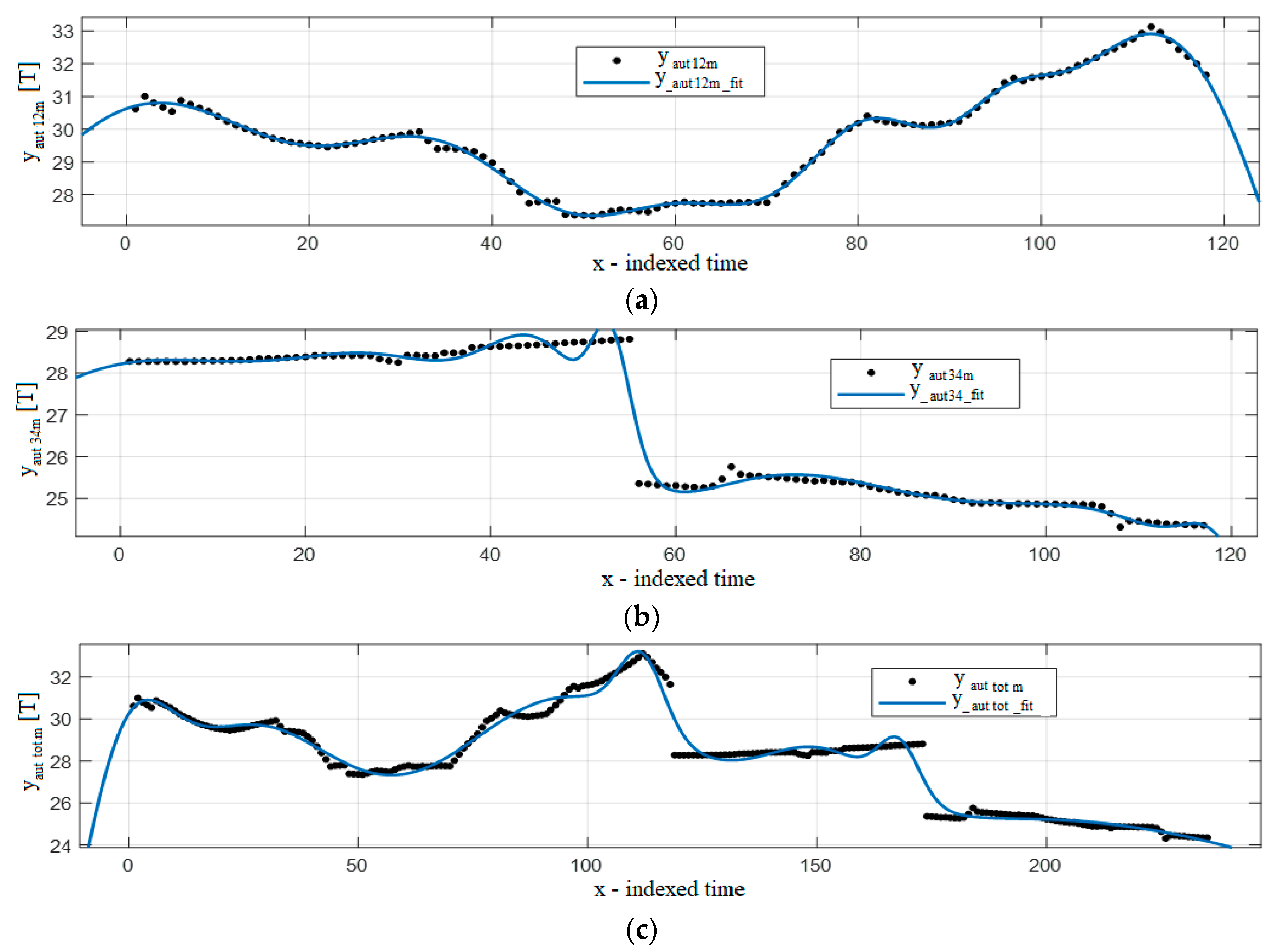
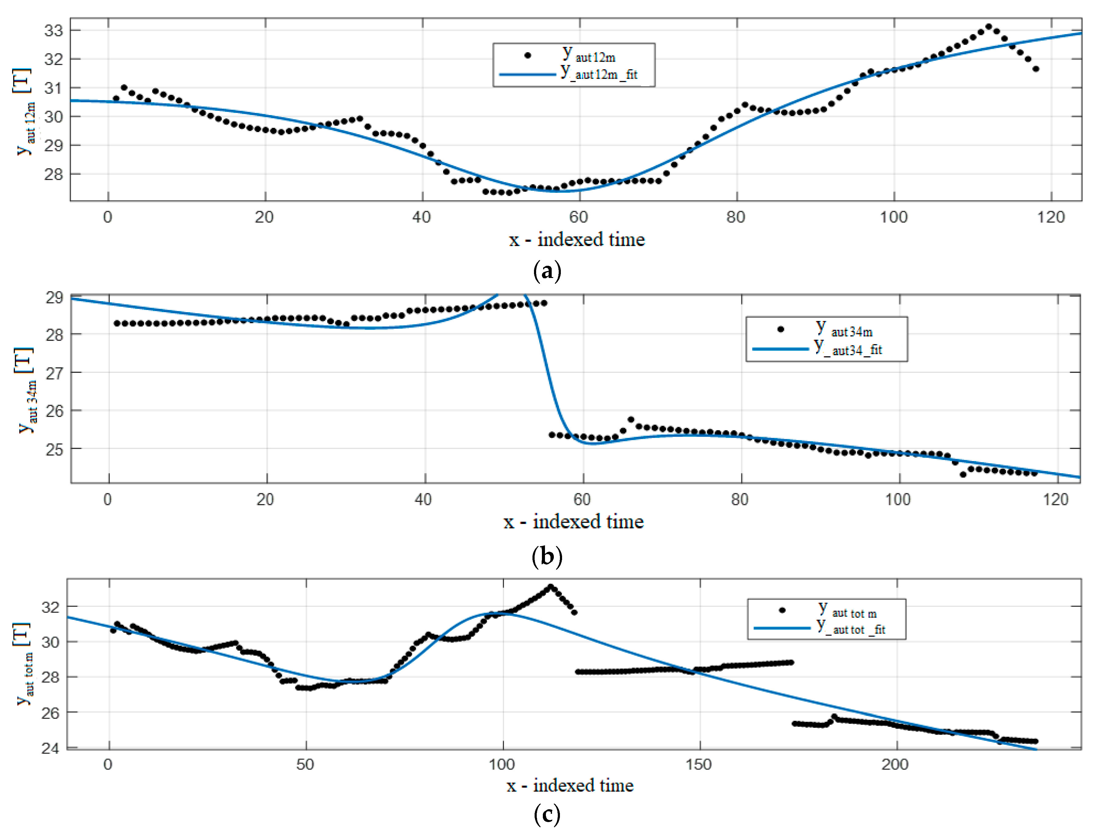
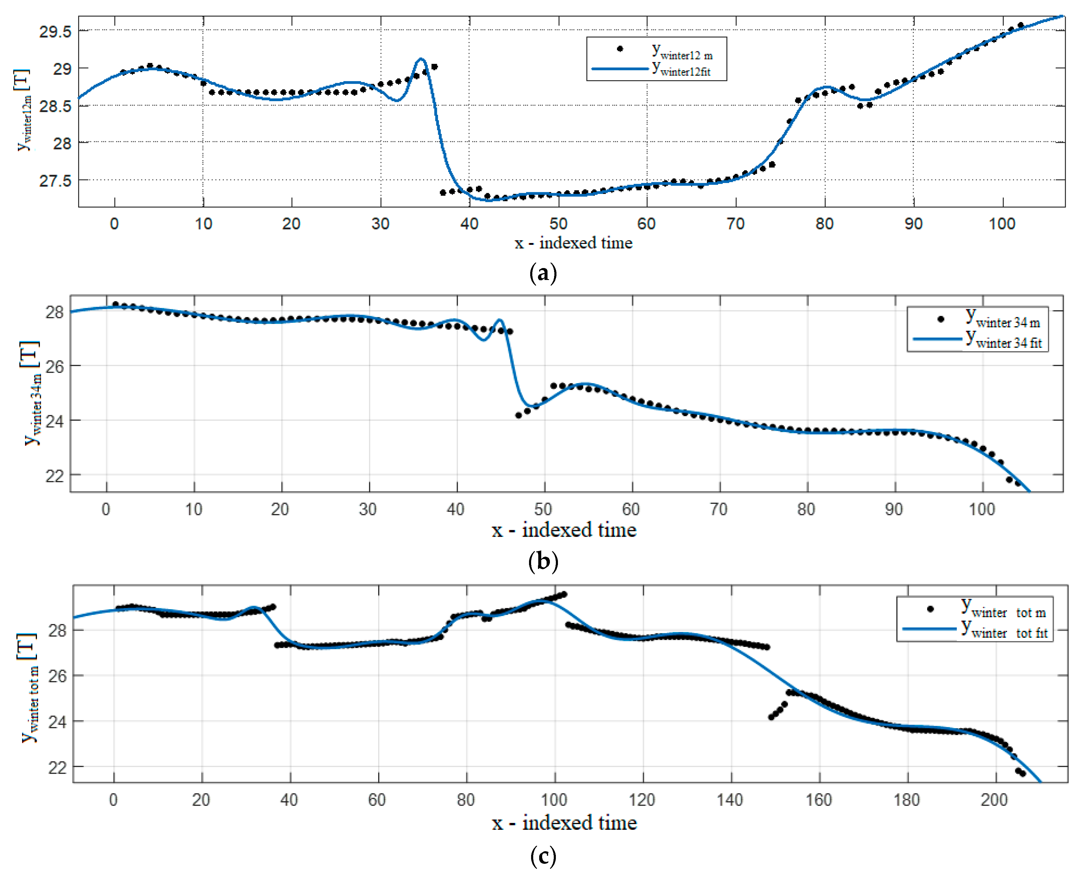

© 2020 by the authors. Licensee MDPI, Basel, Switzerland. This article is an open access article distributed under the terms and conditions of the Creative Commons Attribution (CC BY) license (http://creativecommons.org/licenses/by/4.0/).
Share and Cite
Vujović, I.; Šoda, J.; Kuzmanić, I.; Petković, M. Predicting External Influences to Ship’s Average Fuel Consumption Based on Non-Uniform Time Set. J. Mar. Sci. Eng. 2020, 8, 625. https://doi.org/10.3390/jmse8090625
Vujović I, Šoda J, Kuzmanić I, Petković M. Predicting External Influences to Ship’s Average Fuel Consumption Based on Non-Uniform Time Set. Journal of Marine Science and Engineering. 2020; 8(9):625. https://doi.org/10.3390/jmse8090625
Chicago/Turabian StyleVujović, Igor, Joško Šoda, Ivica Kuzmanić, and Miro Petković. 2020. "Predicting External Influences to Ship’s Average Fuel Consumption Based on Non-Uniform Time Set" Journal of Marine Science and Engineering 8, no. 9: 625. https://doi.org/10.3390/jmse8090625
APA StyleVujović, I., Šoda, J., Kuzmanić, I., & Petković, M. (2020). Predicting External Influences to Ship’s Average Fuel Consumption Based on Non-Uniform Time Set. Journal of Marine Science and Engineering, 8(9), 625. https://doi.org/10.3390/jmse8090625


