The Impact of Tides on the Bay of Biscay Dynamics


Abstract
1. Introduction
2. Ocean Model Simulations and Methodology
2.1. Numerical Model and Set-Up
2.2. Design of the Twin-Experiment
2.3. Methodology
3. Results
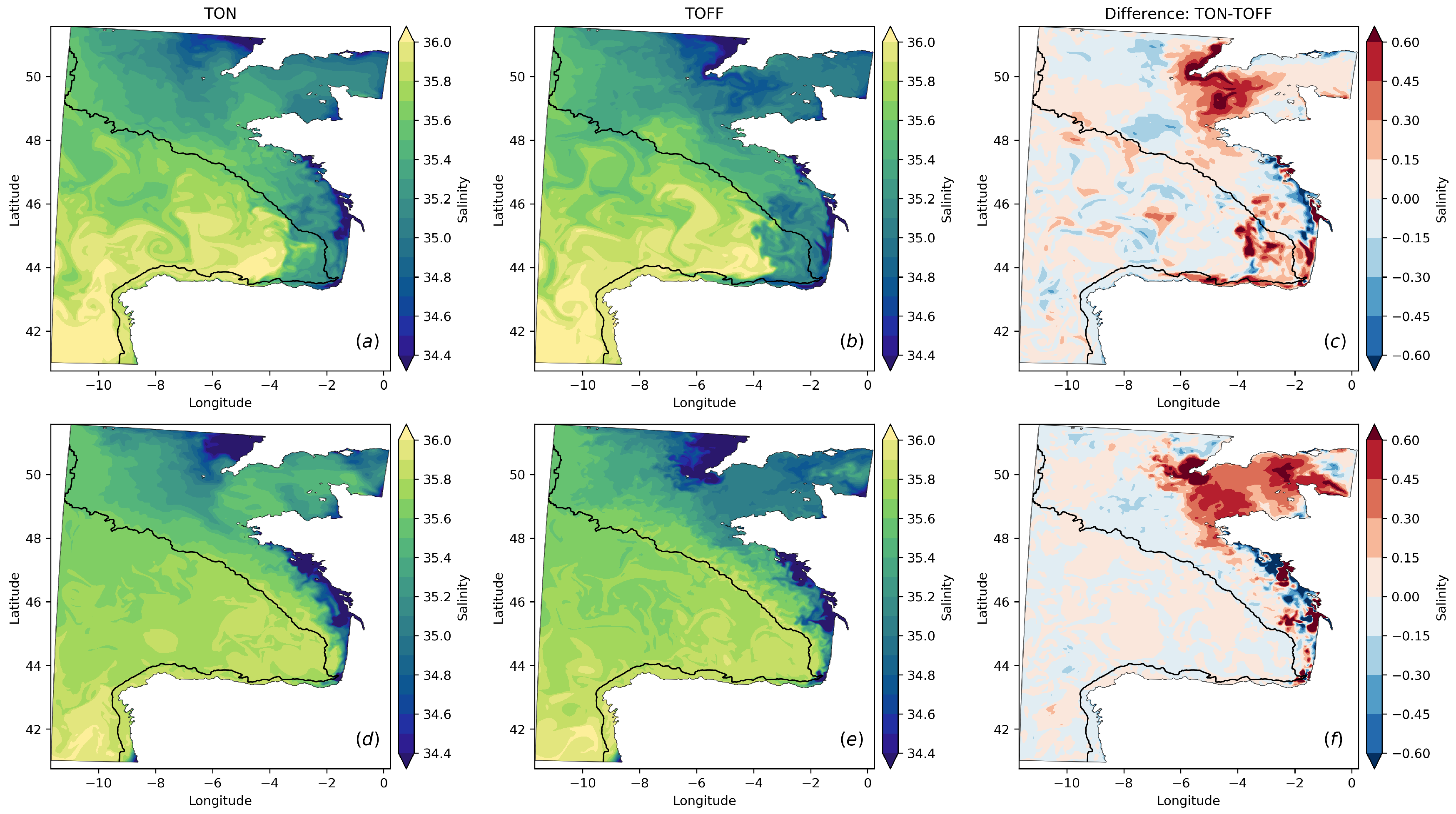
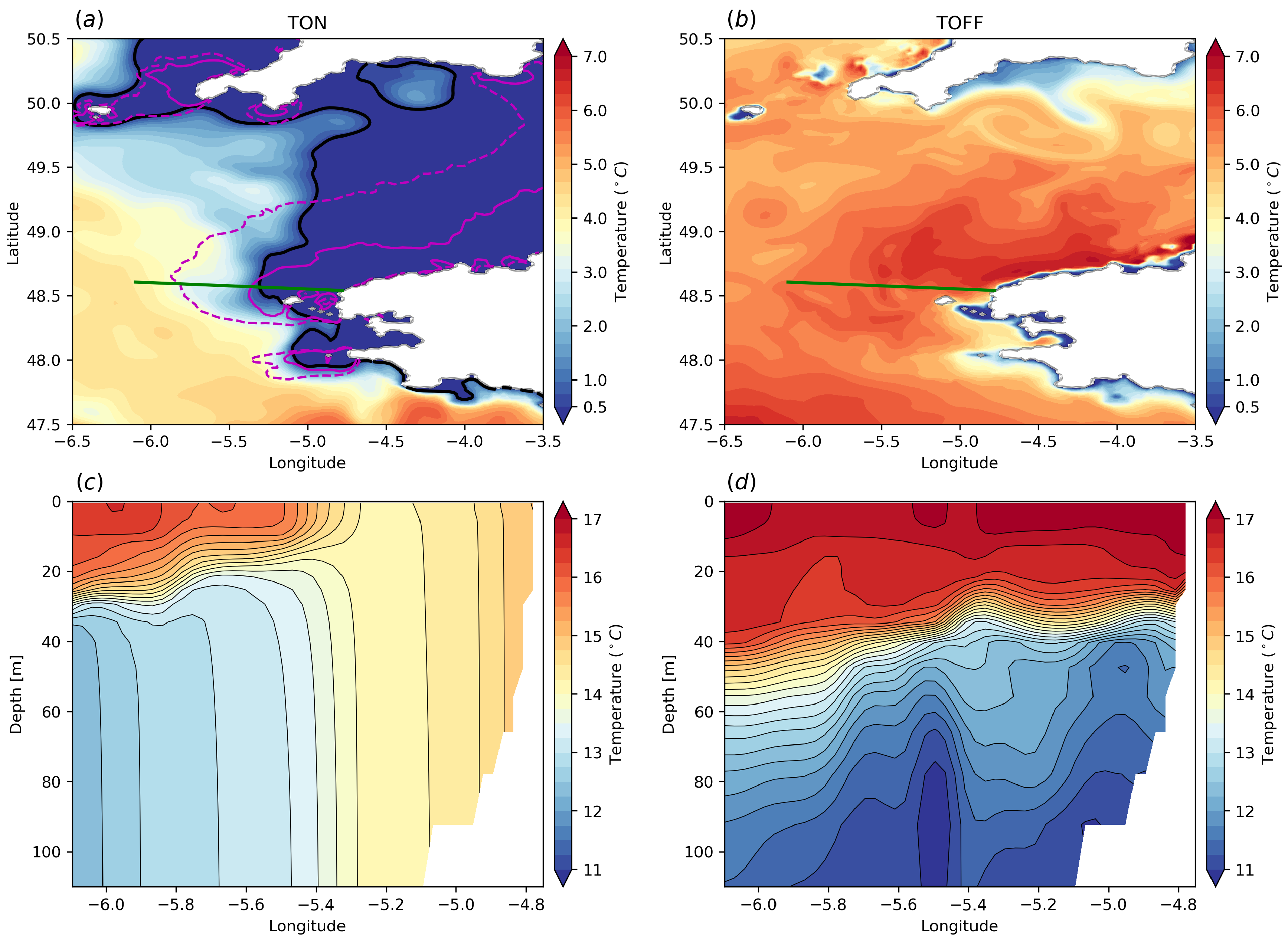
3.1. Distribution of Thermohaline Properties
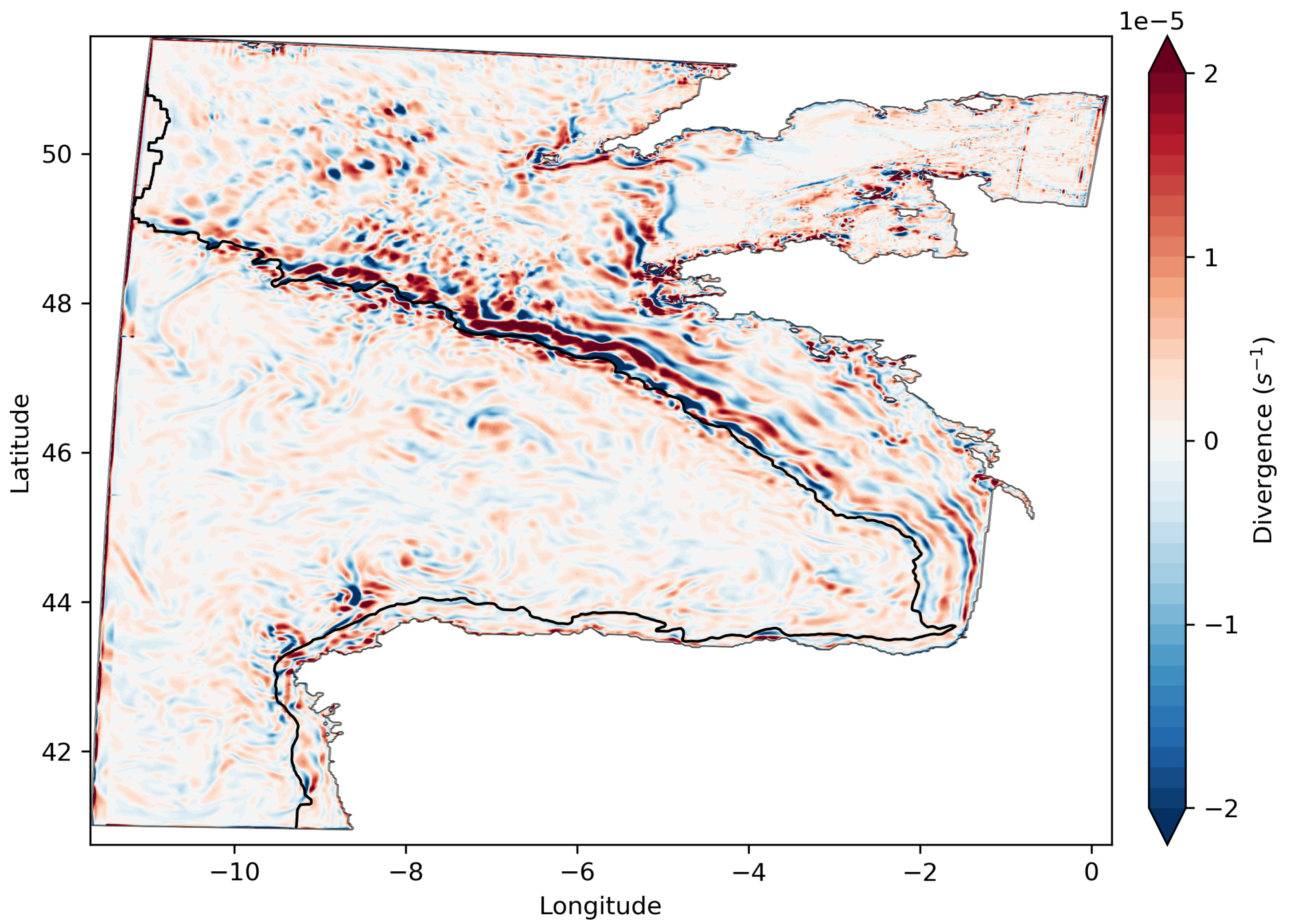
3.2. Relative Vorticity and Divergence
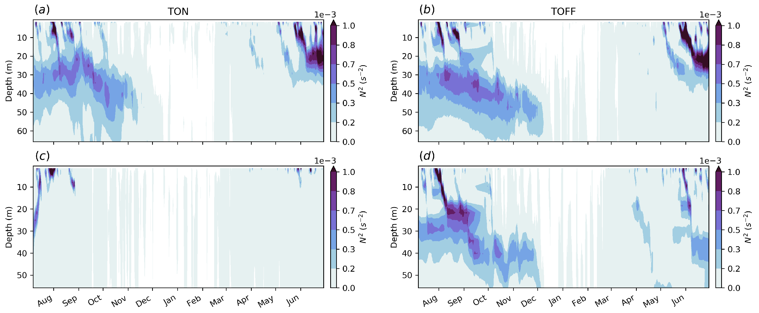
3.3. Vertical Stratification
3.4. Spectral Signatures of Tides
4. Concluding Remarks
Supplementary Materials
Author Contributions
Funding
Acknowledgments
Conflicts of Interest
References
- Gerkema, T.; Lam, F.P.A.; Maas, L.R.M. Internal tides in the Bay of Biscay: Conversion rates and seasonal effects. Deep. Sea Res. Part II Top. Stud. Oceanogr. 2004, 51, 2995–3008. [Google Scholar] [CrossRef]
- Guarnieri, A.; Pinardi, N.; Oddo, P.; Bortoluzzi, G.; Ravaioli, M. Impact of tides in a baroclinic circulation model of the Adriatic Sea. J. Geophys. Res. Ocean. 2013, 118, 166–183. [Google Scholar] [CrossRef]
- Suanda, S.H.; Feddersen, F.; Kumar, N. The Effect of Barotropic and Baroclinic Tides on Coastal Stratification and Mixing. J. Geophys. Res. Ocean. 2017, 122, 10156–10173. [Google Scholar] [CrossRef]
- Stanev, E.V.; Ricker, M. Interactions between barotropic tides and mesoscale processes in deep ocean and shelf regions. Ocean. Dyn. 2020, 70, 713–728. [Google Scholar] [CrossRef]
- Holt, J.; Hyder, P.; Ashworth, M.; Harle, J.; Hewitt, H.T.; Liu, H.; New, A.L.; Pickles, S.; Porter, A.; Popova, E.; et al. Prospects for improving the representation of coastal and shelf seas in global ocean models. Geosci. Model Dev. 2017, 10, 499–523. [Google Scholar] [CrossRef]
- Stammer, D.; Ray, R.D.; Andersen, O.B.; Arbic, B.K.; Bosch, W.; Carrére, L.; Cheng, Y.; Chinn, D.S.; Dushaw, B.D.; Egbert, G.D.; et al. Accuracy assessment of global barotropic ocean tide models. Rev. Geophys. 2014, 52, 243–282. [Google Scholar] [CrossRef]
- Koutsikopoulos, C.; Le Cann, B. Physical processes and hydrological structures related to the Bay of Biscay anchovy. Sci. Mar. 1996, 60, 9–19. [Google Scholar]
- Le Cann, B. Barotropic tidal dynamics of the Bay of Biscay shelf: Observations, numerical modelling and physical interpretation. Cont. Shelf Res. 1990, 10, 723–758. [Google Scholar] [CrossRef]
- Pairaud, I.L.; Lyard, F.; Auclair, F.; Letellier, T.; Marsaleix, P. Dynamics of the semi-diurnal and quarter-diurnal internal tides in the Bay of Biscay. Part 1: Barotropic tides. Cont. Shelf Res. 2008, 28, 1294–1315. [Google Scholar] [CrossRef]
- Pingree, R.D.; Le Cann, B. Structure, strength and seasonality of the slope currents in the Bay of Biscay region. J. Mar. Biol. Assoc. UK 1990, 70, 857–885. [Google Scholar] [CrossRef]
- Garcia-Soto, C.; Pingree, R.D.; Valdés, L. Navidad development in the southern Bay of Biscay: Climate change and swoddy structure from remote sensing and in situ measurements. J. Geophys. Res. 2002, 107, 3118. [Google Scholar] [CrossRef]
- Le Boyer, A.; Cambon, G.; Daniault, N.; Herbette, S.; Le Cann, B.; Marié, L.; Morin, P. Observations of the Ushant tidal front in September 2007. Cont. Shelf Res. 2009, 29, 1026–1037. [Google Scholar] [CrossRef]
- Pingree, R.D.; Le Cann, B. Anticyclonic eddy X91 in the southern Bay of Biscay, May 1991 to February 1992. J. Geophys. Res. Ocean. 1992, 97, 14353–14367. [Google Scholar] [CrossRef]
- Pingree, R.D.; Le Cann, B. Three anticyclonic slope water oceanic eDDIES (SWODDIES) in the Southern Bay of Biscay in 1990. Deep. Sea Res. Part Oceanogr. Res. Pap. 1992, 39, 1147–1175. [Google Scholar] [CrossRef]
- Reverdin, G.; Marié, L.; Lazure, P.; d’Ovidio, F.; Boutin, J.; Testor, P.; Martin, N.; Lourenco, A.; Gaillard, F.; Lavin, A.; et al. Freshwater from the Bay of Biscay shelves in 2009. J. Mar. Syst. 2013, 109–110, S134–S143. [Google Scholar] [CrossRef]
- Porter, M.; Inall, M.E.; Green, J.A.M.; Simpson, J.H.; Dale, A.C.; Miller, P.I. Drifter observations in the summer time Bay of Biscay slope current. J. Mar. Syst. 2016, 157, 65–74. [Google Scholar] [CrossRef]
- Rubio, A.; Caballero, A.; Orfila, A.; Hernández-Carrasco, I.; Ferrer, L.; González, M.; Solabarrieta, L.; Mader, J. Eddy-induced cross-shelf export of high Chl-a coastal waters in the SE Bay of Biscay. Remote. Sens. Environ. 2018, 205, 290–304. [Google Scholar] [CrossRef]
- Akpınar, A.; Charria, G.; Theetten, S.; Vandermeirsch, F. Cross-shelf exchanges in the northern Bay of Biscay. J. Mar. Syst. 2020, 205. [Google Scholar] [CrossRef]
- Baines, P.G. On internal tide generation models. Deep. Sea Res. Part A Oceanogr. Res. Pap. 1982, 29, 307–338. [Google Scholar] [CrossRef]
- Pingree, R.D.; Mardell, G.T.; New, A.L. Propagation of internal tides from the upper slopes of the Bay of Biscay. Nature 1986, 321, 154–158. [Google Scholar] [CrossRef]
- Pingree, R.D.; New, A.L. Structure, seasonal development and sunglint spatial coherence of the internal tide on the Celtic and Armorican shelves and in the Bay of Biscay. Deep. Sea Res. Part I Oceanogr. Res. Pap. 1995, 42, 245–284. [Google Scholar] [CrossRef]
- Pichon, A.; Correard, S. Internal tides modelling in the Bay of Biscay. Comparisons with observations. Sci. Mar. 2006, 70, 65–88. [Google Scholar] [CrossRef]
- Pairaud, I.L.; Auclair, F.; Marsaleix, P.; Lyard, F.; Pichon, A. Dynamics of the semi-diurnal and quarter-diurnal internal tides in the Bay of Biscay. Part 2: Baroclinic tides. Cont. Shelf Res. 2010, 30, 253–269. [Google Scholar] [CrossRef]
- Egbert, G.D.; Ray, R.D. Semi-diurnal and diurnal tidal dissipation from TOPEX/Poseidon altimetry. Geophys. Res. Lett. 2003, 30, 17. [Google Scholar] [CrossRef]
- Pasquet, A.; Szekely, T.; Morel, Y. Production and dispersion of mixed waters in stratified coastal areas. Cont. Shelf Res. 2012, 39–40, 49–77. [Google Scholar] [CrossRef]
- Chevallier, C.; Herbette, S.; Marié, L.; Le Borgne, P.; Marsouin, A.; Péré, S.; Levier, B.; Reason, C. Observations of the Ushant front displacements with MSG/SEVIRI derived sea surface temperature data. Remote. Sens. Environ. 2014, 146, 3–10. [Google Scholar] [CrossRef]
- Schultes, S.; Sourisseau, M.; Le Masson, E.; Lunven, M.; Marié, L. Influence of physical forcing on mesozooplankton communities at the Ushant tidal front. J. Mar. Syst. 2013, 109–110, S191–S202. [Google Scholar] [CrossRef]
- Simpson, J.; Bowers, D. Models of stratification and frontal movement in shelf seas. Deep. Sea Res. Part A Oceanogr. Res. Pap. 1981, 28, 727–738. [Google Scholar] [CrossRef]
- Bowers, D.; Simpson, J. Mean position of tidal fronts in European-shelf seas. Cont. Shelf Res. 1987, 7, 35–44. [Google Scholar] [CrossRef]
- Holt, J.; Umlauf, L. Modelling the tidal mixing fronts and seasonal stratification of the Northwest European Continental shelf. Cont. Shelf Res. 2008, 28, 887–903. [Google Scholar] [CrossRef]
- O’Dea, E.J.; Arnold, A.K.; Edwards, K.P.; Furner, R.; Hyder, P.; Martin, M.J.; Siddorn, J.R.; Storkey, D.; While, J.; Holt, J.T.; et al. An operational ocean forecast system incorporating NEMO and SST data assimilation for the tidally driven European North-West shelf. J. Oper. Oceanogr. 2012, 5, 3–17. [Google Scholar] [CrossRef]
- Yelekçi, Ö.; Charria, G.; Capet, X.; Reverdin, G.; Sudre, J.; Yahia, H. Spatial and seasonal distributions of frontal activity over the French continental shelf in the Bay of Biscay. Cont. Shelf Res. 2017, 144, 65–79. [Google Scholar] [CrossRef]
- Simpson, J.H.; Hunter, J.R. Fronts in the Irish Sea. Nature 1974, 250, 404–406. [Google Scholar] [CrossRef]
- Madec, G. NEMO ocean engine. In Note du Pôle de Modélisation; Institut Pierre-Simon Laplace (IPSL): Paris, France, 2012; 357p. [Google Scholar]
- Maraldi, C.; Chanut, J.; Levier, B.; Ayoub, N.; De Mey, P.; Reffray, G.; Lyard, F.; Cailleau, S.; Drévillon, M.; Fanjul, E.A.; et al. NEMO on the shelf: Assessment of the Iberia-Biscay-Ireland configuration. Ocean. Sci. 2013, 9, 745–771. [Google Scholar] [CrossRef]
- Sotillo, M.G.; Cailleau, S.; Lorente, P.; Levier, B.; Aznar, R.; Reffray, G.; Amo-Baladrón, A.; Chanut, J.; Benkiran, M.; Alvarez-Fanjul, E. The MyOcean IBI Ocean Forecast and Reanalysis Systems: Operational products and roadmap to the future Copernicus Service. J. Oper. Oceanogr. 2015, 8, 63–79. [Google Scholar] [CrossRef]
- Quattrocchi, G.; De Mey, P.; Ayoub, N.; Vervatis, V.D.; Testut, C.E.; Reffray, G.; Chanut, J.; Drillet, Y. Characterisation of errors of a regional model of the Bay of Biscay in response to wind uncertainties: A first step toward a data assimilation system suitable for coastal sea domains. J. Oper. Oceanogr. 2014, 7, 25–34. [Google Scholar] [CrossRef]
- Vervatis, V.; Testut, C.E.; De Mey, P.; Ayoub, N.; Chanut, J.; Quattrocchi, G. Data assimilative twin-experiment in a high-resolution Bay of Biscay configuration: 4DEnOI based on stochastic modeling of the wind forcing. Ocean. Model. 2016, 100, 1–19. [Google Scholar] [CrossRef]
- Large, W.G.; Yeager, S.G. Diurnal to Decadal Global Forcing for Ocean and Sea-Ice Models: The Data Sets and Flux Climatologies; NCAR Technical Note: NCAR/TN-460+STR; University Corporation for Atmospheric Research (UCAR): Boulder, CO, USA, 2004. [Google Scholar] [CrossRef]
- Egbert, G.D.; Bennett, A.F.; Foreman, M.G.G. TOPEX/POSEIDON tides estimated using a global inverse model. J. Geophys. Res. Ocean. 1994, 99, 24821–24852. [Google Scholar] [CrossRef]
- Umlauf, L.; Burchard, H. A generic length-scale equation for geophysical turbulence models. J. Mar. Res. 2003, 61, 235–265. [Google Scholar] [CrossRef]
- Umlauf, L.; Burchard, H. Second-order turbulence closure models for geophysical boundary layers. A review of recent work. Cont. Shelf Res. 2005, 25, 795–827. [Google Scholar] [CrossRef]
- McDougall, T.J. Neutral Surfaces. J. Phys. Oceanogr. 1987, 17, 1950–1964. [Google Scholar] [CrossRef]
- Welch, P. The use of fast Fourier transform for the estimation of power spectra: A method based on time averaging over short, modified periodograms. IEEE Trans. Audio Electroacoust. 1967, 15, 70–73. [Google Scholar] [CrossRef]
- Rocha, C.B.; Chereskin, T.K.; Gille, S.T.; Menemenlis, D. Mesoscale to submesoscale wavenumber spectra in Drake Passage. J. Phys. Oceanogr. 2016, 46, 601–620. [Google Scholar] [CrossRef]
- Le Provost, C.; Fornerino, M. Tidal Spectroscopy of the English Channel with a Numerical Model. J. Phys. Oceanogr. 1985, 15, 1009–1031. [Google Scholar] [CrossRef]
- Donlon, C.J.; Martin, M.; Stark, J.; Roberts-Jones, J.; Fiedler, E.; Wimmer, W. The Operational Sea Surface Temperature and Sea Ice Analysis (OSTIA) system. Remote. Sens. Environ. 2012, 116, 140–158. [Google Scholar] [CrossRef]
- Timko, P.G.; Arbic, B.K.; Hyder, P.; Richman, J.G.; Zamudio, L.; O’Dea, E.; Wallcraft, A.J.; Shriver, J.F. Assessment of shelf sea tides and tidal mixing fronts in a global ocean model. Ocean. Model. 2019, 136, 66–84. [Google Scholar] [CrossRef]
- Kelly-Gerreyn, B.A.; Hydes, D.J.; Jégou, A.M.; Lazure, P.; Fernand, L.J.; Puillat, I.; Garcia-Soto, C. Low salinity intrusions in the western English Channel. Cont. Shelf Res. 2006, 26, 1241–1257. [Google Scholar] [CrossRef][Green Version]
- Lelong, M.P.; Kunze, E. Can barotropic tide–eddy interactions excite internal waves? J. Fluid Mech. 2013, 721, 1–27. [Google Scholar] [CrossRef]


© 2020 by the authors. Licensee MDPI, Basel, Switzerland. This article is an open access article distributed under the terms and conditions of the Creative Commons Attribution (CC BY) license (http://creativecommons.org/licenses/by/4.0/).
Share and Cite
Karagiorgos, J.; Vervatis, V.; Sofianos, S. The Impact of Tides on the Bay of Biscay Dynamics. J. Mar. Sci. Eng. 2020, 8, 617. https://doi.org/10.3390/jmse8080617
Karagiorgos J, Vervatis V, Sofianos S. The Impact of Tides on the Bay of Biscay Dynamics. Journal of Marine Science and Engineering. 2020; 8(8):617. https://doi.org/10.3390/jmse8080617
Chicago/Turabian StyleKaragiorgos, John, Vassilios Vervatis, and Sarantis Sofianos. 2020. "The Impact of Tides on the Bay of Biscay Dynamics" Journal of Marine Science and Engineering 8, no. 8: 617. https://doi.org/10.3390/jmse8080617
APA StyleKaragiorgos, J., Vervatis, V., & Sofianos, S. (2020). The Impact of Tides on the Bay of Biscay Dynamics. Journal of Marine Science and Engineering, 8(8), 617. https://doi.org/10.3390/jmse8080617