UAV Trajectory Planning in a Port Environment

Abstract

In many situations, the trajectory of an unmanned aerial vehicle (UAV) is very likely to deviate from the initial path generated by a path planning algorithm. This is in fact due to the existence of dynamic constraints of the UAV. In order to reduce the degree of such a deviation, this research introduces a trajectory planning algorithm, the objective of which is to minimize distance while maintaining security. The algorithm first develops preprocess trajectory points by constructing isosceles triangles then, on the basis of a minimum snap trajectory method, it applies a corridor constraint to an optimization objective function, while the deviation evaluation function is established to quantitatively evaluate the deviation distance. A series of experiments were carried out in a simulation environment with a simplified quay crane model. The results show that the proposed method not only optimizes the time and length of the generated trajectory, but also reduces the average deviation distance by 88.7%. Moreover, the generated trajectory can be well tracked by the UAV through qualitative and quantitative analysis. Overall, the experiments show that the proposed method can generate a higher UAV trajectory quality.

1. Introduction

A port environment is a relatively self-executing and complex transportation system, in which the role of the quay crane is to achieve the efficient transportation of goods between land and sea [1]. Due to frequent operations of the quay crane, a series of damages, such as cracks and rust, may affect the service life of the machinery. Therefore, a quay crane should be maintained regularly and properly. Usually, maintenance operations and inspections are carried out by specialized personnel on the quay crane, which is time-consuming and laborious work. This not only requires frequent long-term shutdowns of the equipment, but also generates unforeseen dangers to the workers [2]. Recently, UAVs have been widely used in the detection industry because of their high maneuverability and operability and their lack of reliance on network infrastructures [3]. The purpose of a UAV trajectory planning is to quickly generate a collision-free trajectory from the starting position to the goal position under some given constraints.

Previous related works have implemented UAV trajectory planning in two steps. Firstly, a set of collision-free waypoints are generated by a path planning algorithm, and then an optimized trajectory is generated. A series of recent works have put forward a large number of path planning algorithms.

Chen and Luo introduced an artificial potential field method updated by optimal control theory that generates relatively short and smooth trajectories [4]. However, defining the potential field precisely is a difficult task. Meng and Xin developed a solution that combines a simulated annealing algorithm with a genetic algorithm to deal with the local optimal solution problem [5]. However, for large-scale environments the method has not proven to be efficient. Wang and Zhou presented an improved quantum particle swarm optimization, but the approach is mainly oriented to autonomous underwater vehicles [6]. Cheng and Cheng introduced a path planning method based on an A* algorithm, which can improve search efficiency in a 3D environment [7]. However, the path generated by this method is a broken-line path. The A* algorithm and postprocessing method can generate collision-free paths between adjacent monitoring points [8], but the generated path is still made of broken-line paths; therefore the acceleration of the UAV at each corner is likely to have a sudden change, which greatly reduces the efficiency of the UAV and wastes its energy [9]. Therefore, after the waypoints are generated, a trajectory optimization is still needed to generate a smooth trajectory.

There have been many nonlinear optimization techniques for trajectory optimization, such as the direct collocation [10] and shooting methods [11], which can be used to generate optimal local paths. However, these methods are also computationally intensive and may require accurate analytical representations of environmental constraints in order to efficiently compute cost gradients with respect to the identified obstacles. When these constraints are represented in the form of an occupancy map, these restrictions make these methods almost impractical. Explicit optimization can quickly generate trajectory solutions in cluttered environments. The minimum snap trajectory is an appropriate choice for a quadrotor UAV with a high degree of freedom, because the motor command and attitude acceleration of the UAV are proportional to the fourth derivative of the trajectory [12]. Minimum snap trajectory ensures the quality of onboard sensor measurements while avoiding sudden or excessive control inputs. However, due to the constraints of the parameter matrix in the quadratic programming, the above optimization method cannot deal with multisegmented, high-order polynomial trajectories in a large range [13]. The unconstrained quadratic programming (UQP) is obtained by a technique of substitution, and the time distribution is optimized by a gradient descent method [14]. The joint polynomial trajectory optimization method can solve the problems of a relatively large number of segment trajectories without calculation difficulty [15], but the generated trajectory deviates from the planned straight-line path.

In order to solve the above problems, and by retaining a joint polynomial trajectory optimization, the research developed in this paper firstly introduces a method in which a planned straight-line path is first preprocessed in order to suppress the deviation distance. Secondly, corridor constraints are added to the optimization objective function in order to generate the optimized trajectory. Finally, a deviation evaluation function is established to qualitatively analyze the effect of the optimization process. The rest of the paper is structured as follows: Section 2 presents the trajectory planning problem. Section 3 develops the motion model and control of a UAV. Section 4 introduces the principles behind the piecewise polynomials’ joint trajectory optimization, while Section 5 studies the deviation constraints. Section 6 presents the simulation experiments, while Section 7 concludes the paper.

2. Trajectory Planning Problem

A quay crane is a complex mechanical system. Due to frequent operation, some parts are prone to damage. Fatigue failure is one of the main forms of a quay crane’s metal structure failure. The fatigue crack growth life estimation method is generally used to evaluate and plan maintenance operations. The life prediction of the crane’s metal structure can be regarded as an initial crack with a certain time from propagation to fracture. An initial crack should be identified by physical detection, which is the target of a UAV operating on a quay crane. First of all, according to the experience of experts in the field, a series of vulnerable points can be obtained. Given a series of detection points, the objective of a trajectory planning is to generate a smooth trajectory that satisfies motion constraints. A simplified and representative quay crane model and vulnerable points are shown in Figure 1, where the black dots indicate the parts of the quay crane that are prone to damage. Due to the symmetry of the overall structure of the quay crane, L and R are the set of vulnerable points on the left and right sides of the quay crane respectively, as labeled in Figure 1 and shown in

Table 1. Vulnerable points of a quay crane.

L	1	2	3	4	5	6	7	8	9	10	11	12	13	14	15	16	17	18	19	20
R	1	2	3	4	5	6	7	8	9	10	11	12	13	14	15	16	17	18	19	20

.

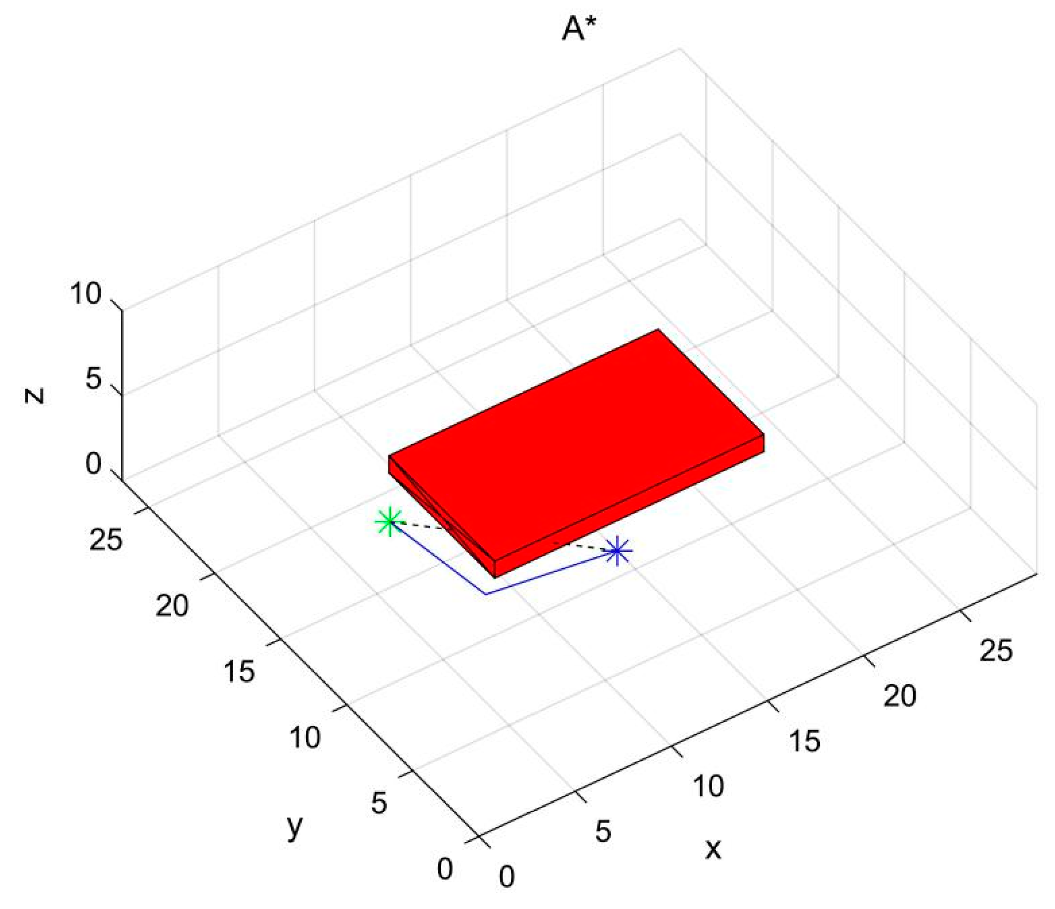
When the UAV flies over a quay crane, the quay crane is both a detected target and an obstacle in the environment. In order to prevent collisions caused by human misjudgments, the A* algorithm is also used to generate an optimal path without collision between adjacent waypoints. In the case of human misjudgment, the generation of collision-free waypoints by the A* algorithm is shown in Figure 2. The blue and cyan points represent the points given by the experts in the field. The straight line between the two points will encounter obstacles, as shown by the black dotted line. The blue path is a collision-free path generated by the A* algorithm.

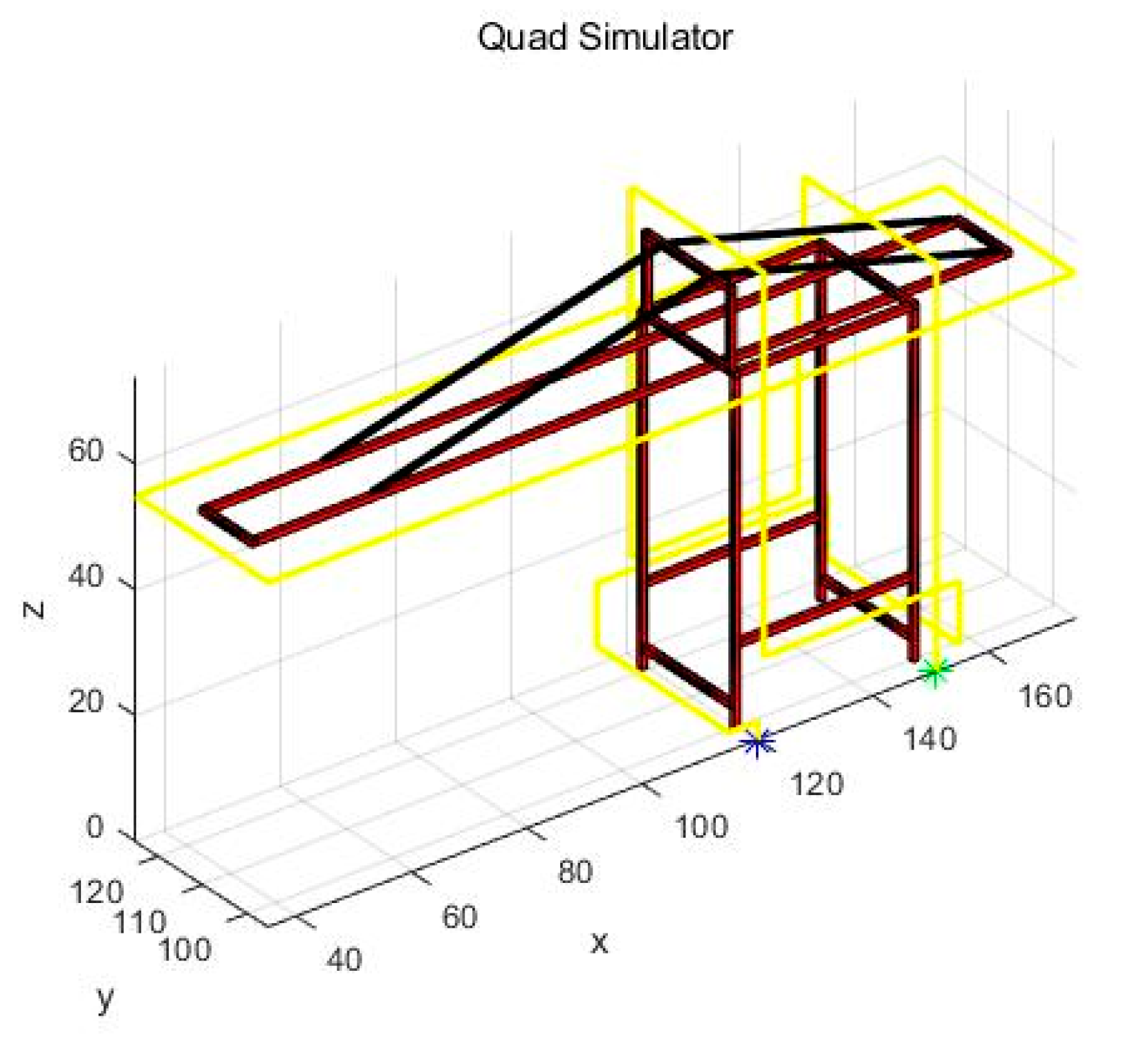
The given waypoints are optimized detection points, and the structure of the quay crane is regular, so the path generated by the A* algorithm is an optimized UAV detection path. The simulation model of the detection route and the quay crane are shown in Figure 3, in which the length, width, and height of the overall size of the model are 132, 22, and 70 m, respectively. The blue and green points represent the starting point coordinates (120, 95, 0) and the ending point coordinates (151, 95, 0), respectively, and the yellow line shows the ideal detection route.

However, when the UAV is flying along a straight-line path, there will be a greater acceleration at each corner, which not only has high requirements of the motion characteristics of the UAV, but also greatly increases the energy loss. In the monitoring task, trajectory planning not only needs to generate a feasible trajectory, but also needs to consider the quality of the data obtained in the monitoring. First of all, the clarity and consistency of the captured image affect the quality of the detection. Therefore, in order to keep the camera parallel to the detection target, the generated trajectory should be as close as possible to the planned straight-line path.

3. Motion Model and Control of UAV

A previously introduced model of UAV motion only allows it to have a very small pitch and roll angle during flight, which limits the motion of the UAV [16]. In order to make better use of UAV’s full dynamic motion, the motion equation of a UAV is described as follows:

$$m\ddot{r}=-mg{z}_W+u_1{z}_B$$

(1)

$${\dot{\omega }}_{BW}=I^{-1}\left[-{\omega }_{BW}\times I{\omega }_{BW}+\left[\begin{array}{c}{u}_2\\ u_3\\ u_4\end{array}\right]\right]$$

(2)

The differential flatness of this equation of motion has been shown in a related work [17]. In this equation, $m$ is the mass of the UAV; $g$ is the acceleration of gravity; $\ddot{r}$ is the second derivative of the position vector of a three-dimensional coordinate; and $u_1$, $u_2$, $u_3$, and $u_4$ denote the total thrust force and the three total torques around the three coordinate axes in the body coordinates, respectively. $z_W$ denotes the unit vector representing the direction of gravity in inertial coordinates, $z_B$ is the unit vector representing the direction of rotor thrust force in the body coordinate system, and $I$ is the rotational inertia vector of the UAV along the coordinate axis in the body coordinate system. ${\omega }_{BW}$ is the angular velocity of the UAV in the body coordinate system.

Any smooth trajectory, with a reasonable bounded derivative, in a flat output space can be tracked by a quadrotor UAV with an under-actuated system [18]. Let $\sigma$ from the trajectory denote the desired input of the controller:

$$\sigma ={[x,y,z,\psi ]}^T$$

(3)

where $r={[x,y,z]}^T$ are the coordinates of the center of mass in the world coordinate system, and $\psi$ is the yaw angle of the UAV. The thrust force and torques output by the controller are as follows:

$$u_1=(-K_p{e}_p-K_v{e}_v+mg{z}_W+m{\ddot{r}}_T)·z_B$$

(4)

$${[u_2,u_3,u_4]}^T=-K_R{e}_R-K_{\omega }{e}_{\omega }+{\omega }_{BW}\times I{\omega }_{BW}-I({\stackrel{⌢}{\omega }}_{BW}{R}^T{R}_d{\omega }_{BW}^d-R^T{R}_d{\dot{\omega }}_{BW}^d)$$

(5)

where $e_p$, $e_v$, $e_R$, and $e_{\omega }$ denote the error vectors in position, velocity, attitude, and angular acceleration, respectively. $K_p$, $K_v$, $K_R$, and $K_{\omega }$ denote the related control gains. $R_d$ is the rotation matrix that represents the desired UAV.

4. Piecewise Polynomials’ Joint Trajectory Optimization

For a quadrotor UAV, a trajectory segment between two waypoints in a flat output space is denoted by $P(t)$. The polynomial function $P(t)$ of the trajectory segment is as follows:

$$P(t)=p_n{t}^n+p_{n-1}{t}^{n-1}+\dots +p_{1}t+p_0$$

(6)

where $p_i(i=0,1,\dots ,n)$ is a coefficient of the unknown polynomial function. $t\in [0,\tau ]$, and $\tau$ is the allocated time for each trajectory. The objective function of the minimum snap polynomial trajectory optimization is as follows:

$$J={\displaystyle {\int }_0^{\tau }{P}^{(4)}{(t)}^2}dt=\mathrm{p}Q\mathrm{p}$$

(7)

where $\mathrm{p}$ is the vector of polynomial coefficient of a segment trajectory, $Q$ is the cost matrix, and $\tau$ is the time allocated to the segment trajectory. It can be obtained that all piecewise polynomials are jointly optimized, and the cost function of the joint optimization is as follows:

$$J_q={\left[\begin{array}{c}{b}_1\\ ⋮\\ b_M\end{array}\right]}^T{\left[\begin{array}{ccc}{A}_1& & \\ & \ddots & \\ & & A_M\end{array}\right]}^{-T}\left[\begin{array}{ccc}{Q}_1& & \\ & \ddots & \\ & & Q_M\end{array}\right]{\left[\begin{array}{ccc}{A}_1& & \\ & \ddots & \\ & & A_M\end{array}\right]}^{-1}\left[\begin{array}{c}{b}_1\\ ⋮\\ b_M\end{array}\right]$$

(8)

where, using the technique of substitution, $A^{-1}b$ is used to replace the coefficient vector $\mathrm{p}$, which is both unknown and constrained, and the value of $M$ can reach about 50 without the problem of insufficient computing power.

5. Deviation Constraints

5.1. Deviation Model

When the trajectory optimization is performed, the trajectory is likely to deviate greatly from the straight-line path, so the probability of the trajectory hitting an obstacle may increase, which will cause the number of collision detections to increase. Let us use several waypoints in Figure 1 as an example. The deviation between the trajectory and the straight-line path is shown in Figure 4. The red points show the waypoints used for detecting vulnerable points L13, L12, R12, and R13, while the blue line indicates the ideal line of the detection path. Finally, the color curve is the trajectory generated by the minimum stop trajectory method.

It can be seen that the generated trajectory deviates from the straight-line path. When the generated trajectory detects a collision, the algorithm adds control points to the original waypoints and then re-optimizes the trajectory until a collision-free trajectory is generated. This means that as the deviation distance increases, the computation time required to generate the trajectory may increase exponentially.

5.2. Preprocessing

Due to the existence of angles, the trajectory of the generator polynomial will inevitably deviate from the initial straight-line path. Let us first preprocess the waypoints. Taking two adjacent straight-line segments as two vectors according to the direction of flight, a simple analysis can be obtained: the smaller the direction change angle between the two vectors, the easier it is to generate a smooth trajectory. For example, if the change of direction between each straight-line segment is very small, assuming that it can be ignored, then the generated trajectory and straight line can basically coincide. Using this principle, we preprocess a given waypoint.

The preprocessing principle is shown in Figure 5. The specific method is to build an isosceles triangle with the supplementary angle of the directional angle as the top angle. For the purpose of ensuring that the bottom edge does not collide, replace the two waists with this bottom edge.

Define the angle of direction change between adjacent path segment vectors as $\beta$,

$$\beta =\arccos \frac{(r_{i+2}-r_{i+1})·(r_{i+1}-r_i)}{\left|r_{i+2}-r_{i+1}\right|\left|r_{i+1}-r_i\right|}$$

(9)

$$l=\frac{d}{2\cos (\beta /2)}$$

(10)

where $r_i$ represents the coordinates of the $i$-th waypoints, $d$ is a constant, and $l$ represents the waist length of the isosceles triangle (DB and BE in Figure 5). The coordinates of the two points D and E can be obtained, so the new path segments of $\mathrm{A}\to \mathrm{D}\to \mathrm{E}\to \mathrm{C}$ replace the original path segments of $\mathrm{A}\to \mathrm{B}\to \mathrm{C}$. Finally, a group of preprocessed waypoints are obtained by sampling at the midpoint of each path segment.

5.3. Corridor Constraints

In order to limit the deviation of the trajectory and the straight line, corridor constraints were added in the above optimization process. Define $t_i$ as a unit time vector from path point $r_i$ to point $r_{i+1}$. Define $d_i(t)$ as the vertical distance vector from path point $r_i$ to point $r_{i+1}$:

$$d_i(t)=(r_T(t)-r_i)-((r_T(t)-r_i)·t_i)t_i$$

(11)

The corridor width ${\delta }_i$ under the infinite norm is defined as follows for each corridor:

$${\Vert d_i(t)\Vert }_{\infty }\le {\delta }_i\mathrm{while}{t}_i\le t\le t_{i+1}$$

(12)

The corridor constraint and unconstrained quadratic planning for a specific point are combined as

$$\left|d_i(t_t+\frac{j}{1+n_c}(t_{i+1}-t_i))\right|\le {\delta }_i$$

(13)

where $j$ represents the point where the constraint is to be added is the $j$-th sampling point. $n_c$ is the number of sampling points. ${\delta }_i$ is the width of the corridor constraints.

In addition to corridor constraints, the allocation time of each trajectory segment also has a crucial impact on the trajectory segment. Therefore, first randomly allocate time as 1~4 s, which is obtained according to the experimental environment, and then use gradient optimization to find the optimal time solution. Then find the parameters of the trajectory segment, so as to obtain the specific polynomial trajectory function.

5.4. Evaluation Function

Since the trajectory generated above will deviate from the straight-line path, the following evaluation function is established in order to describe the degree of deviation between them. Use $x(P)=(r_1,\dots ,r_p)$ to represent the planned waypoint and $x(T)=(v_1,\dots ,v_q)$ to represent the generated trajectory points. When $p\ne q$, several points should be inserted in the middle of the straight-line segment to correspond one-to-one with the points on the trajectory segment. The principle of establishing the evaluation function is shown in Figure 6, where the black curve is the generated trajectory and the straight line is the planned straight-line path.

The expression of the degree of deviation is as follows:

$${\delta }_{dF}=\frac{1}{q}{\displaystyle \sum _{i=1}^{q}d(P(i),T(i))}=\frac{1}{q}{\displaystyle \sum _{i=1}^q\sqrt{{(r_i-v_i)}^2}}$$

(14)

The value represents the average value of the sum of the Euclidean distances between all corresponding points and represents the degree of deviation of the trajectory from the straight-line path. It can be seen that when ${\delta }_{dF}=0$, $P=T$; this means that the trajectory and the straight-line path completely coincide.

6. Simulation Experiments

6.1. Simulation Principles

All simulation experiments were performed by MATLAB on a laptop with a 2.20 GHz Intel i5 CPU (Intel, Santa Clara, CA, USA). Because the results of each experiment are different, and in order to ensure the rationality of the comparison results, we carried out five experiments on each of the two methods. The test results are shown in

Table 2. Data comparison of five test results for each of the two methods.

	Number of Collisions Detected	${\mathit{\delta }}_{\mathit{d}\mathit{F}} \left(\mathbf{m}\right)$	Maximum Deviation Distance (m)	Trajectory Length (m)
UQP Method Test 1	1	5.36	31.47	1019.70
UQP Method Test 2	1	5.25	24.64	1050.10
UQP Method Test 3	3	5.28	24.43	1044.30
UQP Method Test 4	2	5.03	42.31	1029.90
UQP Method Test 5	4	4.24	34.19	998.90
Our Method Test 1	2	1.00	6.46	876.04
Our Method Test 2	2	1.20	11.15	850.69
Our Method Test 3	0	0.87	9.32	824.12
Our Method Test 4	0	0.60	4.27	807.29
Our Method Test 5	0	1.17	22.47	812.88

. Furthermore, a few additional statistics from the derived data, such as average and maximum values at different times and comparison results are shown in

Table 3. Comparison of average and maximum values of five experimental results.

	Number of Collisions Detected	${\mathit{\delta }}_{\mathit{d}\mathit{F}}\left(\mathbf{m}\right)$	Maximum Deviation Distance (m)	Trajectory Length (m)
Average Value of UQP	2.2	5.03	31.41	1028.58
Average Value of Our Method	0.8	0.97	10.73	834.01
Maximum Value of UQP	4	5.36	42.31	1050.10
Maximum Value of Our Method	2	1.20	22.47	876.04

. The data in these two tables show that the proposed method performs better according to these indicators, especially regarding the deviation distance. This subsection presents a detailed comparison of a pair of optimal experimental results.

In the simulation environment, the trajectories generated by the unconstrained quadratic programming (UQP) method and the proposed method were compared, and the results are shown in Figure 7. The blue and green points are the starting point coordinates (120, 95, 0) and the ending point coordinates (151, 95, 0), respectively, and the yellow straight line represents the collision-free detection path generated by the A* algorithm. The colored curve represents the generated trajectory segments. It can be seen from the trajectory generated by the proposed method that it is significantly better than the that of the UQP method. At the same time, the analysis was carried out by the following three evaluation indicators. The comparison of results of quantitative analysis of the two methods are shown in

Table 4. Comparison of quantitative analysis results of the two methods.

	Number of Collisions Detected	${\mathit{\delta }}_{\mathit{d}\mathit{F}}\left(\mathbf{m}\right)$	Maximum Deviation Distance (m)	Trajectory Length (m)
UQP Methods	1	5.25	24.64	1050.10
Proposed Methods	0	0.60	4.27	807.29

.

Although the proposed method will increase the number of waypoints at the preprocessing stage, it reduces the number of collisions detected. Once a collision is detected, the trajectory planning should be carried out again, and this will be computationally expensive. Such performance has a great advantage for trajectory optimization in complex environments.

Since the numbers of trajectory points generated by the two methods are different, the average deviation distance ${\delta }_{dF}$ is used as the evaluation indicator. The value is reduced by 88.59% and the length is optimized by 22.79% in comparison to the UQP method. The deviation distance between each pair of points is shown in Figure 8, where the solid line represents the deviation distance at each point, and the dotted line represents the average value of the deviation distance ${\delta }_{dF}$.

The closer the generated trajectory point is to the straight-line path, the better the quality of the generated trajectory. It can be seen from

Table 5. Proportion of the deviation distance distribution range.

Distance Distribution Range (m)	0–5	5–10	10–15	15–20	Above 20
Previous Methods	64.91%	16.32%	10.29%	4.44%	4.04%
Improved Methods	100%	0	0	0	0

that 100% of the trajectory points generated by the proposed method are within a range of 5 m; meanwhile, only 64.91% of the trajectory points generated by the previous methods are within this range, and 18.77% of the trajectory points generated by the previous methods are 10 m away from the straight-line path. Therefore, it can be concluded that the trajectory generated by the proposed method not only has a certain optimization in the length of the trajectory, but also is closer to the straight-line path, providing a guarantee for the UAV to better obtain the detection data.

6.2. Trajectory Tracking Control Analysis

The generated trajectory was tracked and analyzed. After flying for 121.5 s, the UAV completed tracking the desired trajectory. The comparison between the actual trajectory and the desired trajectory is shown in Figure 9, where the solid blue line is the desired trajectory and the orange dotted line is the actual trajectory. It can be seen that they are basically identical.

A quantitative analysis of the two trajectories from the four flat variables, as shown in Figure 10, demonstrates where the curve represents the difference between the actual trajectory and the desired trajectory.

Analyzing from the components on the $x$, y, and $z$ axes, the absolute values of the maximum errors are not over 0.5, 0.2, and 0.3 m, respectively. Such errors are acceptable relative to the overall size of the quay crane ($132\mathrm{m}\times 22\mathrm{m}\times 70\mathrm{m}$), while the maximum position error is not over $\sqrt{{(0.5\mathrm{m})}^2+{(0.2\mathrm{m})}^2+{(0.3\mathrm{m})}^2}=0.38\mathrm{m}$. As analyzed from the yaw angle $\psi$, the maximum yaw angle error is less than ${0.02}^{\circ }$. These data show that the UAV can track the desired trajectory well.

7. Conclusions

As a UAV trajectory generated after a trajectory optimization process is likely to deviate from the initial straight-line path, the method introduced in this paper optimizes the deviation distance between the newly generated trajectory and the original straight-line path by preprocessing the waypoints before optimization and adding corridor constraints to the optimization objective function. In order to do so, a function evaluated the deviation distance. The simulation results show that the proposed method not only optimizes the length of the trajectory, but also improves the deviation of the generated trajectory. In addition, the method is suitable for different sizes of quay cranes. The main necessity is to identify the position of vulnerable points for the detection of multiple quay cranes, and thus we must also pay attention to the start and end positions of the detection points of each quay crane. From another perspective, the method is likely to increase the endurance and safety of UAVs when performing detection tasks; more importantly, it provides a sound basis for the accuracy of the collected data. In real quay crane detection conditions, UAVs can automatically generate trajectories based on sensor information to complete the detection task, which still remains as a research direction for further work.