Article

A Hybrid Wind Load Estimation Method for Container Ship Based on Computational Fluid Dynamics and Neural Networks

Faculty of Engineering, University of Rijeka, Vukovarska 58, 51000 Rijeka, Croatia
*
Author to whom correspondence should be addressed.
J. Mar. Sci. Eng. 2020, 8(7), 539; https://doi.org/10.3390/jmse8070539
Submission received: 22 June 2020 / Revised: 9 July 2020 / Accepted: 17 July 2020 / Published: 20 July 2020
(This article belongs to the Special Issue Ship Structures)

Abstract

:
The estimation of wind loads on ships and other marine objects represents a continuous challenge because of its implication for various aspects of exposed structure exploitation. An extended method for estimating the wind loads on container ships is presented. The method uses the Generalized Regression Neural Network (GRNN), which is trained with Elliptic Fourier Descriptors (EFD) of sets of frontal and lateral closed contours as inputs. Wind load coefficients (Cx, Cy, CN), used as outputs for network training, are derived from 3D steady RANS CFD analysis. This approach is very suitable for assessing wind loads on container ships wherever there is a wind load database for a various container configuration. In this way, the cheaper and faster calculation can bridge the gap for the container configurations for which calculations or experiments have not already been made. The results obtained by trained GRNN are in line with available experimental measurements of the wind loads on various container configuration on the deck of a 9000+ TEU container ship obtained through a series of wind tunnel tests, as well as with performed CFD simulation for the same conditions.

1. Introduction

The loads on container ships due to wind play an important role in many aspects of the exploitation of container ships. Accurate estimation of wind-induced forces and moments poses a challenge due to its implications for various analyses related to ship stability, ship speed estimation, maneuvering, station-keeping and mooring. Experimental research of wind-induced forces and moments on marine vessels is still the most reliable approach. However, the experiments are expensive and setting-up the wind tunnel tests is very demanding. It is necessary to have a wind tunnel at your disposal and build a ship model that reliable represents the real ship and loading conditions. Even then, the results obtained can only be used for that ship or for that loading condition. Researchers realized quite early that it was necessary to systematically conduct a series of experiments and then bridge the gap between them by some interpolation method.
Isherwood [1] proposed numerical expressions in the form of coefficients for the lateral and transverse wind forces as well as yawing moment, derived from multiple regression analysis of previously published experimental results. Gould [2] presented a numerical procedure to determine the ahead force, side force and yawing moment of most ships in motion or at anchor, in the presence of a natural wind from any direction on the superstructures of ships. Blendermann [3,4,5,6], presented a systematic collection of wind load data derived from wind tunnel tests on a scale model. Depending on a random shape of a deck cargo with regard to kind and distribution, author suggests that wind loads on ships should be analyzed as statistical data. Haddara and Soares [7] built a universal model for the estimation of the wind loads on ships using neural network techniques in parameter identification of mathematical model with measured input and output data.
Recently, computational fluid dynamics (CFD) is increasingly used in the assessment of the impact of wind on various structures. Brizzolara and Rizzuto [8] and Wnek and Guedes Soares [9] used CFD methods to analyze wind forces on superstructures of large commercial ships, in particular the suction area on the main deck caused by the presence of a negative pressure field. They compared the obtained results with the wind tunnel measurements and showed a reasonable agreement. Janssen et al. [10] present 3D steady RANS CFD simulations of wind load on a 9000+ TEU container ship and validation with wind tunnel measurements carried out by Andersen [11]. They performed an analysis of the impact of geometrical simplifications of a CFD model on wind forces. For validation, CFD simulations are performed in a limited computational domain resembling the cross-section of the wind tunnel. Effects caused by the domain boundaries are studied by comparing CFD results in the narrow and wider domain. Their study shows the necessity of validating CFD simulations with wind-tunnel experiments.
CFD has many advantages compared with wind tunnel experiments. The most obvious advantage is faster and more flexible performance, which results in lower costs. CFD simulations are very suitable for visualization of results and for preparatory calculations. This does not eliminate the need for model testing and collection of data at full scale. The CFD results can often be deceiving because they are affected by the mesh and input data selection as well as by the choice of the CFD method. Only through a comparison of numerical testing and physical experiments is it possible to validate the computational models.
The estimation procedure of wind loads on a container ship presented in this paper can be seen as an extended methodology of the one proposed and used by Valčić and Prpić-Oršić in previous work [12,13,14,15]. In this enhanced methodological approach, the Generalized Regression Neural Network (GRNN) is still trained with input data in form of elliptic Fourier descriptors that represent the closed contours of frontal and lateral projections of a container ship for various container configurations. In comparison with previous research, in which target data were presented in form of associated non-dimensional wind load coefficients obtained experimentally in wind tunnel, in this research these coefficients were determined by 3D steady RANS Computational Fluid Dynamic (CFD) analysis and simulation. In this way, it has been investigated and shown how CFD simulations can present an efficient alternative to wind tunnel tests, which is particularly important for calculation of wind load coefficients for various container configurations without the necessity for experimental testing. However, CFD simulations with all their advantages still present too complex and computationally very expensive approach from an engineering and practical point of view, especially in real-time applications when the estimation of wind loads should be performed sufficiently fast, while preserving accuracy within some predetermined boundaries.
The application of appropriate nonlinear multivariate regression method can overcome this issue in terms of approximation. Although there are many methods that can be used for this purpose, GRNN was implemented mostly due to its very favorable characteristics. Foremost, it can capture sufficiently accurate any nonlinearity and even with sparse available data GRNN algorithm still provides smooth transitions from one observed value to another in a multidimensional space [16]. In addition, very short training time and extremely fast response make GRNN very convenient choice for real-time applications, even in cases when new container configuration occurs, that is, the one that was neither used during CFD simulations nor during GRNN training. In order to investigate capabilities of CFD simulations and GRNN responses different container configurations were analyzed and obtained results were compared. As it can be seen, both CFD and GRNN have yielded very promising results, CFD as an alternative for wind tunnel tests and GRNN as an excellent approximation tool trained with previously obtained CFD data. Once trained, the GRNN in further applications related to estimation of wind loads requires only data related to wind speed, wind direction and frontal and lateral projected areas, that is, there is no need for new CFD simulations or wind tunnel tests if the network is trained with sufficient amount of data.

2. Wind Load Estimation with Neural Networks Hybrid Method

2.1. Theoretical Background

For the purpose of the analysis presented in this paper, the method for estimation of wind loads is based on two distinctive approaches that are combined afterwards. Namely, and as previously mentioned, the main idea is to prepare and train associate neural network with input data related to contours of frontal and lateral ship projections from one side and with non-dimensional wind load coefficients as target data from another. However, in order to complete this task, geometrical characteristics of frontal and lateral projections should be available and expressed in terms of different container configurations. Associated wind load coefficients should also be available for each of these configurations. These coefficients can be obtained experimentally in wind tunnels, which presents the first approach, as well as by means of CFD calculations that presents the second one.
In this work, both approaches have been used in order to show how CFD approach can be calibrated and tuned according to available experimental data and how afterwards obtained CFD results can be used for training of selected neural network. However, it is important to point out that both these approaches are very challenging and complex, particularly from the application point of view.
In order to overcome these potential issues, CFD is calibrated with experimental data and after sufficiently well verification, CFD results of wind load coefficients are used for training of simple but yet very powerful generalized regression neural network (GRNN) that has great capabilities in solving problems related to multivariate nonlinear regression [16]. However, these wind load coefficients, independently on how they are obtained, present only one side of a coin, that is, the target data. On the other hand, input data consist of associated elliptic Fourier descriptors that are used for the mathematical description of outer contours of frontal and lateral projected areas of the ship. The preparation of these input data is based on the methodological approach that was introduced in [12,14]. The main idea of this approach lays in a fact that with appropriate mathematical description of frontal and lateral ship projections, sufficiently large amount of information related to geometrical characteristics of various container configurations can be captured. To prepare all the required data for training of selected neural network, there are four sequentially connected parts, as follows.
(1) Acquisition and Processing of Container Ship Images with Various Container Configurations
As described in Reference [12], all available images are digitally edited and binarized. With image binarization, in which usually the background of the image is white and analyzed object is black, it is relatively easy to detect all boundary pixels that present an outer contour of the analyzed object. In this case, these outer object contours refer to outer frontal and lateral projections of an analyzed container ship with different container configurations of interest.
(2) Feature Extraction of Frontal and Lateral Projections for Various Container Configurations
Once the boundary pixels of outer contours are detected in part (1), these contours can be encoded using some appropriate encoding method. For the purpose of this work, encoding method based on the so-called Freeman chain was used [17]. Obtained encoding is the basis for mathematical description of closed contours and variety of methods can be applied for this purpose [18,19,20]. However, the method of elliptic Fourier descriptors, introduced by Kuhl and Giardina [21], was used in this paper. Detailed description of this procedure is presented in [12,15].
(3) Data Preparation for the Training of Selected Neural Network
Input data for the training of the GRNN, that is, mathematical description of frontal and lateral ship projections, are prepared using Freeman chain encoding coupled with elliptic Fourier analysis. In terms of different number of harmonics used in this elliptic analysis, better approximation of analyzed closed contour can be obtained but some caution is required in order to avoid undesirable overfitting.
On the other hand, target data, that is, appropriate wind load coefficients, are prepared using both experimental data from wind tunnel tests [11] and CFD calculations that are performed by the authors of this research. In comparison with the previous work [12], training of selected GRNN in this research was conducted with results of CFD analyses only, whereas in previous studies training was based only on experimental data.
(4) Cross-Validation and Testing of Trained GRNN
In machine learning, cross-validation is usually performed in terms of k-fold or holdout validation procedures. Considering a small number of container configurations were available for conducting this analysis, k-fold validation approach was used in this research in terms of leave-one-out approach for which k = 1. On the other hand, testing of obtained results were performed in terms of mean values and associated standard deviations of absolute differences of GRNN responses and wind load coefficients obtained by CFD simulations.

2.2. Notation and Reference Frames

In order to define wind loads on an analyzed container ship, two commonly used reference frames are body reference frame {b} and geographical North-East-Down (NED) reference frame {n} [22]. As it can be seen in Figure 1, xn and yn are axes in North and East of {n}, respectively and xb and yb are axes in surge and sway of {b}, respectively.
Two most important quantities are the wind speed Vw and wind direction γw expressed in {b}. These are usually measured by the wind sensor or anemometer and due to their significant high frequency nature, they should be filtered before any calculation of interest. It should be pointed out that angle γw is defined with respect to xb axis in a counterclockwise direction, while alternative wind angle of attack αw is defined in {b} with respect to xb but in clockwise direction:
γ w = 2 π α w .
If relationship between the meteorological wind angle βw and the wind angle of attack γw is required, then the heading of the ship ψ, defined in {n} with respect to xn axis in a clockwise direction and measured by the means of gyrocompass, should also be introduced. In this case (Figure 1), all angles of interest are related with the following term:
ψ = γ w + β w + π .

2.3. Wind Loads on a Ship at Zero Forward Speed

In a simple case of container ship with zero forward speed, the wind loads in surge, sway and yaw axis can be expressed in terms of the non-dimensional wind load coefficients CX(γw), CY(γw) and CN (γw) as follows:
[ X w i n d Y w i n d M w i n d ] = 1 2 ρ a V w 2 [ C X ( γ w ) A F C Y ( γ w ) A L C N ( γ w ) A L L o a ] ,
where Xwind, Ywind and Mwind are wind forces and moment in the horizontal plane, ρa is the air density, AL and AF are the ship’s frontal and lateral projected areas above the water line, respectively and Loa is ship’s length over all.
In a case when the ship is moving at some forward speed U different from zero, then terms in Equation (3) should be redefined by introducing relative wind speed and relative wind angle of attack that takes into account ship speed and heading. This is particularly important for any application in open sea-like conditions. However, considering that in this work all the analyses rely on the experimentally obtained results from wind tunnel tests with zero forward speed, there is no need for additional redefinition of the term in Equation (3).
From Equation (3), the non-dimensional wind load coefficients can be easily expressed in terms of wind forces and moment in horizontal plane as follows:
[ C X ( γ w ) C Y ( γ w ) C N ( γ w ) ] = 2 ρ a V w 2 [ X w i n d / A F Y w i n d / A L M w i n d / ( A L L o a ) ] .
As previously mentioned, these coefficients can be obtained experimentally from wind tunnel tests, using CFD numerical analyses or both of these approaches. Independently of selected approach, wind load coefficients are target data for training of the GRNN and thus the quality of these data are essential for obtaining sufficiently well GRNN responses.
In the forthcoming section, an enhanced methodology approach of wind loads estimation is introduced. The input data are based on the elliptic Fourier descriptors of closed contours of ship frontal and lateral projections for all analyzed container configurations, similarly, like in previous work [14]. The main difference in comparison with previous proposals is related to the target data, that is, to how they were obtained. In this enhanced approach, the target data consist of wind load coefficients that are determined with CFD calculations for each analyzed container configuration, while in previous work the target data were solely results of the wind tunnel tests.

2.4. Methodological Framework for Wind Loads Estimation Based on CFD, EFDs and GRNN

Valčić and Prpić-Oršić [12] proposed a novel methodological framework for the estimation of wind loads on different types of ships. As indicated above, this framework is based on Freeman chain encoding, elliptic Fourier analysis and neural networks. In comparison with the originally proposed method [12], the one used in this paper is slightly enhanced and can be divided into three phases (Figure 2):
(i)
Estimation of wind load coefficients by CFD simulations;
(ii)
Deployment of the model based on CFD results, EFDs and GRNN;
(iii)
Cross-validation of GRNN responses, GRNN testing and further application of developed neural network model.
In the first phase, CFD analysis and simulations are used in order to estimate wind load coefficients for various container configurations on deck. Available experimental results are used for calibrating CFD model and for additional verification.
Afterwards, during the second phase, associated database for training, cross-validation and testing of neural networks should be prepared and built. As indicated above, training input data should be prepared so the Freeman chain encoding can be performed smoothly without considering too much image details. In this way, undesirable overfitting during NN training can be also easily avoided.
Freeman chain encoding for some simple container vessel is visually presented in Figure 3. As it can be seen, after the binarization of ship frontal and/or lateral projection image, the chain encoding can be performed from any arbitrary starting point, which is indicated with the yellow square in this case. On the other hand, all grey squares present pixels of the image. Encoding can be done either in clockwise or counterclockwise direction, as described in Reference [14].
When the chain codes are obtained for all frontal and lateral projection images, they can be further used for calculation of associated elliptic Fourier descriptors, as described in detail in [12,14]. However, it should be noted that frontal and lateral projections are analyzed independently, which means that each projection, that is, outer closed contour for each projection, should be described with associated ordered quadruples of elliptic Fourier descriptors that can be written as (an, bn, cn, dn), where n = 1, 2, …, N and N indicates the number of harmonics in the Fourier expansion. As mentioned above, the Fourier expansion is based on the approach introduced by Kuhl and Giardina [21].
The larger N yields better fitting of closed contour but also invokes possible overfitting issues. In this context, Figure 4 shows the ship contour (blue line) in comparison with the contours that are based on different number (N = 1, 10, 100 and 500) of harmonics (red line) in Fourier expansions. It can be noticed that contour of interest, even if it is relatively complex in geometrical sense, can be sufficiently well fitted with approximately 100 harmonics.
Developed GRNN model presents a multi-variate non-linear mapping of the form:
[ EFDs ] GRNN [ C X , C Y , C N ]
that is, the mapping of frontal and lateral contours described by EFDs to wind load coefficients determined by CFD simulations.
Once the wind load coefficients are estimated based on Equation (5), wind forces and moment in the horizontal plane can be easily calculated based on Equation (3). This can be also seen in the last application phase (Figure 2).

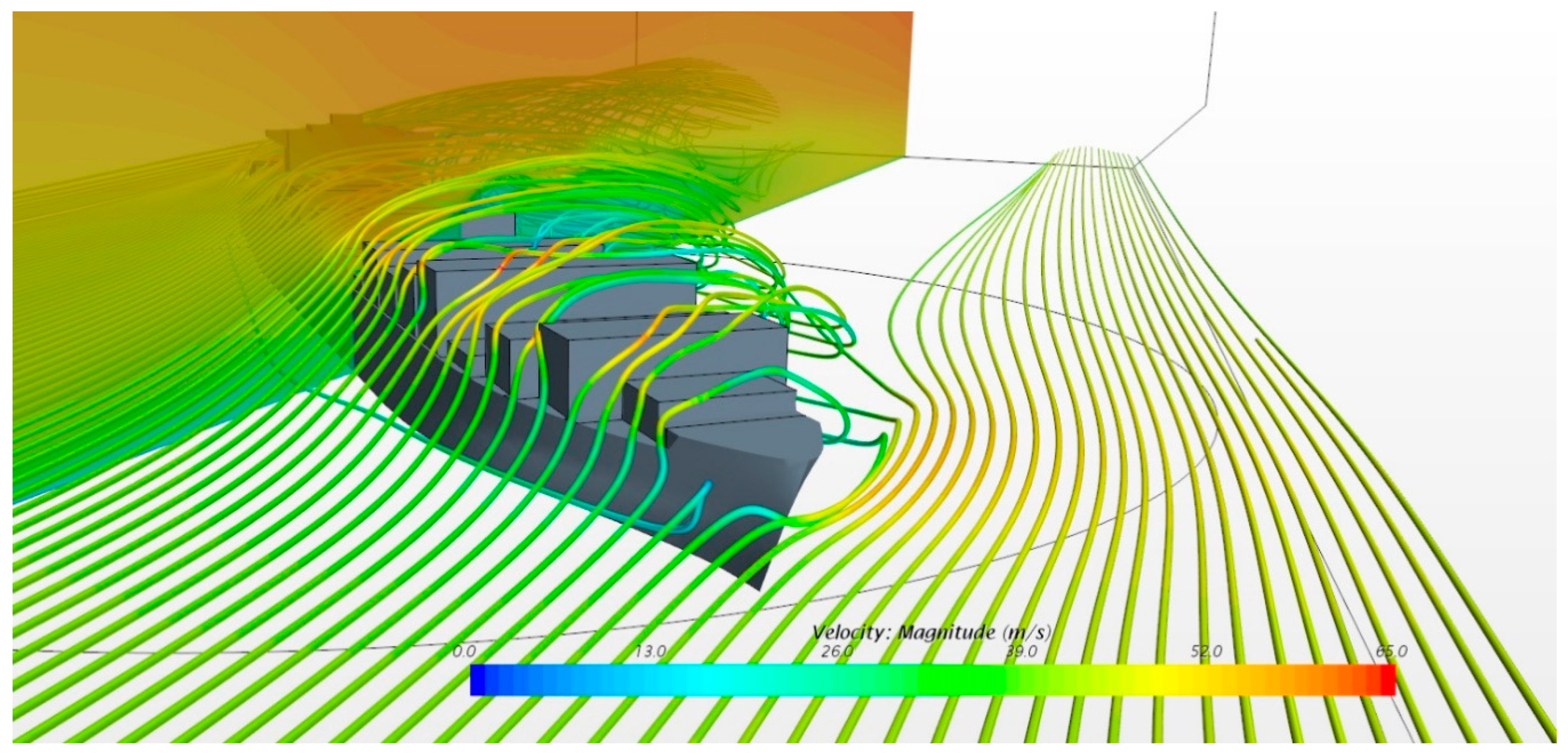
3. Wind Loads Estimation Using CFD

3.1. Computational Geometry and Grid

The computational domain utilized in all the simulations has a rectangular cross-section with chamfered edged so the wind tunnel test section can be adequately replicated. The location of the ships within the domain coincides with the experimental setup described in Anderson [11]. Thirteen different setups of bay configurations have been numerically analyzed using CFD techniques. A demonstrative case, configuration 13 for wind angle 0°, is shown on Figure 5b with trimmed mesh shown on ship surface. Characteristic domain patches are presented in Figure 5a, for configuration 1 case. Remaining patches are fixed walls. The computational domain spans 0.42 m in upstream and 1.44 m in downstream direction, with the cross-section size of 0.6758 m2.
Numerical grids on average contain 3.5 × 10 6 cells. Grids are generated using STAR-CCM+ trim mesher. For all test cases, turbulence in near wall regions is resolved with wall functions.
A typical longitudinal section for configuration 1 is presented in Figure 5c where refinement zones close to ship are clearly visible.

3.2. Boundary Conditions

Wind profile at the inlet has been set in accordance with the Andersen’s specification [11]. Mean velocity as per literature is therefore defined as a function of the domain height:
U ( z ) = U r e f ( z z r e f ) α
where U r e f = 45   m / s is reference velocity, z r e f = 0.0222   m reference height and α = 0.11 velocity profile exponent [23]. Inlet profile of the turbulence dissipation rate ε is determined based on following equation:
ε ( z ) = ( u * ) 3 κ ( z + z 0 )
where κ represents the von Karman constant and u * frictional velocity. Frictional velocity is dependent on the reference velocity and height as per expression:
u * = κ U ( z ) ln ( z r e f + z 0 z 0 )
Aerodynamic roughness length z 0 is estimated based on updated Davenport roughness classification and equals z 0 = 0.0002   m for sea [24,25]. For the model scale this equates to the roughness of z 0 = 4.44 × 10 7   m . Turbulent kinetic energy profile can be estimated and calculated according to:
k ( z ) = ( u * ) 2 C μ .
For z 0.1   m kinetic energy is considered constant so as to avoid any bias since turbulence intensity I U as well as velocity U have not been measured in that range. Employed logarithmic law wall functions ( 30 < y + < 100 ) are modified to account for the roughness based on relationships established by Blocken [25]. These correlations are defined by equation:
k s = 9.793 z 0 C s
where k s represent equivalent sand-grain roughness height and C s roughness constant. In accordance with the aforementioned correlation, equivalent sand-grain roughness has been determined to be k s = 4.35 × 10 6   m with roughness constant equals to C s = 1 . Patches with implemented roughness corrections have been shown in Figure 5a.

3.3. Computational Settings

Navier-Stokes equations describing mechanics of a continuum need to be solved in order to fully resolve fluid flow. These coupled partial differential equations are the result of the Newton’s second law applied to the fluid motion and account for viscosity effects. They are commonly simplified using approximations, with Reynolds-averaged Navier-Stokes (RANS) equations being the most common solution for turbulent flows. To solve these equations, certain assumptions based on experimental data are utilized, thus outlying different RANS turbulent models. Detailed description of RANS models and appropriate closure approaches can be found in Reference [26].
Commercial finite-volume CFD solver Star-CCM+ has been employed to solve aforementioned RANS system of equations with realizable k-ε model ensuring closure of said system. Pressure-velocity coupling is achieved with SIMPLE algorithm. Discretization schemes for all terms are set as second-order. Convergence is assumed when the residuals fall below 10 5 or variance for monitored physical values is less than 0.1% of their mean value.
Figure 6 shows streamlines and central vertical plane colored by velocity magnitude for a single illustrative container configuration and 40-degree ship position rotation from initial position. Complex flow CFD analysis takes into account complete 3D model of a ship above water structure. Included figure demonstrates the complexity of the flow for analyzed cases.

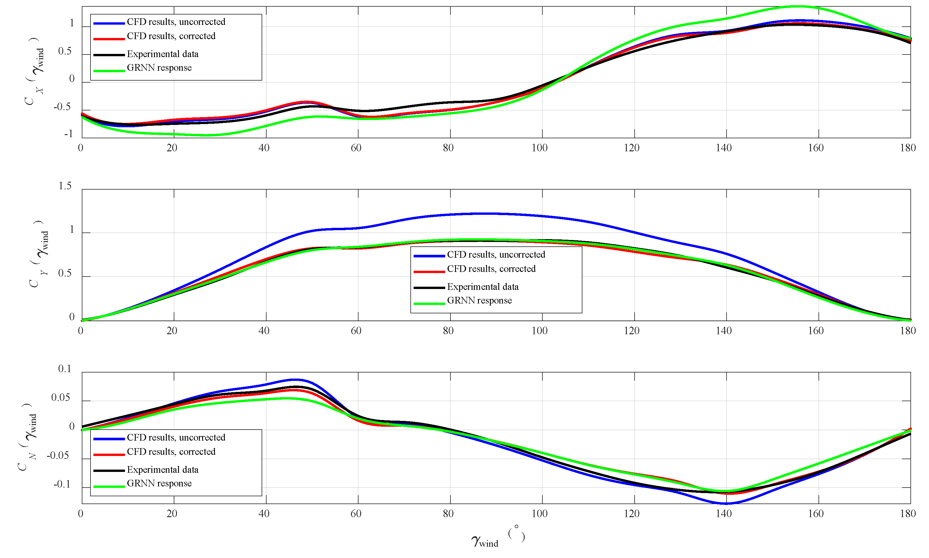
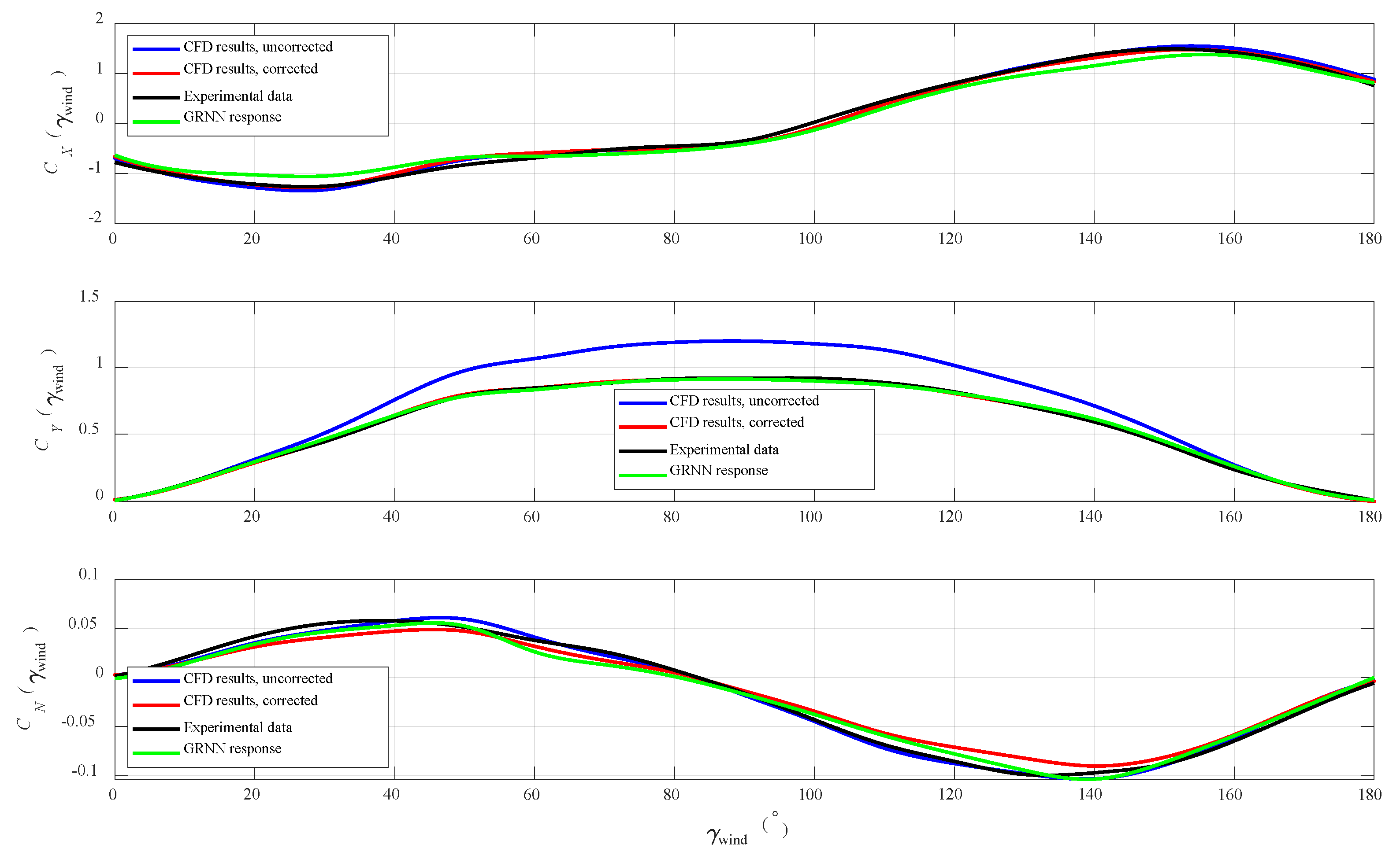
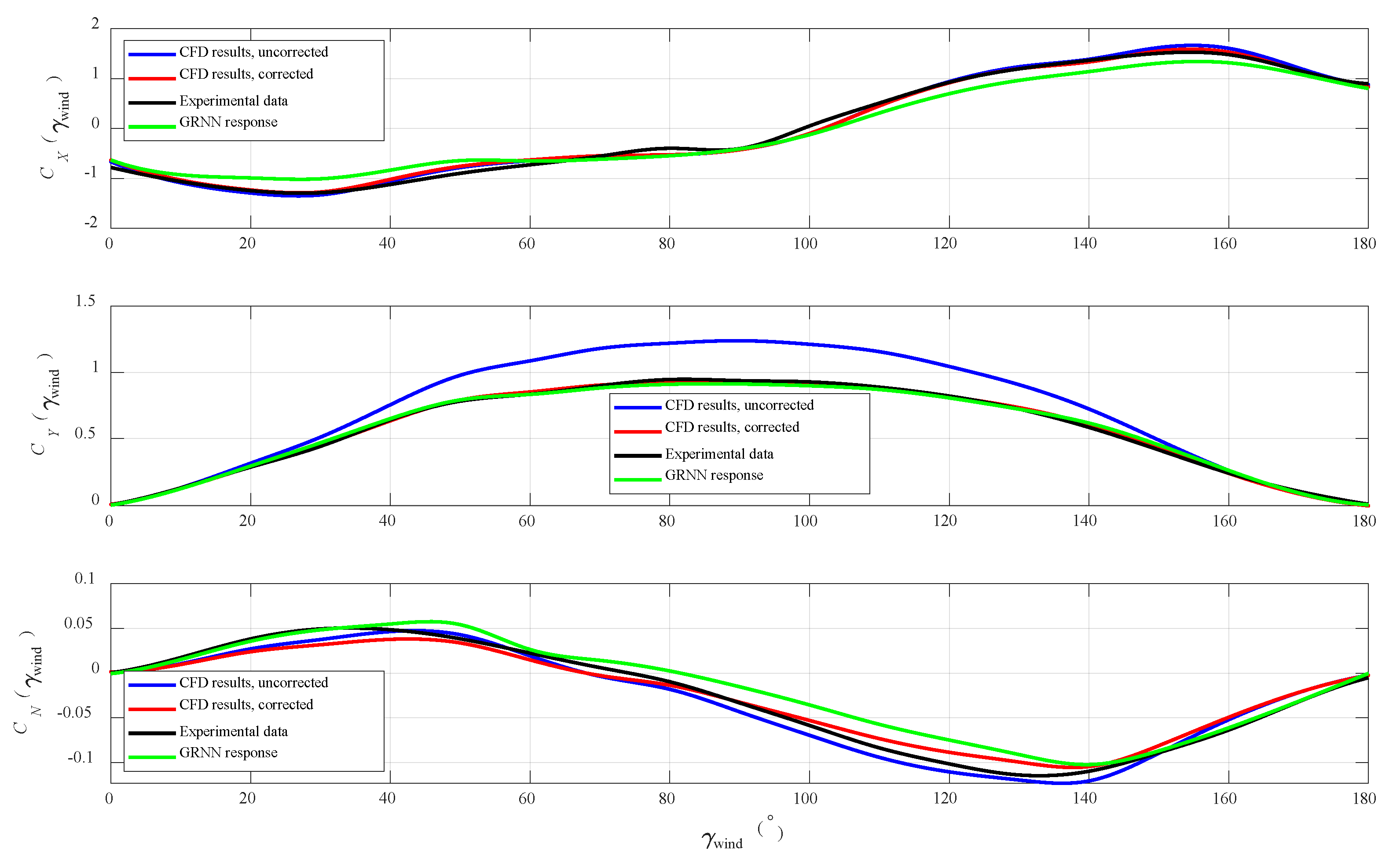
4. Numerical Results

As Andersen [11] carried out an investigation of the influence of container configuration on the deck of a 9000+ TEU container ship on wind forces through a series of wind tunnel tests, the CFD calculation has been run for the same ship. The main characteristics of the ship are: Loa = 340 m, Lpp = 320 m, B = 45 m. Table 1 shows the different container configurations on the deck, which were used for this investigation.
A tunnel wall was added to the CFD simulation’s boundary conditions to ensure similarities with the experimental conditions. So, the calculation has been performed for the two cases: case with no influence of wind tunnel walls (uncorrected, blue line); case with the influence of wind tunnel walls (corrected, red line). In Figure 7, Figure 8, Figure 9, Figure 10, Figure 11, Figure 12, Figure 13, Figure 14, Figure 15, Figure 16, Figure 17, Figure 18 and Figure 19, wind load coefficients CX (γwind), CY (γwind) and CN (γwind), obtained by GRNN (green line) trained with corrected CFD values and Andersen (black line), are compared with the CFD results. The comparison conducted for the i-th vessel is denoted as Conf. #t, t = 1, 2, …, 13.
The results indicate that uncorrected CFD results deviate somewhat from the experimental ones, especially in the transverse direction. However, the corrected values for the case with wind tunnel walls accounted are in line with those obtained experimentally. Those results are in line for the variability of ship lateral contour caused by different container arrangements and indicate good agreement.
The GRNN was trained using input and output set of data for 12 different configurations at a time. The responses are validated for the remaining 13th vessel, as usual in afore mentioned leave-one-out approach. In other words, out of 13 configurations, 12 were used to train the GRNN and then 13th configuration was used for validation. Therefore, when #1 was used for validation, #2 to #13 were used for training. Similarly, when #13 was used for validation, #1 to #12 were used for training.
The wind load coefficients of 13 available container configurations obtained as GRNN responses are compared with corresponding wind load coefficients obtained in wind tunnel testing [11].
Obtained CFD results and GRNN responses can be evaluated in terms of mean values (μi) and associated standard deviations (σi) of absolute differences of appropriate non-dimensional wind load coefficients C i for each degree of freedom in the horizontal plane, i = {X, Y, N} and for each analyzed container configuration t, t = 1, 2, …, 13. However, it does not make sense to compare both of these results directly with available experimental results because GRNNs were trained with the CFD results. Thus, there are two comparisons of interest, that is, comparison A in which CFD results ( C i , t CFD ) are evaluated based on experimental data ( C i , t data ) , and comparison B in which GRNN responses ( C i , t GRNN ) are evaluated with associated CFD results ( C i , t CFD ) , where i = {X, Y, N} and t = 1, 2, …, 13. The results of these comparisons are presented in Table 2.
As expected, based on the obtained values in Table 2, as well as from Figure 7, Figure 8, Figure 9, Figure 10, Figure 11, Figure 12, Figure 13, Figure 14, Figure 15, Figure 16, Figure 17, Figure 18 and Figure 19, it is obvious that GRNN is a slightly less accurate, particularly with some configurations that are somehow unique in comparison to other 12 configurations. That refers particularly to configuration #2, which have almost empty deck and to configuration #7 with alternately arranged empty and full bays.
In addition, it can be noticed that the differences between the experimental data, CFD results (corrected) and GRNN responses are higher for some angles. However, keeping in mind that GRNN training is performed with only 12 configurations at a time, the results clearly indicate that GRNN responses are yet in sufficiently good agreement with wind tunnel experimental values, as well as with corrected CFD results. This particularly stands for lateral coefficients CY that even in this limited set of different container configurations still have sufficient amount of useful and quality information that can be used for GRNN training in terms of EFDs. On the other hand, various longitudinal container configurations lack in terms of quality information, mostly because all these frontal projections are too similar. This justifies larger deviations of GRNN responses of coefficients CX for some container configurations like #3 or #8. These issues are also naturally related to associated yawing coefficients CN.
To conclude, it is reasonable to assume that GRNN accuracy will increase with an increase of available data for new container configurations but also with transition from presented 2D approach, which takes into account only one frontal and one lateral projection, to 3D perspective that should take into account variability of longitudinal cross section projections with variability of lateral projection.

5. Discussion

An enhanced methodology for estimating the wind loads on container ships is presented. Ship frontal and lateral projected areas, that is, their associated closed contours, are represented with elliptic Fourier descriptors. EFDs of closed contours and wind load data derived from CFD analysis are used for GRNN training. As it can be seen in the previous sections, particularly in Chapter 4, very limited number of container configurations were available for conducting this analysis. Therefore, natural choice was to select the so-called leave-one-out cross-validation technique. With this approach, training was performed the number of times that is equal to the number of different container configurations that were analyzed. During this analysis, with each consecutive training, a different container configuration was leaved out for testing, while all other were used for training. The validation of CFD model is based on 13 different container configurations of 9000+ container ship for which the experimental results are provided by Andersen [11]. As indicated, the GRNN was tested on before mentioned 13 different container configurations in a way that the network is trained with the set of data obtained for 12 configurations and the remaining one is used for testing. Taking into account limited input data used for network training, the results show good agreement with the experimental data obtained in wind tunnels.
This approach takes into account all aspects of the variability of the above water frontal and lateral ship profile but with limitation related to the main frontal projection that cannot capture the variability of longitudinal cross sections. However, it is very suitable for the assessment of wind loads on container ships wherever a wind load data for similar ships with various container configurations are available from wind tunnels or are obtained by CFD analysis. In this case, whereas the validity of the CFD analysis has been proven on experimental data, all configurations of interest can be analysed with CFD analysis and larger database can be created. In this way, the cheaper and faster calculation can fill the gap between ship shapes for which calculations or experiments are performed. It is reasonable to assume that the network trained with larger training data set will provide results that are more accurate. Moreover, for the estimation of real wind-induced forces and moment acting on a container ship in open sea-like conditions, the network should be trained with uncorrected values of wind loads coefficients. In other words, the important focus should be put on the initial wind conditions during CFD simulations, because GRNN will be trained with these CFD results and consequently will be trained for some specific wind conditions. Regardless of the conditions under which it was trained, in actual applications of wind loads estimation, trained GRNN requires only simple data such as wind speed and direction, which can be obtained using the wind sensor (anemometer) and areas of frontal and lateral projections that can be easily determined. In other words, it does not require additional wind tunnel testing or CFD simulations, even in a case of completely new configurations that were not used in the training phase. However, if tunnel testing or CFD simulations can be performed and wind load coefficients can be obtained for these “new configurations,” GRNN can be easily and quickly retrained and thus providing higher accuracy and reliability for future estimations.
Further research should be aimed toward uncertainties and reliability analysis, as well to increasing the number of container configurations by means of verified CFD analysis in order to enlarge the available database for neural network training. The selection of neural network type and number of harmonics could also affect the results, so they should be further analyzed as well. The next direction for further research will aim towards the development of a pseudo 3D approach to wind loads estimation on a container ship. This approach will be based on EFDs that are used for ship frontal and lateral closed contour representation of ship cross sections. In this way, all aspects of the 3D variability of the above-water frontal and lateral ship profile will be taken into account.

Author Contributions

Conceptualization, J.P.-O., Z.Č. and M.V.; methodology, J.P.-O., Z.Č. and M.V.; software, Z.Č. and M.V.; validation, J.P.-O., Z.Č. and M.V.; formal analysis, Z.Č. and M.V.; investigation, J.P.-O. and M.V.; resources J.P.-O. and M.V.; data curation, Z.Č. and M.V.; writing, original draft preparation, J.P.-O.; writing, review and editing, J.P.-O., Z.Č. and M.V.; visualization, Z.Č. and M.V.; supervision, J.P.-O.; project administration, J.P.-O. and M.V.; funding acquisition, J.P.-O. All authors have read and agreed to the published version of the manuscript.

Funding

This work was fully supported by the Croatian Science Foundation under the project IP-2018-01-3739. This work was also supported by the University of Rijeka (project no. uniri-tehnic-18-18 1146 and uniri-tehnic-18-266 6469).

Conflicts of Interest

The authors declare no conflict of interest.

Abbreviations

The following abbreviations are used in this manuscript:
CADComputer-Aided Design
CFDComputational Fluid Dynamics
EFDElliptic Fourier Descriptors
GRNNGeneralized Regression Neural Network
LNGLiquefied Natural Gas
NEDNorth-East-Down
NNNeural Network
RANSReynolds-averaged Navier–Stokes

References

  1. Isherwood, R.M. Wind resistance of merchant ships. R. Inst. Nav. Archit. 1972, 114, 327–338. [Google Scholar]
  2. Gould, R.W.F. The Estimation of Wind Loads on Ship Superstructures; Monograph, No. 8; The Royal Institution of Naval Architects: London, UK, 1982; p. 34. [Google Scholar]
  3. Blendermann, W. Schiffsform und Windlast-Korrelations-und Regressionanalyse von Windkanalmes-Sungen am Modell; Report No. 533; Institut fur Schiffbau der Universitat Hamburg: Hamburg, Germany, 1993; 132p. [Google Scholar]
  4. Blendermann, W. Parameter identification of wind loads on ships. J. Wind Eng. Ind. Aerodyn. 1994, 51, 339–351. [Google Scholar] [CrossRef]
  5. Blendermann, W. Estimation of wind loads on ships in wind with a strong gradient. In Proceedings of the 14th International Conference on Offshore Mechanics and Arctic Engineering (OMAE), New York, NY, USA, 18–22 June 1995; ASME: New York, NY, USA, 1995; Volume l-A, pp. 271–277. [Google Scholar]
  6. Blendermann, W. Floating docks: Prediction of wind loads in extreme winds. Schiff Hafen 1996, 48, 67–70. [Google Scholar]
  7. Haddara, M.R.; Guedes Soares, C. Wind loads on marine structures. Mar. Struct. 1999, 12, 199–209. [Google Scholar] [CrossRef]
  8. Brizzolara, S.; Rizzuto, E. Wind heeling moments on very large ships. Some insights through CFD results. In Proceedings of the 9th International Conference on Stability of Ships and Ocean Vehicles, Rio de Janeiro, Brazil, 25–29 September 2006; pp. 781–793. [Google Scholar]
  9. Wnek, A.D.; Guedes Soares, C. CFD assessment of the wind loads on an LNG carrier and floating platform models. Ocean. Eng. 2015, 97, 30–36. [Google Scholar] [CrossRef]
  10. Janssen, W.D.; Blocken, B.; van Wijhe, H.J. CFD simulations of wind loads on a container ship: Validation and impact of geometrical simplifications. J. Wind. Eng. Ind. Aerodyn. 2017, 166, 106–116. [Google Scholar] [CrossRef] [Green Version]
  11. Andersen, I.M.V. Wind loads on post-panamax containership. Ocean Eng. 2013, 58, 115–134. [Google Scholar] [CrossRef]
  12. Valčić, M.; Prpić-Oršić, J. Hybrid method for estimating wind loads on ships based on elliptic Fourier analysis and radial basis neural networks. Ocean Eng. 2016, 122, 227–240. [Google Scholar] [CrossRef]
  13. Prpić-Oršić, J.; Valčić, M.; Vučinić, D. Application of pattern recognition method for estimating wind loads on ships and marine objects. In Materialwissenschaft und Werkstofftechnik—Material Science and Engineering Technology; WILEY-VCH Verlag GmbH & Co. KGaA: Weinheim, Germany, 2017; Volume 48, pp. 387–400. [Google Scholar]
  14. Valčić, M.; Prpić-Oršić, J.; Vučinić, D. Application of pattern recognition method for estimating wind loads on ships and marine objects. In Visual Computing—Advancing Engineering Practice; Series Lecture Notes in Mechanical Engineering; Springer: Singapore, 2019; 38p. [Google Scholar]
  15. Prpić-Oršić, J.; Valčić, M. Sensitivity analysis of wind load estimation method based on elliptic Fourier descriptors. In Proceedings of the Maritime Technology and Engineering—MARTECH 2016, Lisabon, Portugal, 4–6 July 2016; pp. 151–160. [Google Scholar]
  16. Specht, D.F. A General Regression Neural Network. IEEE Trans. Neural Netw. 1991, 2, 568–576. [Google Scholar] [CrossRef] [PubMed] [Green Version]
  17. Freeman, H. Computer Processing of Line-Drawing Images. Comput. Surv. 1974, 6, 57–97. [Google Scholar] [CrossRef]
  18. Granlund, G.H. Fourier Preprocessing for Hand Print Character Recognition. IEEE Trans. Comput. 1972, 21, 195–201. [Google Scholar] [CrossRef]
  19. Pavlidis, T. Algorithms for Graphics and Image Processing; Springer: Berlin/Heidelberg, Germany, 1982. [Google Scholar]
  20. Nixon, M.S.; Aguado, A.S. Feature Extraction and Image Processing, 2nd ed.; Academic Press (Elsevier): London, UK, 2008. [Google Scholar]
  21. Kuhl, F.P.; Giardina, C.R. Elliptic Fourier Features of a Closed Contour. Comput. Graph. Image Process. 1982, 18, 236–258. [Google Scholar] [CrossRef]
  22. Fossen, T.I. Handbook of Marine Craft Hydrodynamics and Motion Control; John Wiley & Sons Ltd.: Chichester, UK, 2011. [Google Scholar]
  23. Norwegian Maritime Directory. Regulations for Mobile Offshore Units. 1997. Available online: http://www.sjofartsdir.no/en/Legislation_and_International_Relations/Translated_Norwegian_legislation/Regulations-for-Mobile-Offshore-Units (accessed on 20 June 2020).
  24. Wieringa, J. Updating the Davenport roughness classification. J. Wind Eng. Ind. Aerodyn. 1992, 41, 357–368. [Google Scholar] [CrossRef]
  25. Blocken, B.; Carmeliet, J.; Stathopoulos, T. CFD evaluation of the wind speed conditions in passages between buildings—Effect of wall-function roughness modifications on the atmospheric boundary layer flow. J. Wind Eng. Ind. Aerodyn. 2007, 95, 941–962. [Google Scholar] [CrossRef]
  26. Ferziger, J.H.; Peric, M. Computational Methods for Fluid Dynamics; Springer Science & Business Media: Berlin/Heidelberg, Germany, 2012. [Google Scholar]
Figure 1. Reference frames and notation.
Jmse 08 00539 g001
Figure 2. Enhanced methodological framework for wind load estimation based on Computational Fluid Dynamics CFD, Elliptic Fourier Descriptors (EFDs) and Generalized Regression Neural Network (GRNN).
Jmse 08 00539 g002
Figure 3. Vector representation and visualization of Freeman chain encoding with contour extraction.
Jmse 08 00539 g003
Figure 4. Fitting of the closed contour with different number of harmonics N.
Jmse 08 00539 g004aJmse 08 00539 g004b
Figure 5. Computational domain (a), computational grid on the ship surface (b) for different bay loading of configuration #1 (c).
Jmse 08 00539 g005
Figure 6. Streamlines and central vertical plane colored by velocity magnitude.
Jmse 08 00539 g006
Figure 7. Wind loads coefficients for configuration #1.
Jmse 08 00539 g007
Figure 8. Wind loads coefficients for configuration #2.
Jmse 08 00539 g008
Figure 9. Wind loads coefficients for configuration #3.
Jmse 08 00539 g009
Figure 10. Wind loads coefficients for configuration #4.
Jmse 08 00539 g010
Figure 11. Wind loads coefficients for configuration #5.
Jmse 08 00539 g011
Figure 12. Wind loads coefficients for configuration #6.
Jmse 08 00539 g012
Figure 13. Wind loads coefficients for configuration #7.
Jmse 08 00539 g013
Figure 14. Wind loads coefficients for configuration #8.
Jmse 08 00539 g014
Figure 15. Wind loads coefficients for configuration #9.
Jmse 08 00539 g015
Figure 16. Wind loads coefficients for configuration #10.
Jmse 08 00539 g016
Figure 17. Wind loads coefficients for configuration #11.
Jmse 08 00539 g017
Figure 18. Wind loads coefficients for configuration #12.
Jmse 08 00539 g018
Figure 19. Wind loads coefficients for configuration #13.
Jmse 08 00539 g019
Table 1. Analyzed containership configurations [11].
#Frontal Configu-RationLateral Configuration#Frontal Configu-RationLateral Configuration
1 Jmse 08 00539 i001 Jmse 08 00539 i0028 Jmse 08 00539 i003 Jmse 08 00539 i004
2 Jmse 08 00539 i005 Jmse 08 00539 i0069 Jmse 08 00539 i007 Jmse 08 00539 i008
3 Jmse 08 00539 i009 Jmse 08 00539 i01010 Jmse 08 00539 i011 Jmse 08 00539 i012
4 Jmse 08 00539 i013 Jmse 08 00539 i01411 Jmse 08 00539 i015 Jmse 08 00539 i016
5 Jmse 08 00539 i017 Jmse 08 00539 i01812 Jmse 08 00539 i019 Jmse 08 00539 i020
6 Jmse 08 00539 i021 Jmse 08 00539 i02213 Jmse 08 00539 i023 Jmse 08 00539 i024
7 Jmse 08 00539 i025 Jmse 08 00539 i026
Table 2. Comparison of obtained results in terms of mean values (μi) and standard deviations (σi) of absolute differences of wind load coefficients in cases A (CFD vs. data) and B (GRNN vs. CFD).
A: CFD Results vs. Experimental DataB: GRRN Responses vs. CFD Results
t μ X ( C X , t CFD C X , t data )
σ X ( C X , t CFD C X , t data )
μ Y ( C Y , t CFD C Y , t data )
σ Y ( C Y , t CFD C Y , t data )
μ N ( C N , t CFD C N , t data )
σ N ( C N , t CFD C N , t data )
μ X ( C X , t GRNN C X , t CFD )
σ X ( C X , t GRNN C X , t CFD )
μ Y ( C Y , t GRNN C Y , t CFD )
σ Y ( C Y , t GRNN C Y , t CFD )
μ N ( C N , t GRNN C N , t CFD )
σ N ( C N , t GRNN C N , t CFD )
10.006830
0.077113
0.000001
0.022939
0.001013
0.007878
−0.018669
0.083724
−0.013219
0.008449
0.001119
0.004969
20.028897
0.070867
−0.031025
0.029837
0.000250
0.006619
0.019692
0.156943
0.036904
0.021176
0.005489
0.006890
3−0.001519
0.067631
−0.002002
0.016848
0.001721
0.007465
0.021038
0.217758
−0.005834
0.007852
−0.003374
0.008509
4−0.040542
0.069472
−0.001895
0.024665
0.001351
0.008477
0.039521
0.126639
−0.001958
0.011143
−0.005018
0.004919
5−0.027537
0.071166
0.000302
0.021155
0.000559
0.008445
0.066050
0.124721
−0.003438
0.013194
−0.011163
0.009887
60.004378
0.066045
0.000507
0.021938
0.000101
0.007114
−0.011767
0.190404
−0.001516
0.020347
−0.000170
0.007039
70.009061
0.079468
−0.009399
0.028647
0.002226
0.007970
−0.095680
0.076000
−0.013755
0.017702
0.013060
0.009611
80.015437
0.112929
−0.004332
0.014446
0.001051
0.016156
−0.032795
0.642980
0.008992
0.020995
0.009923
0.017630
9−0.000038
0.061642
−0.000605
0.010249
0.001022
0.008962
−0.020133
0.106340
0.001654
0.008042
−0.002510
0.005232
100.006541
0.072194
−0.000360
0.012062
0.000443
0.009953
−0.028850
0.157382
−0.001015
0.014933
0.008996
0.009849
110.008620
0.090098
−0.021369
0.014297
0.000902
0.006874
0.020806
0.128550
0.009962
0.006351
−0.004635
0.005230
12−0.012284
0.079605
−0.015912
0.020094
0.000107
0.007031
0.042008
0.231174
0.003056
0.007483
−0.002915
0.008500
130.025503
0.103171
−0.026480
0.019025
0.001303
0.007147
0.035129
0.163835
0.008007
0.006242
−0.006211
0.007112

