Large Eddy Simulation of Microbubble Drag Reduction in Fully Developed Turbulent Boundary Layers

Abstract

Microbubble drag reduction has good application prospects. It operates by injecting a large number of bubbles with tiny diameters into a turbulent boundary layer. However, its mechanism is not yet fully understood. In this paper, the mechanisms of microbubble drag reduction in a fully developed turbulent boundary layer over a flat-plate is investigated using a two-way coupled Euler-Lagrange approach based on large eddy simulation. The results show good agreement with theoretical values in the velocity distribution and the distribution of fluctuation intensities. As the results show, the presence of bubbles reduces the frequency of bursts associated with the sweep events from 637.8 Hz to 611.2 Hz, indicating that the sweep events, namely the impacting of high-speed fluids on the wall surface, are suppressed and the streamwise velocity near the wall is decreased, hence reducing the velocity gradient at the wall and consequently lessening the skin friction. The suppression on burst frequency also, with the fluid fluctuation reduced in degree, decreases the intensity of vortices near the wall, leading to reduced production of turbulent kinetic energy.

1. Introduction

In microbubble drag reduction (MDR), a large number of microbubbles are introduced into a turbulent boundary layer (TBL) to form a mixed layer of gas and liquid. Due to its large rate of drag reduction and wide range of applicability, it is considered the most promising method of drag reduction in the shipping sector [1,2,3,4,5,6]. A clear understanding of the mechanism of MDR can promote better application of this technology, helping to conserve energy and promote sustainable development. However, unlike the use of layers of air, or super-cavities, which reduce drag by insulating the object from contact with water [7], the mechanism of MDR is more complex because the bubbles do not directly come into contact with the wall of the object, simply appearing in the turbulent boundary layers. Therefore, it is generally believed that the presence of microbubbles changes the structure of the boundary layer [8]. The excellent prospects for application and complex mechanism of drag reduction in microbubbles have attracted researchers’ attention to their use, which has made it a research hotspot in recent years.

The study of MDR can be divided into the study of apparent laws and microscopic mechanisms. Research into the apparent laws of this phenomenon began in the 1970s and was largely experimental. McCormick and Bhattacharyya [9] examined MDR for an axisymmetric body in a towing tank. They used electrolysis to generate the bubbles and found that their presence greatly reduced frictional drag. The greater the current, the better the effect, and the maximum drag reduction effect reached 50%. Madavan [10] performed a drag reduction experiment on a plate in a cavitation tunnel. He used microporous plates to generate microbubbles and found that the drag is proportional to the velocity of inflow and inversely proportional to the velocity of ventilation. The maximum drag reduction achieved reached 85%. These studies confirmed the existence of MDR. Subsequently, research began to focus on the influence of the parameters of flow fields on the effect. Merkle and Deutsch [11] studied the effects of size and amount of pore on drag reduction. They used a porous plate with pore sizes from 1 µm to 50 µm to generate microbubbles and found that the smaller the diameter of the pore, the greater the drag reduction, and it was greatest when the diameter was 1–3 µm. The volume concentration of the bubble reached a maximum at a thickness of 1/10 of the boundary layer of the wall. Kawamura [12] studied the effects of different bubble diameters on drag reduction and found for bubble diameters in the range of 0.5–2 mm, changes in diameter had little effect on the rate of drag reduction. However, for bubble diameters on the order of 10 µm, drag was effectively reduced. Shen [13] injected bubbles of different diameters into clean water and brine to study the effects of bubble diameters and fluid media on drag reduction. He used three diameters, of 476, 322, and 254 µm, and found that changes in diameter had little effect on drag reduction, with almost no difference in drag reduction between clear water and brine. Fontaine and Deutsch [14] studied the effects of different gases on drag reduction. They chose several gases with different densities and solubilities and set a large range of variation. They found that the type of gas had little effect on drag reduction. In recent years, the Reynolds-averaged Navier-Stokes (RANS) has also been used as an auxiliary method. Zhao [15] studied the drag reduction produced by microbubbles on an axisymmetric body using a standard k–ε model and a Eulerian–Eulerian two-fluid model to reproduce some of the laws found in experimental research. Song [16] investigated the effects of microbubble drag reduction on an axisymmetric body, including the injection position and bubble parameters.

The study of microscopic mechanisms of MDR generally uses Direct Numerical Simulation (DNS) and Large Eddy Simulation (LES), because such studies require enough information on turbulence which RANS cannot provide. Some studies have also used theoretical analysis. Bogdevich [17] performed a plate drag reduction experiment in a cavitation tunnel. He used microporous plates to generate microbubbles and found for the first time that the injected microbubbles caused a significant change in the boundary layer structure. Legner [18] proposed a stress model to explain the mechanism of drag reduction in microbubbles. He found that drag reduction was a combined effect, caused by density reduction and changes in turbulence characteristics. When the bubble volume reaches the containment limit, the maximum amount of drag reduction is attained. The rapid increase in the viscosity of the medium is an obstacle to further drag reduction. Madavan [19] had a similar conclusion, namely, that the drag reduction effect was greatest when the bubble remained in the transition layer of the turbulent boundary layer. Kanai and Miyata [20] used a density function to directly simulate the flow of bubbles in a pipeline under turbulent flow conditions. The interactions between the bubbles and wall turbulence was discussed, and the drag reduction of the turbulent boundary layer containing microbubbles was characterized. Ferrante and Elghobashi [8] used the Euler–Lagrange method to directly simulate the spatially developed turbulent boundary layer containing microbubbles. It was found that, after the injection of the microbubbles, due to the gradient of the bubble volume, a velocity component perpendicular to the wall surface and pointing upward was induced; this component pushed the quasi-streamwise vortex structure away from the wall, causing the impact of the sweeping fluid on the wall to weaken. The flow velocity of the wall was reduced, resulting in a decrease in drag. Ferrante and Elghobashi [21] then performed a series of numerical simulations of different Reynolds numbers and found that after the Reynolds number was increased, the drag reduction rate decreased. In recent years, Zhang [22] investigated the bubble-turbulence interaction in turbulent channel flow and boundary layer flow with a two-way coupled Euler–Lagrange code. The corresponding drag reduction effect was studied. To accurately simulate the bubble–wall interaction, they treated immersed bubbles with a nonlinear collision model and valuable results were achieved.

There are two fields related to microbubbles which are necessarily listed here to provide a whole picture and ideas for further study of MDR. The first is the transition from MDR to air-layer drag reduction. Elbing [23,24] conducted experiments to study this phenomenon. The critical volumetric flux of air required to achieve an air layer was observed to be approximately proportional to the square of the free-stream speed. Yu [25] conducted a series of valuable studies to reveal the mechanisms of air-layer drag reduction and found that when the air layer was formed, the density, viscosity, and velocity gradients at the bottom of the boundary layer were reduced, which led to a decrease in drag. Ceccio [26] provided a detailed review of this topic. The second is the bubbles in cloud cavitation experiencing breakups and coalescence under the interactions with turbulence structure. Du [27] proposed a numerical model that can resolve the distribution of the density of the number of bubbles and can be used to elucidate the internal structures of cloud cavitation. Long [28] studied the interactions between cavitation and turbulence structures using LES and the Euler–Lagrange method and found that once the cavity was cut off, the evolution of the vortex structure significantly affected local cavitating flow. These findings can help us to understand the bubble behavior under turbulence.

In this study, the microscopic mechanisms of MDR are examined in a fully developed turbulent boundary layer over a flat-plate. The content includes: (i) the discussion of the movement of microbubbles under the interaction with turbulence structure; (ii) the analyzing of the mechanisms of MDR with the investigation on bursts and velocity gradient; and (iii) the examining of vortex intensity and turbulent kinetic energy.

2. Numerical Methodology

2.1. Basic Governing Equations

The basic principle of LES is spatial filtering of the Navier–Stokes equations. It filters small-scale turbulence out of the equations and directly calculates large-scale turbulence. The scale of filtering is referred to as the subgrid scale. Because the turbulence below this scale is similar, it is feasible to use a subgrid model to close the equations. This only requires the calculation of large-scale turbulence, which greatly reduces the amount of calculation needed. The calculations in this paper used the CFX module in ANSYS 17.1 and used 64 cores of AMD Opteron 6276 and 128G Memory. The basic governing equations for fluid dynamics are as follows:

$$\frac{\partial \rho }{\partial t}+\frac{\partial \left(\rho u_i\right)}{x_i}=0$$

(1)

$$\frac{\partial \left(\rho u_i\right)}{\partial t}+\frac{\partial \left(\rho u_i{u}_j\right)}{\partial x_j}=-\frac{\partial p}{\partial x_i}+\frac{\partial {\tau }_{ij}}{\partial x_j}+S_M$$

(2)

Here, formula (1) is the continuity equation, and formula (2) is the momentum equation. Because the calculations in this paper do not involve heat transfer, the energy equation is not described. The $\rho$ is fluid density, p is pressure, $x_i$ is the Cartesian coordinate, $u_i$ is the velocity component in the Cartesian coordinates (i = 1, 2, 3), and $S_M$ is the volume force or other added source term. The expression of the shear stress ${\tau }_{ij}$ is as follows:

$${\tau }_{ij}=\mu \left(\frac{\partial u_i}{\partial x_j}+\frac{\partial u_j}{\partial x_i}-\frac{2}{3}{\delta }_{ij}\frac{\partial u_k}{\partial x_k}\right)$$

(3)

where µ is the viscosity of the fluid, and ${\delta }_{ij}$ is the Kronecker symbol. The filter function is recorded as $G\left(x;x^{\prime }\right)$. Then the filtering of any turbulence is equal to:

$$\overline{f}\left(x\right)={\displaystyle \int }f\left(x^{\prime }\right)G\left(x;x^{\prime }\right)d{x}^{\prime }$$

(4)

The filter function uses a box filter, and its equation is as follows:

$$G\left(\left|x-x^{\prime }\right|\right)=\{\begin{array}{c}\frac{1}{\Delta x_1\Delta x_2\Delta x_3}\hspace{1em}\left|x_i^{\prime }-x_i\right|\le \frac{\Delta x_i}{2}i=1,2,3\\ 0\hspace{1em}\hspace{1em}\hspace{1em}\left|x_i^{\prime }-x_i\right|>\frac{\Delta x_i}{2}i=1,2,3\end{array}$$

(5)

For incompressible fluids, the basic equations after filtering are:

$$\frac{\partial \overline{u_i}}{\partial x_i}=0$$

(6)

$$\frac{\partial \left(\rho \overline{u_i}\right)}{\partial t}+\frac{\partial }{\partial x_j}\left(\rho \overline{u_i}\overline{u_j}\right)=-\frac{\partial \overline{p}}{\partial x_i}+\frac{\partial }{\partial x_j}\left[\mu \left(\frac{\partial \overline{u_i}}{\partial x_j}+\frac{\partial \overline{u_j}}{\partial x_i}\right)\right]+\frac{\partial {\sigma }_{ij}}{\partial x_j}$$

(7)

where Equation (6) is the continuity equation, and Equation (7) is the momentum equation. A new unknown ${\sigma }_{ij}$ appears in the filtered equation. ${\sigma }_{ij}$ is the subgrid stress, which represents the effect of filtered small-scale turbulence on a large scale. This expression is:

$${\sigma }_{ij}=-\overline{\rho u_i{u}_j}+\overline{\rho }\overline{u_i}\overline{u_j}$$

(8)

An eddy viscosity method was introduced to relate the subgrid stress ${\sigma }_{ij}$ to the large-scale shear strain tensor ${\overline{S}}_{ij}$. The expression is as follows:

$${\sigma }_{ij}-\frac{1}{3}{\delta }_{ij}{\sigma }_{kk}=2{\mu }_{sgs}{\overline{S}}_{ij}$$

(9)

$${\overline{S}}_{ij}=\frac{1}{2}\left(\frac{\partial u_i}{\partial x_j}+\frac{\partial u_j}{\partial x_i}\right)$$

(10)

where ${\sigma }_{kk}$ is given directly by static pressure after filtration. In the equation, only ${\mu }_{sgs}$ is an unknown quantity, and ${\mu }_{sgs}$ is given by the subgrid model; in this paper, this is the WALE model [29], which is a wall-adapted model of local eddy viscosity. The expression is as follows:

$${\mu }_{sgs}=\rho {\left(C_W\Delta \right)}^2\frac{{\left(S_{ij}^d{S}_{ij}^d\right)}^{3/2}}{{\left({\overline{S}}_{ij}{\overline{S}}_{ij}\right)}^{5/2}+{\left(S_{ij}^d{S}_{ij}^d\right)}^{5/4}}$$

(11)

where

$$S_{ij}^d=\frac{1}{2}\left({\overline{g}}_{ij}^2+{\overline{g}}_{ji}^2\right)-\frac{1}{3}{\delta }_{ij}{\overline{g}}_{kk}^2$$

(12)

$${\overline{g}}_{ij}^2={\overline{g}}_{ik}{\overline{g}}_{kj}$$

(13)

$${\overline{g}}_{ij}=\frac{\partial {\overline{u}}_i}{\partial x_j}$$

(14)

$C_W$ is a constant with a value of 0.5. The advantage of the WALE model is that it can make a transition from laminar to turbulent. It has the same advantages as the dynamic Smagorinsky–Lilly model [30,31], and it does not require secondary filtering.

2.2. Euler–Lagrange Model

The Euler–Lagrange model is one of the most commonly used methods in the numerical simulation of microbubbles [32,33,34,35]. If the time step is small enough, the movement of a particle is considered uniform in that step. Using ${\mathit{x}}_p$ to represent the position vector of a particle, after a time step, the position of the particle changes to the following:

$${\mathit{x}}_p^{n+1}={\mathit{x}}_p^n+{\mathit{U}}_p^n\Delta t$$

(15)

where ${\mathit{U}}_p$ is the particle velocity vector. The velocity vector is solved by Newton’s second law, as shown below:

$$m_p\frac{d{\mathit{U}}_p}{dt}={\mathit{F}}_D+{\mathit{F}}_G+{\mathit{F}}_B+{\mathit{F}}_{VM}$$

(16)

where ${\mathit{F}}_D$ is the drag force, ${\mathit{F}}_G$ is the gravity, ${\mathit{F}}_B$ is the buoyancy, and ${\mathit{F}}_{VM}$ is the virtual mass force. It should be noted that the force on the particles goes beyond the three forces noted here, as they are affected by the centripetal force and the Coriolis force in a rotating fluid. However, in this context, those forces are negligible and are not discussed.

Following the Euler-Lagrange method, the force of a continuous relative particle is applied directly to the particle, and the force of the particle in the continuous phase is transmitted through a source term for momentum. Equation (17) is the drag force, and Equation (19) is the virtual mass force:

$${\mathit{F}}_D=\frac{1}{2}{C}_D{\rho }_{c}A\left|{\mathit{U}}_c-{\mathit{U}}_p\right|\left({\mathit{U}}_c-{\mathit{U}}_p\right)$$

(17)

$$C_D=\max \left(\frac{24}{\mathrm{Re}}\left(1+0.15{\mathrm{Re}}^{0.687}\right),0.44\right)$$

(18)

$${\mathit{F}}_{VM}=\frac{C_{VM}}{12}\pi d_p^3{\rho }_c\left(\frac{d{\mathit{U}}_c}{dt}-\frac{d{\mathit{U}}_p}{dt}\right)$$

(19)

where $C_D$ is the drag coefficient, $C_{VM}$ is the virtual mass coefficient, ${\rho }_c$ is the continuous phase density, $A$ is the effective cross-sectional area of particle, and ${\mathit{U}}_c$ and ${\mathit{U}}_p$ are velocity vectors for the continuous phase and particles. In the simulation, $C_{VM}$ has the value of 0.5 obtained from the inviscid flow around an isolated sphere. The momentum source terms for drag force and virtual mass force are calculated using the following equations:

$$\frac{d{\mathit{S}}_D}{dt}=-{\mathit{F}}_D$$

(20)

$$\frac{d{\mathit{S}}_{VM}}{dt}=-{\mathit{F}}_{VM}$$

(21)

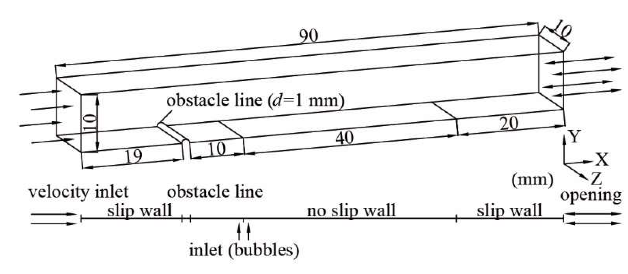
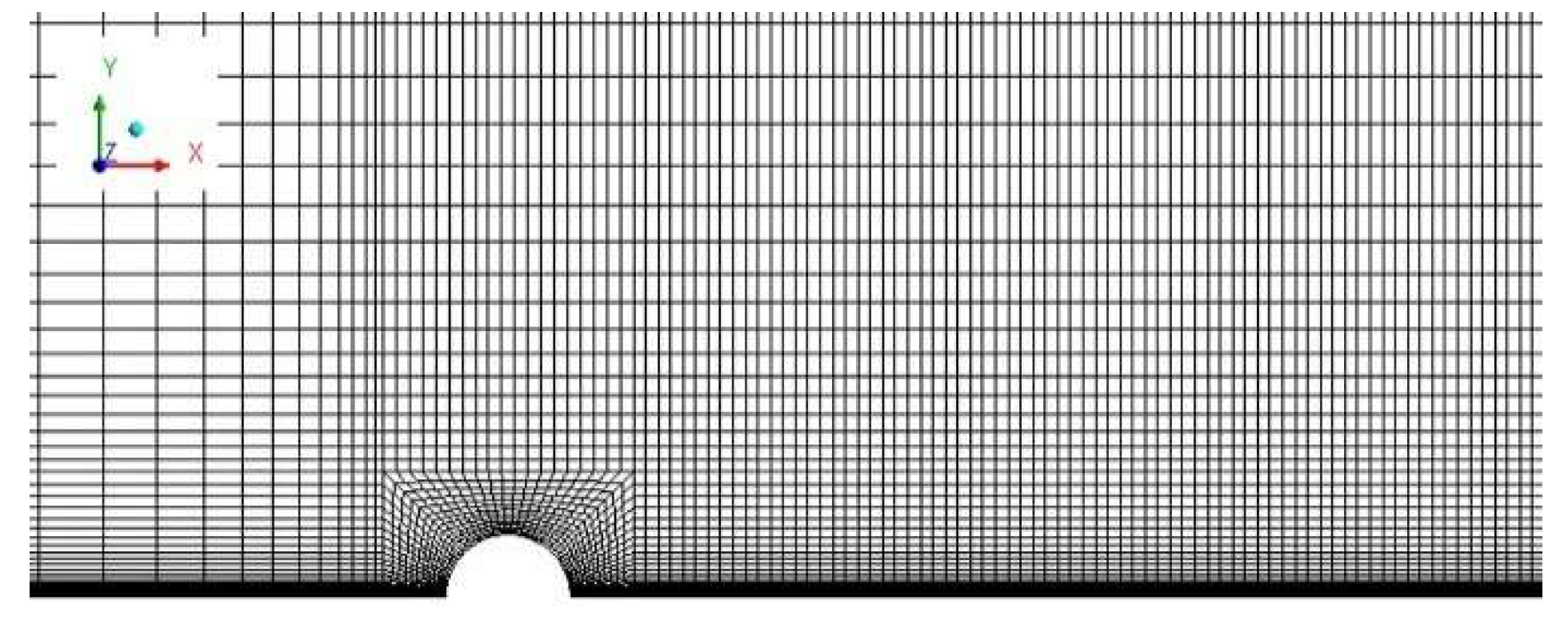
2.3. Computational Domain and Boundary Conditions

The parameters for mesh and simulation are determined based on the following two constraints. On the one hand, it is necessary to ensure that there are enough turbulence structures, including streaks and streamwise vortices, in the calculation domain to meet the research requirements. The size of a streak can be estimated by the average length of $1000–2000\nu /u_{\tau }$, the average height of $10–25\nu /u_{\tau }$, and the average span spacing of $100\nu /u_{\tau }$. The size of a streamwise vortex can be estimated by the average length of $40\nu /u_{\tau }$, and the average vertical height of $15–20\nu /u_{\tau }$, where $\mathsf{\nu }$ is the kinematic viscosity and $u_{\tau }$ is the wall friction velocity [36]. On the other hand, LES requires $\Delta y^{+}<1$, $\Delta x^{+}\approx 30$ and $\Delta z^{+}\approx 15$ for the mesh and a courant number less than 0.5 [37].

The above requirements and reference settings [8] indicate that the dimensions of the calculation domain are 90 mm streamwise, 10 mm in the normal direction, and 10 mm spanwise. To eliminate the influence of the inlet on downstream phenomena, a 19 mm inlet section and a 20 mm outlet section were set up in the same way. The diameter of the obstacle line was 1 mm, and the length of the flat-plate was 50 mm, as shown in Figure 1. In this paper, the streamwise dimension is x, the normal is y, and the spanwise dimension is z. A mesh of $\Delta y^{+}=0.7$, $\Delta x^{+}=37$ and $\Delta z^{+}=18$ is generated and it is evenly distributed in the streamwise and spanwise and is densified in the near-wall area in the normal direction. The amount of global mesh is 6.88 million. A magnified view of the area near the obstacle line is shown in Figure 2.

The simulation parameters are determined as shown in

Table 1. Flow field and bubble properties.

Case	Timestep (s)	${\mathit{U}}_{\infty }(\mathbf{m}/\mathbf{s})$	${\mathit{U}}_{\mathit{b}}(\mathbf{m}/\mathbf{s})$	${\mathit{d}}_{\mathit{b}}(\mathsf{\mu }\mathbf{m})$	${\mathit{N}}_{\mathit{b}}\left({\mathbf{s}}^{-1}\right)$	${\mathit{u}}_{\mathit{\tau }}(\mathbf{m}/\mathbf{s})$
A	$1\times {10}^{-6}$	7	0.2	40	$5\times {10}^6$	0.3286
B	$1\times {10}^{-6}$	7	2	40	$5\times {10}^6$	0.3381

, $U_{\infty }$ is the inflow velocity, and $U_b$ is the velocity at which bubbles are injected into the flow field. The velocity direction of $U_b$ is perpendicular to the wall surface. The inflow velocity was set to 7 m/s and time step was $1\times {10}^{-6}$ s to meet the requirements for courant number and dimensionless mesh size, as well as the requirement for velocity to generate a fully developed turbulent boundary layer. The bubble velocity has two different values to compare the rates of drag reduction at different $U_b$. The distribution of bubble diameters in this paper is a normal distribution, with a standard deviation of 1 µm and an average diameter of $d_b$, due to the experiment results conducted by Song [16]. The $d_b$ is set to 40 µm to achieve the best effects according to prior research [11,13], which has confirmed that microbubble diameters below 50 µm can achieve the best effects. In experiments, the diameter of microbubbles can be adjusted by making changes to parameters such as the quantity of air and the porosity and pore size of the porous material [11]. The $N_b$ is the number of bubbles entering the flow field per second and is averaged to each timestep in the simulation. In this paper, $N_b$ is set to $5\times {10}^6$ s⁻¹, and thus the number of bubbles entering at each timestep is 5. These five bubbles enter the flow field from a randomly selected position on the surface of bubble inlet. When sufficient time has elapsed, the position at which the bubble enters is evenly distributed over the entire surface. The $u_{\tau }$ is the wall friction velocity. In addition, the microbubbles are considered rigid particles because the dimensionless number describing the shape of a microbubble shows $Eo<1$ in this paper.

$$Eo=\frac{g\Delta \rho d_p^2}{\sigma }$$

(22)

The obstacle line method [38,39] is used here to generate a turbulent boundary layer, as is often done in experiments [40]. Generally, a small-diameter obstacle line is placed along the leading edge of the flat-plate, and the fluid quickly transitions to turbulence after it flows through the obstacle line. This method requires less computation and is easier to implement, so it can be used to quickly generate a turbulent boundary layer. An obstacle line with a diameter of 1 mm was placed at the front edge of the flat-plate. The obstacle line and the flat-plate adopt the condition of a no-slip wall, while the inlet and outlet sections are slip wall, and the remaining boundary conditions are as shown in Figure 1.

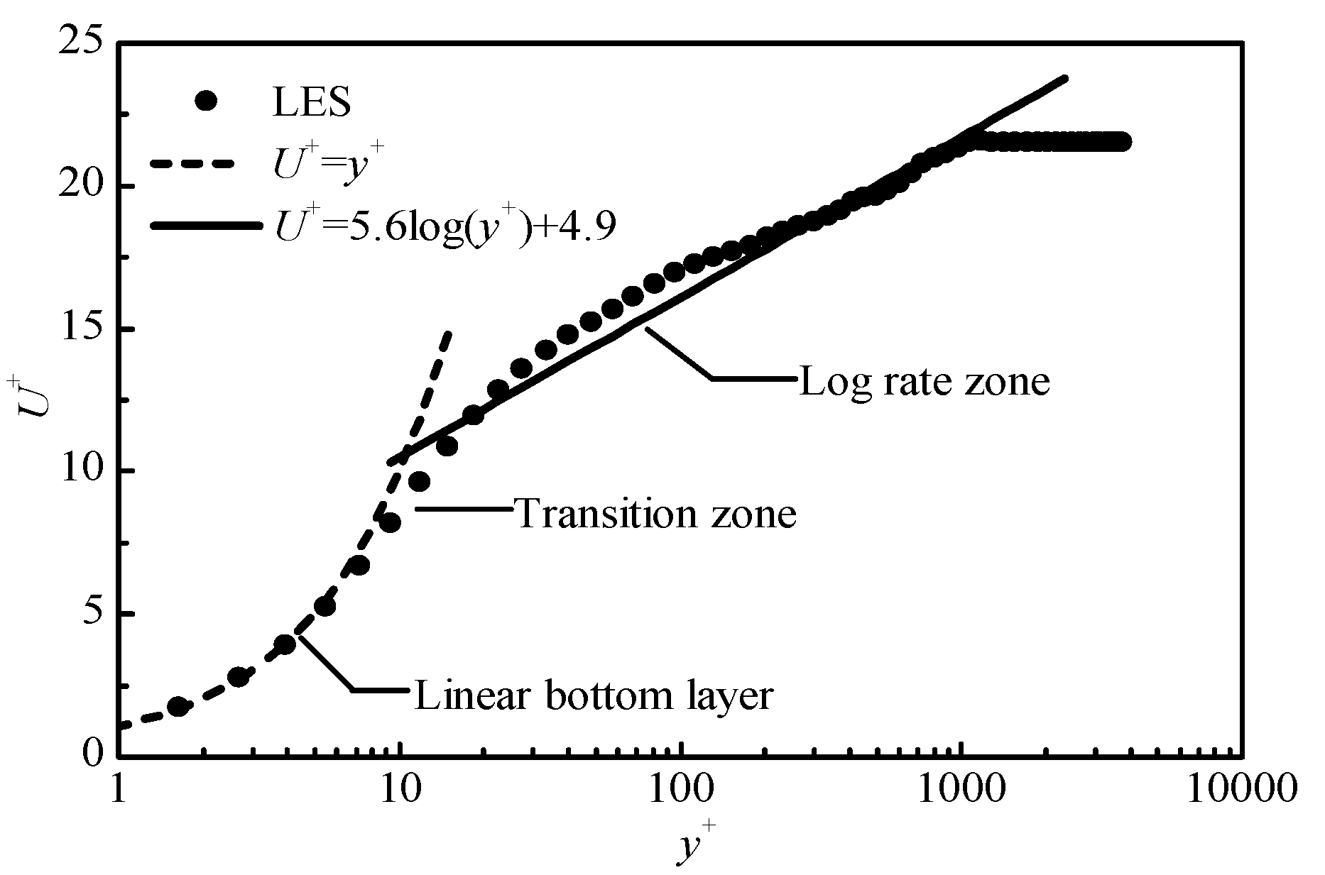
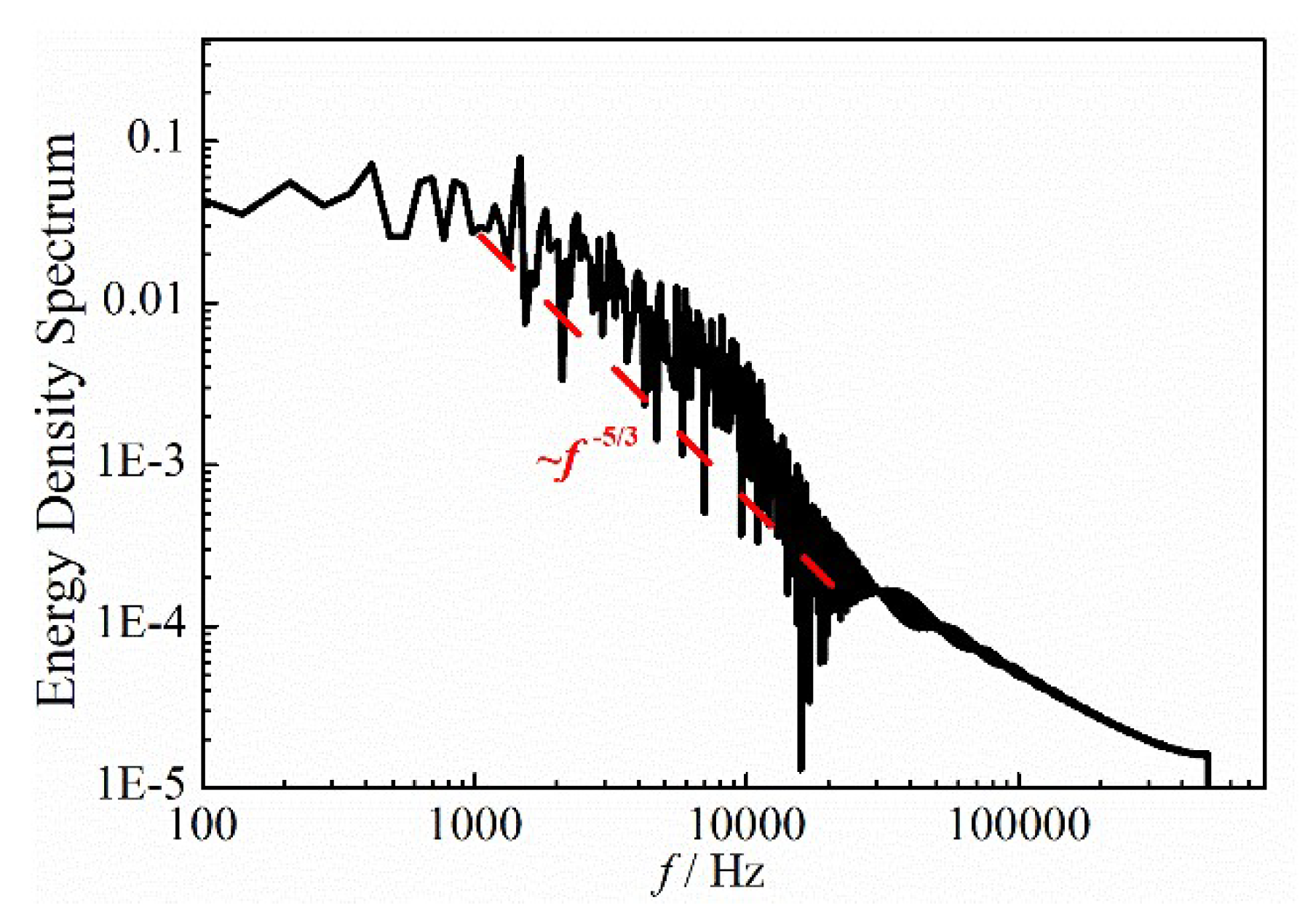
2.4. Validation of the Numerical Methods

In order to validate the numerical methodology, this study calculates a single-phase fully developed turbulent boundary layer, comparing the velocity distribution and fluctuation intensity with theoretical and DNS results, also identifying streaks and vortices which are the typical structure of a turbulent boundary layer. The simulation time was $1.6\times {10}^{-2}$ s and CPU time was $1.52\times {10}^6$ s. RMS residual was below $4\times {10}^{-6}$ for momentum and mass at every timestep. In addition, max courant number was below 0.46 at every time step. In this paper, the single-phase turbulent boundary layer is validated with the theoretical and DNS results. It also obtained the same phenomenon in vortex intensity, velocity distribution, velocity gradient, turbulent boundary thickness and turbulent kinetic energy as other studies [8].

The velocity distribution (as shown in Figure 3) is obtained by extracting and ensemble averaging the velocity data in the flow field after 20 mm downstream from the obstacle line. The aim of this process is to avoid the influence of the obstacle line. The parameters in Figure 3 are dimensionless. As the figure shows, the distribution of average velocity of the turbulent boundary layer has three typical regions: the linear bottom layer, the transitional region, and the log-rate region. The calculated results are in good agreement with the theoretical values [41,42] in both the linear bottom and logarithmic regions. The fluctuation intensity (as shown in Figure 4) is the root mean square of fluctuation velocity and can reflect the intensity of turbulence. As the figure also shows, the peak value of the fluctuation intensity occurs at a position of about $y/\delta =0.02$, and then it rapidly drops, decreasing to 0 at the edge of the boundary layer. Comparing the fluctuation intensity with the DNS results of Lund [43] and Spalart [44], it can be found that the results agree well in all three directions.

In a turbulent boundary layer, the energy is transferred from the mean flow to the fluctuation flow. Large eddies are generated by mean flow and gain energy from it. Then, the energy is transferred from large eddies to smaller eddies until the eddies are small enough in size and the energy is dissipated when the viscous forces dominate. This process is a classic energy cascade [45]. The energy spectrum shown in Figure 5 shows the energy cascade in the turbulent boundary layer. The largest eddies (lowest frequencies) on the left side of the spectrum gain energy from the mean flow and the energy cascades down to smaller eddies (larger frequencies) until it is dissipated. The streaks (as shown in Figure 6) are the streamwise distribution of high and low velocities occurring near the wall surface, which are caused by streamwise vortices and are a typical feature of the flat-plate turbulent boundary layer. Figure 6 shows the velocity profile at $y^{+}=1.5$; it is clear that the fluid begins to form streaks after it has flowed some distance from the obstacle line. The streamwise and hairpin vortices (as shown in Figure 7) are also a typical feature of the flat-plate turbulent boundary layer. In this paper, the Q-criterion is used to extract the instantaneous vortex structure, as shown in Figure 7, where $Q=4.3\times {10}^7$. The Q-criterion expression is:

$$Q=\frac{1}{2}\left({\left|\right|\mathsf{\Omega }\left|\right|}^2-{\left|\right|S\left|\right|}^2\right)$$

(23)

This represents the continuous balance of the shear strain rate and the vortex tensor, and it has a good performance in identifying vortex structures. Figure 8 shows the connection between the streaks and the streamwise vortices. It can be found that the streaks are caused by the streamwise vortices through sweep and ejection. The sweep is responsible for the increase of velocity near the wall, while ejection is responsible for the decrease. In a turbulent boundary layer, the head of the streamwise vortex would rise to the transition zone under certain conditions. At this zone it will vibrate and rupture, leading to intense fluid mixing and energy transport. In this process, a high-speed fluid will hit the wall, causing the velocity gradient near the wall to increase. These phenomena are reflected in the transition zone of the velocity distribution, in the peak of the turbulence intensity, in the gain of the energy spectrum, and the increase of frictional resistance. It is important for the method used in this study to obtain the above results, because the analysis will rely on the identification of these phenomena. From the occurrence of the burst to the increase of frictional resistance, it is a process in which various physical phenomena from micro to macro are interrelated. The most important ones among them are these we discussed above.

3. Results

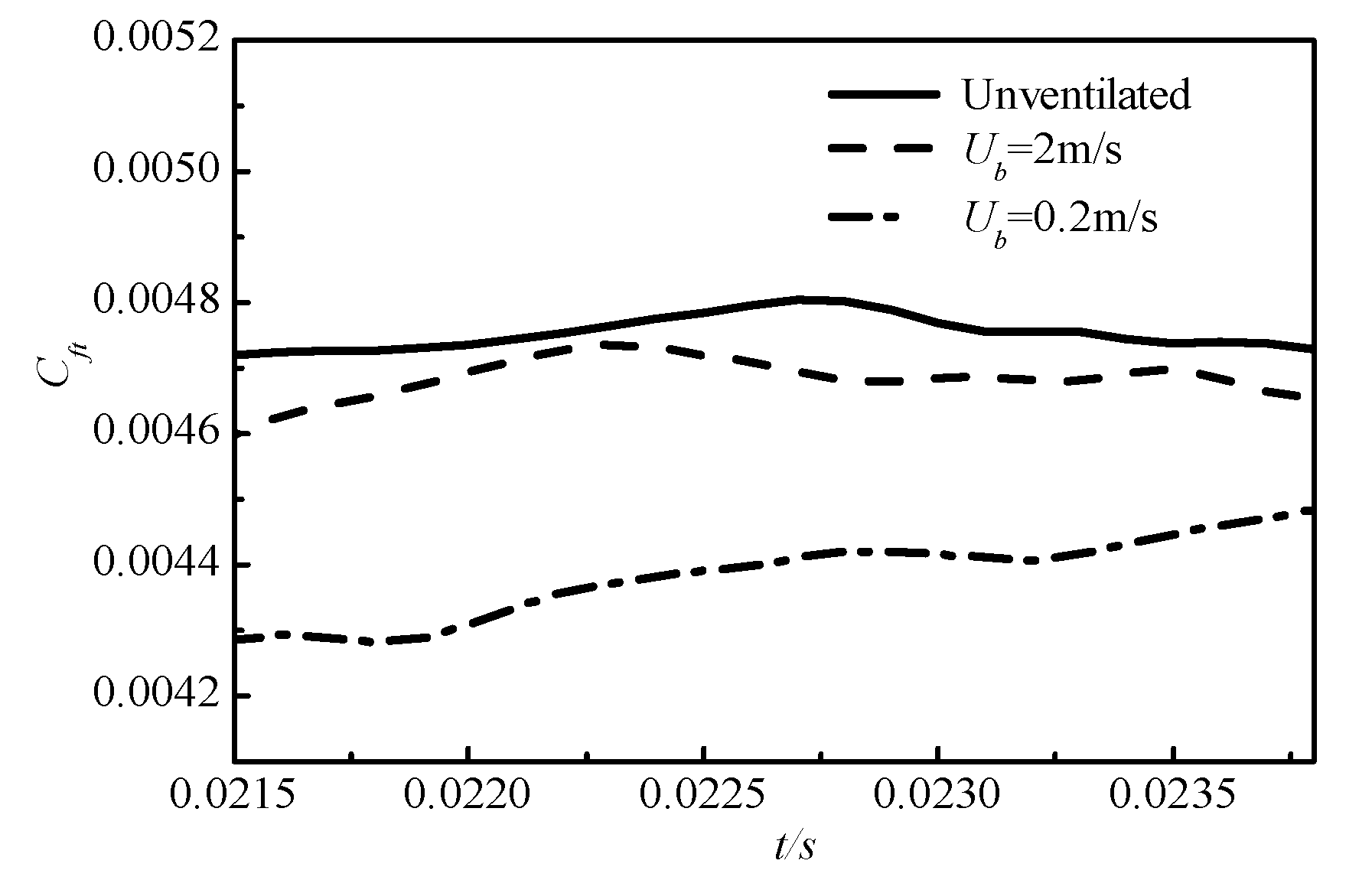
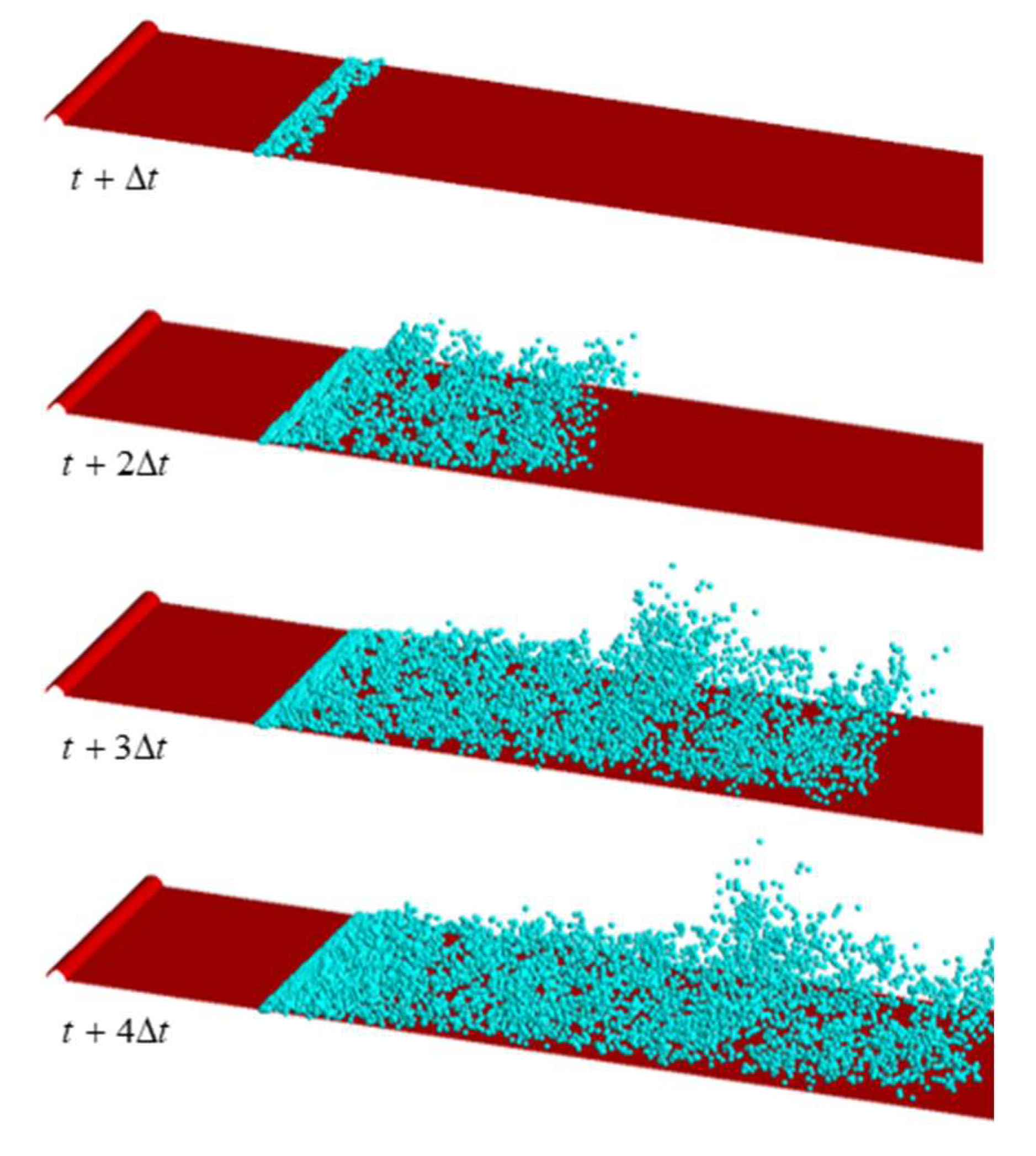
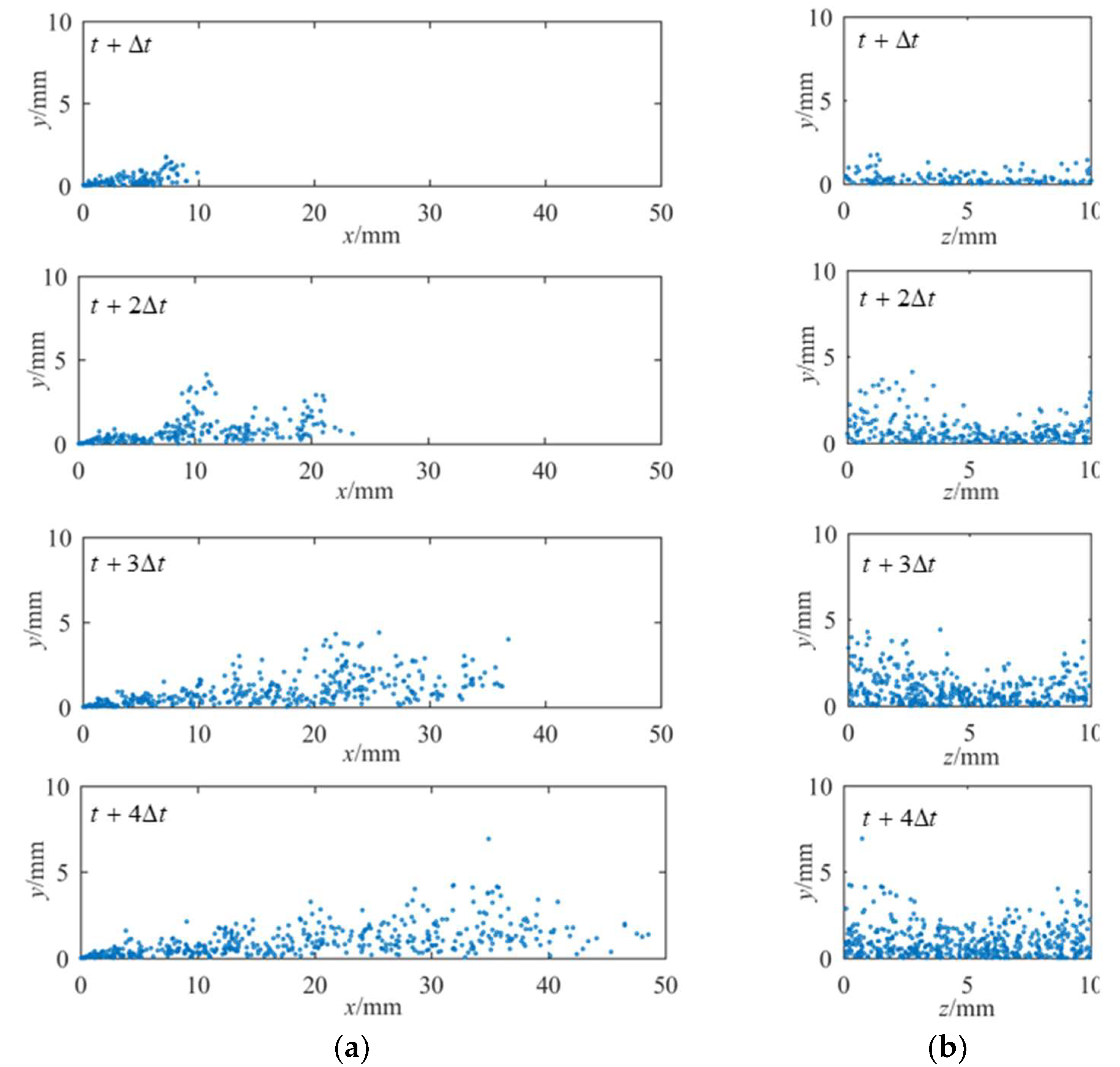
3.1. Drag Reduction and the Movement of Microbubbles

The turbulent boundary layer containing microbubbles is obtained based on the result of single-phase flat-plate turbulent boundary layer and a total of two sets of numerical simulations were performed according to Table 1. For these two cases, simulation time was $9\times {10}^{-3}$ s and CPU time was $1.84\times {10}^6$ s. RMS residual was below $4\times {10}^{-6}$ for momentum and mass at every timestep and the max courant number was below 0.46 at every time step. The drag coefficient is defined as follows [21]:

$$C_{ft}=\frac{2}{\rho U_{\infty }^2}\frac{1}{L_x{L}_z}{{\displaystyle \int }}_0^{L_x}{{\displaystyle \int }}_0^{L_z}{\tau }_w\left(x,z,t\right)dzdx$$

(24)

${\tau }_w\left(x,z,t\right)$ is the wall shear stress, and $L_x$ and $L_z$ are streamwise and spanwise lengths. Changes in the drag coefficient over time is shown in Figure 9. The drag decreases after microbubbles are introduced, and the drag reduction effect is inversely proportional to the velocity of the bubble jet. The time average of $C_{ft}$ is shown in Equation (25), and the results obtained are shown in

Table 2. Drag reduction at both injection speeds.

Case	${\mathit{U}}_{\mathit{b}}(\mathbf{m}/\mathbf{s})$	${\mathit{N}}_{\mathit{b}}\left({\mathbf{s}}^{-1}\right)$	${\mathit{C}}_{\mathit{f}}$	$\left({\mathit{C}}_{\mathit{f}0}-{\mathit{C}}_{\mathit{f}}\right)/{\mathit{C}}_{\mathit{f}0}$
A	0.2	5 × 106	4.458 × 10−3	7.34%
B	2	5 × 106	4.664 × 10−3	1.85%

.

$$C_f=\frac{1}{T}{{\displaystyle \int }}_0^T{C}_{ft}dt$$

(25)

Figure 10 shows the evolution of the microbubbles after they are injected into the turbulent boundary layer. It is clear that the microbubbles move downstream after they enter the boundary layer and have a tendency to diffuse to the outer layer. Moreover, the spatial distribution of the microbubbles is not uniform and microbubbles exhibit a random distribution. Figure 11 contains a projection onto a two-dimensional plane. It can be seen that the concentration has a gradient distribution and it first increases and then decreases in a direction perpendicular to the wall surface. The path with the highest concentration should be considered the statistical average path of the microbubbles, or their mainstream. Many microbubbles are scattered on both sides of this mainstream. It is known that many vortices are found in the turbulent boundary layer and these vortices can affect the distribution of microbubbles. These vortices are larger than the microbubbles, so they draw many microbubbles into themselves. After the microbubbles enter a vortex, they remain within it and move with it either until the vortex disappears or evolves into a smaller vortex; or, after a period of time, they escape from the vortex thanks to inertia or another factor. Microbubbles are constantly subjected to vortices, resulting in uneven distribution and scattering.

The kinetic energy of microbubbles changes over time during their movement. Figure 12a,b shows the motion trajectory and kinetic energy of 10 randomly selected microbubbles. The colors indicate the magnitudes of kinetic energy. It can be seen that changes in kinetic energy of microbubbles are irregular. After entering the flow field, some of the microbubbles rapidly increase in kinetic energy and reach a peak value, where they remain, while others continue to fluctuate.

The observation of these microbubbles shows that the kinetic energy of some microbubbles decreases as the motion of their path turns to the bottom layer after they experience the peak. At the same time, their kinetic energy increases again when they move to the outer layer. Because vortices can affect their movement, microbubbles may be entrapped, ejected to the outer layer, or drawn into the bottom layer. When they enter the outer layer, their velocities increase due to the higher fluid velocity of that layer. When they enter the bottom layer, their velocities are reduced by the deceleration of the low-velocity fluid. Thus, the kinetic energy of microbubbles fluctuates during movement.

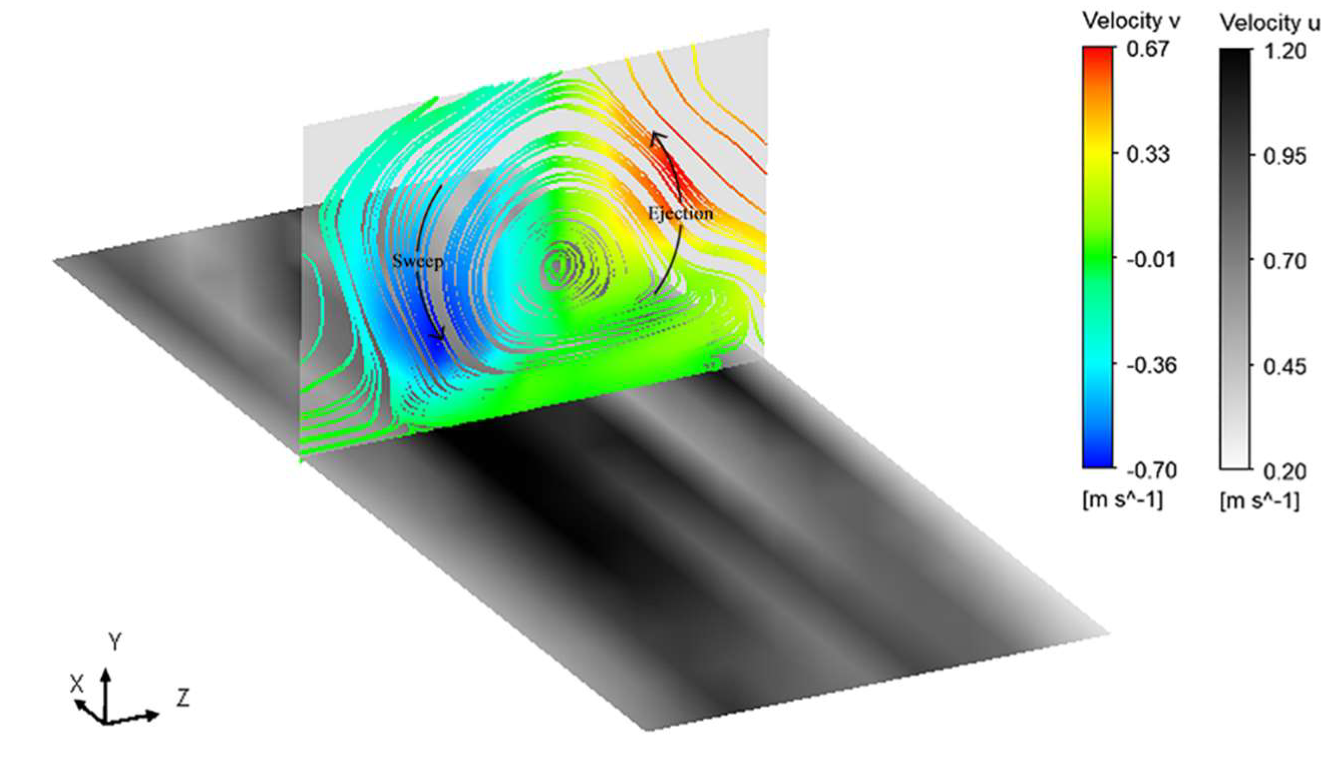
3.2. Coherent Structure Features

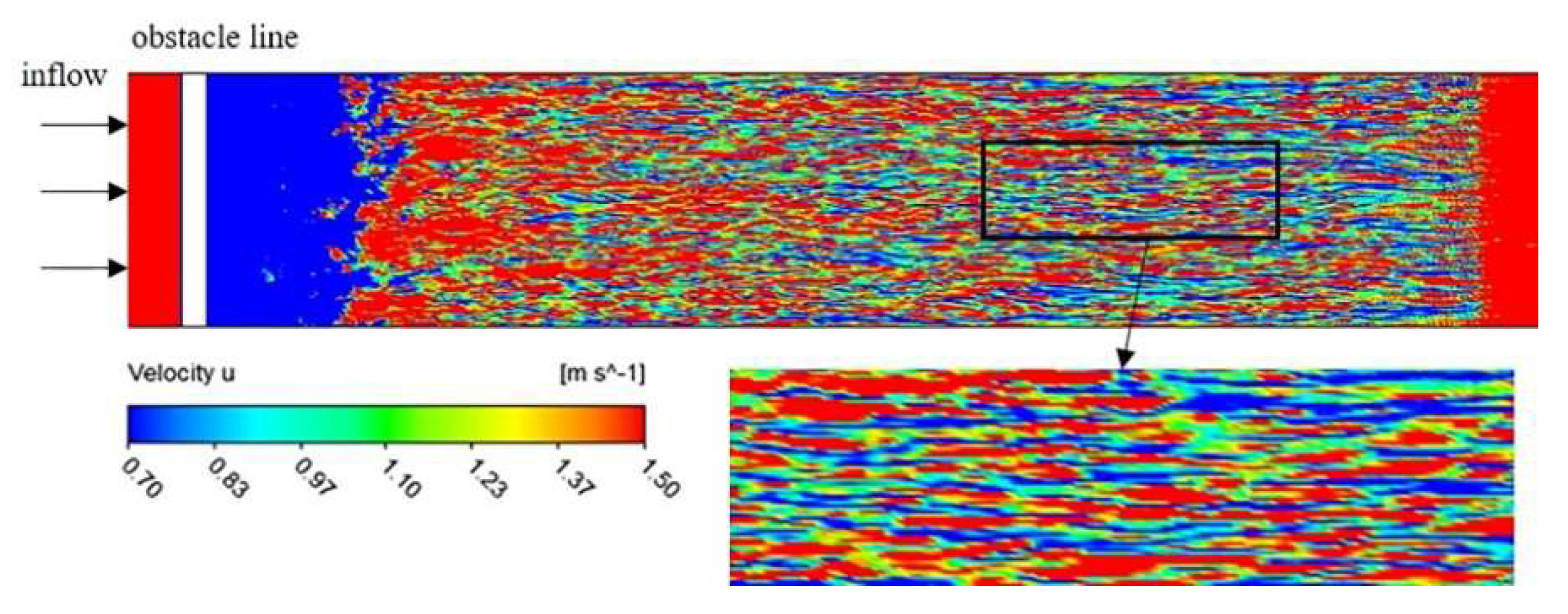
3.2.1. The Velocity Distribution

Figure 13 shows the displacement thickness from Equation (26) and momentum thickness from Equation (27) before and after the microbubbles are injected. Both show the same changes: after the microbubbles are injected, the TBL displacement thickness and momentum thickness increase. This indicates that the presence of microbubbles thickens the boundary layer. Both the TBL displacement thickness and momentum thickness are related to velocity distribution. When the velocity gradient in the boundary layer is large, and the change is severe, the velocity quickly reaches that of the inflow, reducing the TBL thickness, and when it is small, the reverse happens.

The effects of microbubbles on the TBL velocity distribution are shown in Figure 14. Panel (a) shows the distribution of the velocity gradient within the boundary layer. It can be seen that the velocity gradient at the wall is reduced after the injection of bubbles, which can explain the reduction in drag coefficient because the skin friction is determined by the velocity gradient at the wall. Furthermore, because the velocity of the wall is always zero, the velocity gradient is only related to the flow velocity near the wall. If the incoming velocity remains constant, the velocity near the wall is determined by the vortex structure and burst [36,37]. On the sweep side of the vortex, the fluid impacts the wall at high speed, increasing velocity at that point. Meanwhile, when the vortex breaks, that is, when a burst occurs, the fluid also impacts the wall at high speed, increasing the velocity near the wall. Taking these considerations into account, it can be assumed that the presence of the microbubbles affects the vortex structure and burst. In fact, Ferrante and Elghobashi [8] conducted a series of studies on vortex structures, and found that after the injection of microbubbles, a positive velocity gradient is generated, due to the presence of a concentration gradient. This results in a velocity component that is perpendicular to the wall surface, which pushes the vortex structure away from the wall. Thus, the strength of the impact of the high-speed fluid on the surface of the wall is weakened, and the velocity near the wall is lower than before, so the velocity gradient at the wall is reduced. Further, because the rupture of the vortex is the cause of a rapid change in the velocity distribution, the outward movement of the vortex structure causes the region of velocity change to move promptly outward, as shown in Figure 14b.

$${\delta }^{*}={{\displaystyle \int }}_0^{\infty }\left(1-\frac{u}{u_{\infty }}\right)dy$$

(26)

$$\theta ={{\displaystyle \int }}_0^{\infty }\frac{u}{u_{\infty }}\left(1-\frac{u}{u_{\infty }}\right)dy$$

(27)

3.2.2. The Vortex Structure Intensity

Burst denotes the phenomenon of the instability and rupture of a vortex, for which it is necessary to study the distribution of vortex intensity and the changes caused by microbubbles. The most commonly used methods for identifying vortices are those incorporating the ${\lambda }_2$-value or Q-criteria. The ${\lambda }_2$ is the second-largest eigenvalue of the tensor $S_{ik}{S}_{ki}+{\mathsf{\Omega }}_{ik}{\mathsf{\Omega }}_{kj}$, where $S_{ij}=\left({\partial }_j{U}_i+{\partial }_i{U}_j\right)/2$ is the strain-rate tensor, and ${\mathsf{\Omega }}_{ij}=\left({\partial }_j{U}_i-{\partial }_i{U}_j\right)/2$ is the rotation-rate tensor. $Q=\left({\left|\right|\mathsf{\Omega }\left|\right|}^2-{\left|\right|S\left|\right|}^2\right)/2$ represents the continuous equilibrium of the shear strain rate and vortex tensor, and this expression has a good record of identifying vortices.

The distribution of the root mean square of ${\lambda }_2$ and Q values along the normal direction are shown in Figure 15. Both methods identify the same vortex intensity distribution. Comparing the changes before and after injecting microbubbles, the injection of microbubbles leads to the weakening of the vortex intensity. Figure 15 shows that the intensity of the vortex weakens in the vicinity of the peak. The peak position is approximately $18<y^{+}<40$, which corresponds to the transition zone in Figure 3. The distribution of turbulent fluctuation intensity that appears in Figure 4 has a peak exactly where the peak of fluctuation intensity is located. From the literature [46,47], it can be deduced that this is the position where the burst occurs. In other words, the peak position in Figure 15 is where the burst occurs. Thus, the decrease in the peak value of the vortex intensity after the injection of microbubbles indicates that the appearance of microbubbles may suppress the occurrence of the burst.

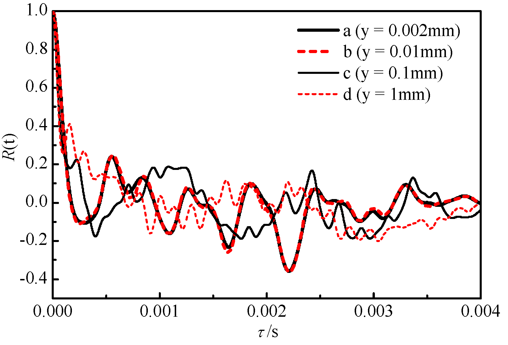
3.2.3. The Burst Frequency

The analysis of velocity gradient and vortex intensity shows that the presence of microbubbles may suppress the occurrence of a burst. To further address this speculation, it is necessary to discuss a burst in detail. A burst is a quasi-periodic process involving rising of a vortex, vibration, rupture, and sweeping. It is uncertain what triggers it, but once it is triggered, it evolves in the fixed order, from the rising of vortex to sweeping and is thus called a coherent structure [48,49,50,51]. After a burst, there is a period of calm, or a new burst is triggered immediately. Because bursts occur on a microscopic scale, and hundreds of bursts occur simultaneously in a turbulent boundary layer, it is difficult to observe them directly. In general, bursts can be detected by the characteristic signals they emit. This study detects the frequency of bursts using the autocorrelation function of velocity. This method comes from the literature [46,52,53], which suggests that the autocorrelation function of velocity can be used to detect the interval of bursts and it can effectively compensate for the deficiency of the conditional sampling method because there is no need to artificially provide a basis for discrimination.

The correlation of the time series signal $x\left(t\right)$ at different time intervals is called the autocorrelation function of the time series signal, and its expression is as follows:

$$R\left(t,\tau \right)=E\left[x\left(t\right)x\left(t+\tau \right)\right]$$

(28)

where E indicates an ensemble average of samples. Figure 16 is an autocorrelation of flow velocity at monitoring points in the flow field. The distances between the position of the monitoring points and the wall increases from points a to d. In the figure, the horizontal axis indicates the delay time, and the delay time corresponding to the second peak of $R\left(t\right)$ is the period of the bursts [46,52,53]. As shown in the figure, the autocorrelation of velocity at points a and b remains the same. A second peak was reached at 0.56 ms, indicating that bursts occur at a period of 0.56 ms. The delay time for $R\left(t\right)$ at point c to reach the second peak is 0.94 ms. This period of the bursts is longer than that at point b, which means that at some distance from the wall, bursts occur less frequently than near it. Point d is chosen completely randomly, and there is no quasi-periodic phenomenon, which indicates that no bursts occur. It should be noted that a quasi-periodic phenomenon is also detected at point a, and the changes in points a and b are almost identical, but bursts do not occur at point a. One reason why the change at a is identical to that at point b is that so long as bursts occur at point b, a high-speed fluid can impact the wall, and point a is exactly where the high-speed fluid passes. Another reason is that point a is close to the wall and bursts mainly occur in the transition zone. Therefore, a quasi-periodic change can be detected at point a, although no bursts occur there.

$$(U_b=2\mathrm{m}/\mathrm{s},x=30\mathrm{mm},z=5\mathrm{mm}).$$

The above analysis shows that due to the complexity of the situation, many factors affect the detection of bursts. Periods of bursts at different locations are very different, and the trigger for any given burst is uncertain. To eliminate the error caused by this uncertainty as much as possible, this paper monitors velocity time series of 20 locations. For each position, the periods of bursts are identified using the autocorrelation method and then averaged to obtain an average burst period. By calculation, the average burst frequency before the injection of microbubbles is 637.8 Hz, and the average frequency after injection is 611.2 Hz, which indicates that the presence of microbubbles reduces the frequency of bursts.

3.3. Transport of Turbulent Kinetic Energy

Because bursts can cause strong fluid fluctuation and energy transport, to further explore the changes caused by microbubbles, this study next examines the transport of turbulent kinetic energy. Taking the result of $U_b=2\mathrm{m}/\mathrm{s}$ as an example, a turbulent boundary layer containing microbubbles was analyzed. In this layer, turbulence obtains energy from the mean flow. The energy is then gradually transferred from large-scale to smaller-scale vortices until the vortices are no longer small, and the energy from the smallest-scale vortex is converted into heat and dissipated.

$$k=\frac{1}{2}\overline{u_i^{\prime 2}}$$

(29)

$$p=-\overline{u_i^{\prime }{u}_j^{\prime }}\frac{\partial \overline{u_i}}{\partial x_j}$$

(30)

$$\epsilon =\nu \overline{\left(\frac{\partial u_i^{\prime }}{\partial x_j}+\frac{\partial u_j^{\prime }}{\partial x_i}\right)}\frac{\partial u_j^{\prime }}{\partial x_i}$$

(31)

Figure 17a gives a comparison of turbulent kinetic energy as expressed in Equation (29), before and after the injection of microbubbles, which shows the kinetic energy of the fluid fluctuation per unit mass. The figure shows that turbulent energy is reduced after the injection of microbubbles. This is because the source of turbulent energy is the mean flow, and bursts are an important mechanism for the transfer of energy from mean to fluctuating flow. After the streak is destabilized, it oscillates violently, and the fluid in the linear bottom layer is ejected to the logarithmic layer, while the logarithmic layer of fluid is brought to the bottom layer in a high-speed sweep. During this process, a strong fluctuation occurs, and energy is transferred from the mean to the fluctuating flow. The presence of microbubbles suppresses the frequency of bursts in the turbulent boundary layer, which is equivalent to closing the channel through which energy is transferred from the mean to the fluctuating flow. The energy obtained from the fluctuating flow is reduced, resulting in a decrease in kinetic energy. This decrease in energy is reflected in vortex intensity, which results in a decrease in the intensity of the vortex in Figure 15. Figure 17b shows components of turbulent kinetic energy. The reduction in turbulent kinetic energy is mainly provided by streamwise and spanwise components, while the normal components are almost the same. This shows that the presence of microbubbles does not affect normal turbulent kinetic energy.

The production term P of the turbulent kinetic energy from Equation (30) reflects the acquisition of turbulent kinetic energy. The equation contains the Reynolds stress term and the average strain rate, which represents the deformation work performed by the Reynolds stress on the average deformation rate. $P>0$ means that energy is transferred from the mean to the fluctuating flow. $P<0$ means that energy is transferred from the fluctuating to the mean flow. Figure 18a compares the distribution of the production term of the turbulent energy in the normal direction before and after the injection of the microbubbles. It can be seen that the peak value of the production is reduced after the microbubbles are injected, which means that the reduction of turbulent kinetic energy comes from the decrease of production.

The dissipative term $\epsilon$ of the turbulent kinetic energy in Equation (31) reflects the loss of kinetic energy. It is the product of the rate of fluctuating viscous stress and the fluctuating strain, representing energy dissipation due to viscous action. Figure 18b compares the distribution of the energy dissipation term along the normal direction before and after the introduction of microbubbles. The values are roughly the same, which means that the presence of microbubbles does not affect the dissipation of turbulent energy.

4. Discussion

This study examined the microscopic mechanisms of MDR in a fully developed turbulent boundary layer over a flat-plate. In this section, the results of this study are discussed and the connection with other research is raised. Because prior research has found that sweeping, the last event in the burst process, increases the streamwise velocity near the wall, it can be speculated that the presence of microbubbles may suppress bursts to obtain the low skin friction. This speculation is confirmed by the reduction of bursts frequency from 637.8 Hz to 611.2 Hz and the reduction of velocity gradient at the wall surface. At the same time, the reduction of bursts frequency also decreases the intensity of vortex because bursts lead to drastic fluid fluctuation. It subsequently reduces the production of turbulent kinetic energy.

The studies by Ferrante and Elghobashi [8,21] revealed that the presence of microbubbles drives the vortex structure to move away from the wall. In this way, the impact force of sweep on the wall surface is much smaller when the fluid reaches the wall, thereby reducing the frictional drag. Combined with the results of this study, it can be found that the presence of microbubbles both drives the vortex structure away from the wall and suppresses the bursts frequency. Hence, the sweeping reduces both in frequency and strength.

This paper focused on bursts to investigate the microscopic mechanisms of MDR and found that the reduction of burst frequency lessens the skin friction. As for future work, more analysis considering the flow structures, such as vortices and the streak, and their interaction with microbubbles would be beneficial for a comprehensive understanding of MDR. Additional work is underway to investigate how this interaction works.

5. Conclusions

In this paper, a numerical simulation of microbubbles is carried into the flat-plate turbulent boundary layer, and the relationship between microbubbles and turbulent coherent structures is analyzed. Furthermore, the internal mechanism of microbubble drag reduction is discussed. The main conclusions and findings of this study are as follows.

(1)

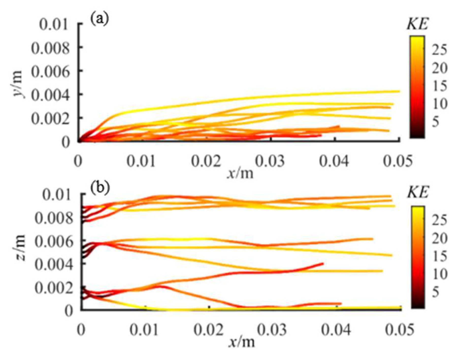
The path of microbubbles shuttles back and forth between the bottom and outer layers of the turbulent boundary layer. Meanwhile, the kinetic energy of the microbubbles rises at the outer layer and decreases at the bottom layer due to the difference in flow velocity between the bottom and outer layers.

(2)

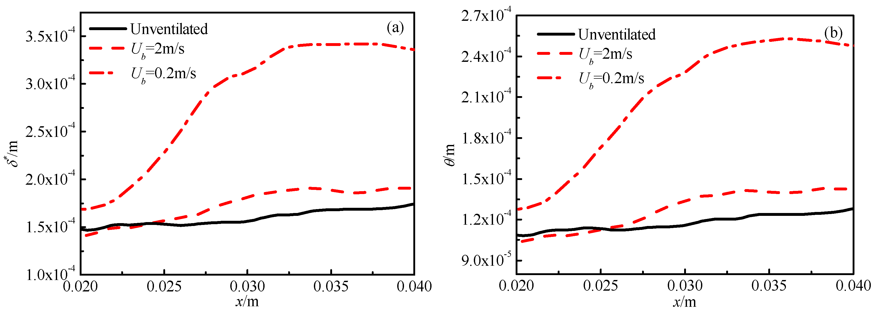
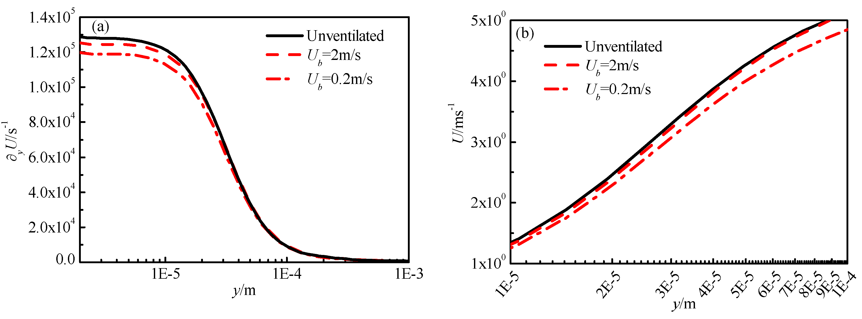
The velocity gradient at the wall is decreased after the injection of microbubbles. At the same time, the region where the mean velocity promptly changes moves outward after injection. Because of these two changes, a longer distance is required for the velocity in the turbulent boundary layer to reach the inflow velocity. Thus, the displacement thickness and momentum thickness increase and the turbulent boundary layer becomes thicker.

(3)

The average burst frequency decreases from 637.8 Hz to 611.2 Hz after the injection of microbubbles, which leads to a decrease in the velocity gradient at the wall. Because sweeping, the last event in the burst process, contributes to the high velocity near the wall, the decrease in burst frequency means that the velocity near the wall is lowered, which leads to a decrease in the velocity gradient.

(4)

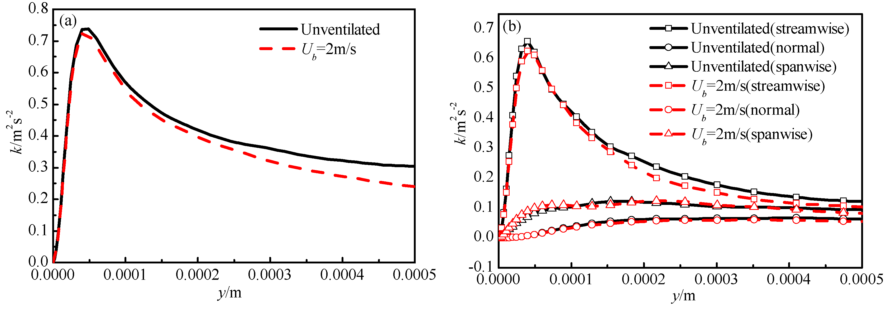
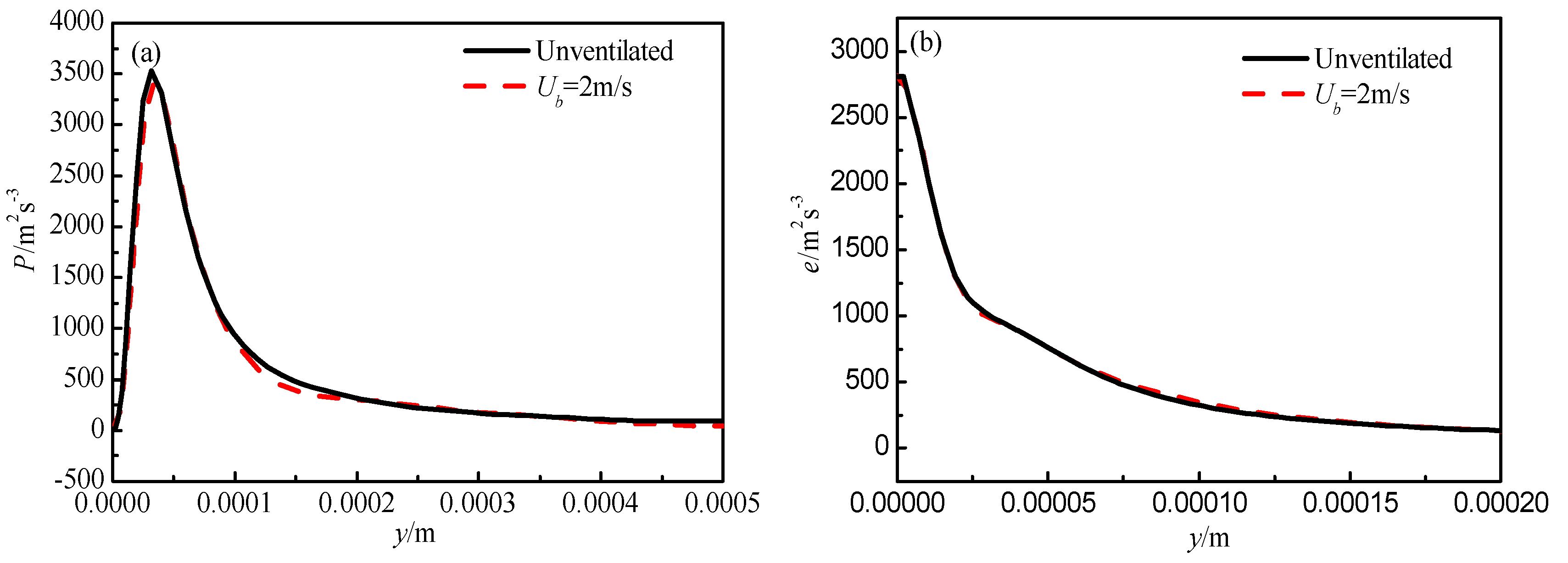
The reduction of burst frequency also, with the fluid fluctuation reduced in degree, decreases the intensity of vortices near the wall, leading to reduced production of turbulent kinetic energy. Furthermore, the reduced production makes the streamwise and spanwise components of turbulent kinetic energy decrease, and the normal component remains unchanged.

References

1. Guin, M.M.; Kato, H.; Yamaguchi, H.; Maeda, M.; Miyanaga, M. Reduction of skin friction by microbubbles and its relation with near-wall bubble concentration in a channel. J. Mar. Sci. Technol. 1996, 1, 241–254. [Google Scholar] [CrossRef]
2. Choi, H.; Moin, P.; Kim, J. Active turbulence control for drag reduction in wall-bounded flows. J. Fluid Mech. 1994, 262, 75–110. [Google Scholar] [CrossRef]
3. Xu, J.; Maxey, M.R.; Karniadakis, G.E. Numerical simulation of turbulent drag reduction using micro-bubbles. J. Fluid Mech. 2002, 468, 271–281. [Google Scholar] [CrossRef] [Green Version]
4. Sanders, W.C.; Winkel, E.S.; Dowling, D.R.; Perlin, M.; Ceccio, S.L. Bubble friction drag reduction in a high-Reynolds-number flat-plate turbulent boundary layer. J. Fluid Mech. 2006, 552, 353–380. [Google Scholar] [CrossRef]
5. Chung, Y.M.; Talha, T. Effectiveness of active flow control for turbulent skin friction drag reduction. Phys. Fluids 2011, 23, 025102. [Google Scholar] [CrossRef]
6. Deng, B.-Q.; Xu, C.-X. Influence of active control on STG-based generation of streamwise vortices in near-wall turbulence. J. Fluid Mech. 2012, 710, 234–259. [Google Scholar] [CrossRef]
7. Jiang, C.-X.; Li, S.-L.; Li, F.-C.; Li, W.-Y. Numerical study on axisymmetric ventilated supercavitation influenced by drag-reduction additives. Int. J. Heat Mass Transf. 2017, 115, 62–76. [Google Scholar] [CrossRef]
8. Ferrante, A.; Elghobashi, S. On the physical mechanisms of drag reduction in a spatially developing turbulent boundary layer laden with microbubbles. J. Fluid Mech. 2004, 503, 345–355. [Google Scholar] [CrossRef]
9. Mccormick, M.E.; Bhattacharyya, R. Drag reduction of a submersible hull by electrolysis. Nav. Eng. J. 1973, 85, 11–16. [Google Scholar] [CrossRef]
10. Madavan, N.; Deutsch, S.; Merkle, C. Reduction of turbulent skin friction by microbubbles. Phys. Fluids 1984, 27, 356–363. [Google Scholar] [CrossRef]
11. Merkle, C.; Deutsch, S. Microbubble drag reduction. In Frontiers in Experimental Fluid Mechanics; Springer: Berlin/Heidelberg, Germany, 1989; pp. 291–335. [Google Scholar]
12. Kawamura, T.; Moriguchi, Y.; Kato, H.; Kakugawa, A.; Kodama, Y. Effect of bubble size on the microbubble drag reduction of a turbulent boundary layer. In Proceedings of the ASME/JSME 2003 4th Joint Fluids Summer Engineering Conference, Honolulu, HI, USA, 6–10 July 2003; pp. 647–654. [Google Scholar]
13. Shen, X.; Ceccio, S.L.; Perlin, M. Influence of bubble size on micro-bubble drag reduction. Exp. Fluids 2006, 41, 415–424. [Google Scholar] [CrossRef]
14. Fontaine, A.A.; Deutsch, S. The influence of the type of gas on the reduction of skin friction drag by microbubble injection. Exp. Fluids 1992, 13, 128–136. [Google Scholar] [CrossRef]
15. Zhao, X.-j.; Zong, Z.; Jiang, Y.-c.; Pan, Y. Numerical simulation of micro-bubble drag reduction of an axisymmetric body using OpenFOAM. J. Hydrodyn. 2019, 31, 900–910. [Google Scholar] [CrossRef]
16. Song, W.; Wang, C.; Wei, Y.; Zhang, X.; Wang, W. Experimental study of microbubble drag reduction on an axisymmetric body. Mod. Phys. Lett. B 2018, 32, 1850035. [Google Scholar] [CrossRef]
17. Bogdevich, V.; Evseev, A.; Malyuga, A.; Migirenko, G. Gas-saturation effect on near-wall turbulence characteristics. In Proceedings of the 2nd International BHRA Fluid Drag Reduction Conference, Cambridge, UK, 31 August 1977. [Google Scholar]
18. Legner, H.H. A simple model for gas bubble drag reduction. Phys. Fluids 1984, 27, 2788–2790. [Google Scholar] [CrossRef]
19. Madavan, N.; Merkle, C.; Deutsch, S. Numerical investigations into the mechanisms of microbubble drag reduction. J. Fluids Eng. 1985, 107, 370–377. [Google Scholar] [CrossRef]
20. Kanai, A.; Miyata, H. Direct numerical simulation of wall turbulent flows with microbubbles. Int. J. Numer. Methods Fluids 2001, 35, 593–615. [Google Scholar] [CrossRef]
21. Ferrante, A.; Elghobashi, S. Reynolds number effect on drag reduction in a microbubble-laden spatially developing turbulent boundary layer. J. Fluid Mech. 2005, 543, 93–106. [Google Scholar] [CrossRef]
22. Zhang, X.; Wang, J.; Wan, D. Euler–Lagrange study of bubble drag reduction in turbulent channel flow and boundary layer flow. Phys. Fluids 2020, 32, 027101. [Google Scholar]
23. Elbing, B.R.; Mäkiharju, S.; Wiggins, A.; Perlin, M.; Dowling, D.R.; Ceccio, S.L. On the scaling of air layer drag reduction. J. Fluid Mech. 2013, 717, 484–513. [Google Scholar] [CrossRef]
24. Elbing, B.R.; Winkel, E.S.; Lay, K.A.; Ceccio, S.L.; Dowling, D.R.; Perlin, M. Bubble-induced skin-friction drag reduction and the abrupt transition to air-layer drag reduction. J. Fluid Mech. 2008, 612, 201–236. [Google Scholar] [CrossRef]
25. Yu, X.; Wang, Y.; Huang, C.; Wei, Y.; Fang, X.; Du, T.; Wu, X. Experiment and simulation on air layer drag reduction of high-speed underwater axisymmetric projectile. Eur. J. Mech.-B/Fluids 2015, 52, 45–54. [Google Scholar] [CrossRef] [Green Version]
26. Ceccio, S.L. Friction drag reduction of external flows with bubble and gas injection. Annu. Rev. Fluid Mech. 2010, 42, 183–203. [Google Scholar] [CrossRef]
27. Du, T.; Wang, Y.; Liao, L.; Huang, C. A numerical model for the evolution of internal structure of cavitation cloud. Phys. Fluids 2016, 28, 077103. [Google Scholar] [CrossRef]
28. Long, X.; Cheng, H.; Ji, B.; Arndt, R.E.; Peng, X. Large eddy simulation and Euler–Lagrangian coupling investigation of the transient cavitating turbulent flow around a twisted hydrofoil. Int. J. Multiph. Flow 2018, 100, 41–56. [Google Scholar] [CrossRef]
29. Nicoud, F.; Ducros, F. Subgrid-scale stress modelling based on the square of the velocity gradient tensor. Flow Turbul. Combust. 1999, 62, 183–200. [Google Scholar] [CrossRef]
30. Germano, M.; Piomelli, U.; Moin, P.; Cabot, W.H. A dynamic subgrid-scale eddy viscosity model. Phys. Fluids A Fluid Dyn. 1991, 3, 1760–1765. [Google Scholar] [CrossRef]
31. Lilly, D.K. A proposed modification of the Germano subgrid-scale closure method. Phys. Fluids A Fluid Dyn. 1992, 4, 633–635. [Google Scholar] [CrossRef]
32. Apte, S.; Mahesh, K.; Lundgren, T. A Eulerlan-Lagrangian Model to Simulate Two-Phase/Particulate Flows; Minnesota Univ Minneapolis: Minneapolis, MN, USA, 2003. [Google Scholar]
33. Patel, R.G.; Desjardins, O.; Kong, B.; Capecelatro, J.; Fox, R.O. Verification of Eulerian–Eulerian and Eulerian–Lagrangian simulations for turbulent fluid–particle flows. AIChE J. 2017, 63, 5396–5412. [Google Scholar] [CrossRef]
34. Hoppe, F.; Breuer, M. A deterministic and viable coalescence model for Euler–Lagrange simulations of turbulent microbubble-laden flows. Int. J. Multiph. Flow 2018, 99, 213–230. [Google Scholar] [CrossRef]
35. Asiagbe, K.S.; Fairweather, M.; Njobuenwu, D.O.; Colombo, M. Large eddy simulation of microbubble transport in a turbulent horizontal channel flow. Int. J. Multiph. Flow 2017, 94, 80–93. [Google Scholar] [CrossRef] [Green Version]
36. Zhang, Z.; Cui, G.; Xu, C. Theory and Modeling of Turbulence; Tsinghua University Press: Beijing, China, 2005; Volume 80, p. 81. [Google Scholar]
37. Zhang, Z.; Cui, G.; Xu, C. The Theory and Application of Large-Eddy Simulation of Turbulence; Tsinghua University Press: Beijing, China, 2008. [Google Scholar]
38. Clauser, F.H. The turbulent boundary layer. Adv. Appl. Mech. 1956, 4, 1–51. [Google Scholar]
39. Orlandi, P.; Pirozzoli, S.; Bernardini, M. DNS of laminar-turbulent boundary layer transition induced by solid obstacles. arXiv 2015, arXiv:1503.08614. [Google Scholar]
40. Zhang, L.-x.; Chen, M.; Deng, J.; Shao, X.-m. Experimental and numerical studies on the cavitation over flat hydrofoils with and without obstacle. J. Hydrody. 2019, 31, 708–716. [Google Scholar] [CrossRef]
41. Coles, D. The law of the wake in the turbulent boundary layer. J. Fluid Mech. 1956, 1, 191–226. [Google Scholar] [CrossRef] [Green Version]
42. Schlichting, H.; Gersten, K. Boundary-Layer Theory; Springer: Berlin/Heidelberg, Germany, 2016. [Google Scholar]
43. Lund, T.S.; Wu, X.; Squires, K.D. Generation of turbulent inflow data for spatially-developing boundary layer simulations. J. Comput. Phys. 1998, 140, 233–258. [Google Scholar] [CrossRef] [Green Version]
44. Spalart, P.R. Direct simulation of a turbulent boundary layer up to R θ = 1410. J. Fluid Mech. 1988, 187, 61–98. [Google Scholar] [CrossRef]
45. Pope, S.B. Turbulent Flows; IOP Publishing: Bristol, UK, 2001. [Google Scholar]
46. Kim, H.; Kline, S.; Reynolds, W. The production of turbulence near a smooth wall in a turbulent boundary layer. J. Fluid Mech. 1971, 50, 133–160. [Google Scholar] [CrossRef]
47. Klebanoff, P. Characteristics of turbulence in a boundary layer with zero pressure gradient. NACA Tech. Note 1954, 1247, 8–35. [Google Scholar]
48. Shekar, A.; Graham, M.D. Exact coherent states with hairpin-like vortex structure in channel flow. J. Fluid Mech. 2018, 849, 76–89. [Google Scholar] [CrossRef] [Green Version]
49. Maciel, Y.; Simens, M.P.; Gungor, A.G. Coherent structures in a non-equilibrium large-velocity-defect turbulent boundary layer. Flow Turbul. Combust. 2017, 98, 1–20. [Google Scholar] [CrossRef]
50. Silvestri, A.; Ghanadi, F.; Arjomandi, M.; Cazzolato, B.; Zander, A.; Chin, R. Mechanism of sweep event attenuation using micro-cavities in a turbulent boundary layer. Phys. Fluids 2018, 30, 055108. [Google Scholar] [CrossRef]
51. Robinson, S.K. Coherent motions in the turbulent boundary layer. Annu. Rev. Fluid Mech. 1991, 23, 601–639. [Google Scholar] [CrossRef]
52. Strickland, J.; Simpson, R.L. ’’Bursting’’frequencies obtained from wall shear stress fluctuations in a turbulent boundary layer. Phys. Fluids 1975, 18, 306–308. [Google Scholar] [CrossRef]
53. Nan, J.; Zhendong, W. Detection of average burst period in wall turbulence by means of autocorrelation. J. Exp. Mech. 1995, 10, 343–348. [Google Scholar]
Figure 1. Schematic of geometrical and boundary conditions.
Jmse 08 00524 g001
Figure 2. Magnified view of mesh near the obstacle line. Δ y + = 0.7 , Δ x + = 37 and Δ z + = 18 at the plate. The mesh is evenly distributed in the streamwise and spanwise directions and becomes dense in the near-wall area in the normal direction. The amount of global mesh is 6.88 million.
Jmse 08 00524 g002
Figure 3. Comparison of Large Eddy Simulation (LES) and theoretical values [41,42] for turbulent boundary layer velocity distribution. The data are extracted from the area below 20 mm downstream from the obstacle line and are shown after ensemble averaging.
Jmse 08 00524 g003
Figure 4. Comparison of LES and Direct Numerical Simulation (DNS) [43,44] for fluctuation intensity distribution (a) streamwise, (b) normal, and (c) spanwise. The data shown are extracted from the area below 20 mm downstream from the obstacle line.
Jmse 08 00524 g004
Figure 5. Plot of Energy Density Spectrum. The largest eddies (lowest frequencies) on the left side of the spectrum gained energy from the mean flow and the energy cascades down to smaller eddies (larger frequencies) until it is dissipated.
Jmse 08 00524 g005
Figure 6. Streaks at y + = 1.5 . Streaks are a typical feature of the flat-plate turbulent boundary layer. They are caused by a streamwise vortex.
Jmse 08 00524 g006
Figure 7. Instantaneous iso-surface of Q = 4.3 × 10 7 . The streamwise and hairpin vortices are typical features of the flat-plate turbulent boundary layer.
Jmse 08 00524 g007
Figure 8. Connection between the streaks and the streamwise vortex. The sweep event increases the velocity near the wall, causing the high-speed streak, while the ejection decreases the velocity, causing the low-speed streak.
Jmse 08 00524 g008
Figure 9. Drag coefficient of the flat plate at both injection speeds. The data shown were extracted from the plate below 20 mm downstream from the obstacle line.
Jmse 08 00524 g009
Figure 10. Distribution of microbubbles at four different moments. The quantity rate of microbubbles is 5 × 10⁶ s−1. Their size is set to a normal distribution with a standard deviation of 1.
Jmse 08 00524 g010
Figure 11. Projection of microbubble distribution on an x–y plane (a) and a z–y plane (b) at four different moments.
Jmse 08 00524 g011
Figure 12. Trajectory and changes in kinetic energy of 10 randomly selected microbubbles: (a) projection on an x–y plane and (b) projection on an x–z plane.
Jmse 08 00524 g012
Figure 13. Streamwise variation in displacement thickness and momentum thickness of the boundary layer: (a) displacement thickness and (b) momentum thickness.
Jmse 08 00524 g013
Figure 14. Profiles of mean velocity gradient and mean velocity: (a) mean velocity gradient and (b) mean velocity.
Jmse 08 00524 g014
Figure 15. (a) Average distribution of the root mean square of λ 2 along the normal direction and (b) average distribution of root mean square of Q along the normal direction.
Jmse 08 00524 g015
Figure 16. Streamwise velocity autocorrelation at monitoring points.
Jmse 08 00524 g016
Figure 17. Average distribution of turbulent kinetic energy along the normal direction: (a) total turbulent kinetic energy and (b) component of turbulent kinetic energy.
Jmse 08 00524 g017
Figure 18. Average distribution of production and dissipation of turbulent kinetic energy along the normal direction: (a) production of turbulent kinetic energy and (b) dissipation of turbulent kinetic energy.
Jmse 08 00524 g018