Wall-Resolved LES Modeling of a Wind Turbine Airfoil at Different Angles of Attack

Abstract

Noise has arisen as one of the main restrictions for the deployment of wind turbines in urban environments or in sensitive ecosystems like oceans for offshore and coastal applications. An LES model, adequately planned and resolved, is useful to describe the noise generation mechanisms in wind turbine airfoils. In this work, a wall-resolved LES model of the turbulent flow around a typical wind turbine airfoil is presented and described in detail. The numerical results obtained have been validated with hot wire measurements in a wind tunnel. The description of the boundary layer over the airfoil provides an insight into the main noise generation mechanism, which is known to be the scattering of the vortical disturbances in the boundary layer into acoustic waves at the airfoil trailing edge. In the present case, 2D wave instabilities are observed in both suction and pressure sides, but these perturbations are diffused into a turbulent boundary layer prior to the airfoil trailing edge, so tonal noise components are not expected in the far-field noise propagation. The results obtained can be used as input data for the prediction of noise propagation to the far-field using a hybrid aeroacoustic model.

1. Introduction

The growing awareness for the use of renewable energy has led to the development of ambitious projects to meet the increasing energy demands in a less aggressive way with the environment. To that end, wind energy technology has been growing considerably over the last few years. In this area, noise is one of the main restrictions for the deployment of wind turbines in urban environments or in sensitive ecosystems like oceans for offshore and coastal applications. Therefore, aeroacoustics in wind turbine profiles is a technological field in development that is increasingly demanding advances that allow us to reduce the environmental impact generated. Thus, noise, considered until recently as a by-product in wind turbines, tends to become an essential and indispensable objective in the design stages of the new prototypes. Most of the noise generated by wind turbines is aerodynamic because the mechanical noise has been considerably reduced. Therefore, only through an exhaustive knowledge of the fluid dynamics around wind turbine airfoils, the basic mechanisms of noise generation can be determined and relevant actions with the aim of reducing the consequent noise emissions could be performed.

Frequently, small wind turbines operate at low-to-moderate Re numbers. Arcondoulis et al. [1] exposed a classification of the noise generated by airfoils at this range of Re numbers. Among all types of noise, trailing edge (TE) noise is considered one of the major noise generation mechanisms for rotor blades of wind turbines [2,3]. This trailing edge noise limits the use of wind turbines in urban areas and offshore applications due to acoustic impact. TE noise is due to the scattering of the vortical disturbances in the boundary layer into acoustic waves at the airfoil TE. It is an unavoidable noise source, being the most significant component of the broadband noise in a frequency range from 750 Hz up to 2500 Hz [4]. Therefore, the understanding of the flow around the airfoil is strongly necessary for aerodynamic and acoustic design purposes.

For the comprehension of the flow phenomena involved in the generation of this type of noise, numerical simulation tools are desirable, because they allow a reduction in the number of laboratory tests and optimize the design of new prototypes. Reynolds Averaged Navier–Stokes equation (U-RANS) models, which involve time-averaging to the Navier–Stokes equations to model the turbulent part of the flow, offer the most economic approach for computing complex turbulent industrial flows. They are suitable for many engineering applications and typically provide the required level of accuracy, but they are not suitable to describe 3-D unsteady turbulent flows with the level of precision required in aeroacoustics applications. An alternative to these models are Scale-Resolving Simulation (SRS) models, which resolve at least a portion of the turbulence for at least a portion of the fluid domain (typically, larger and more problematic scales), leaving the turbulence model to account for just the effects of more universal and smaller isotropic scales [5]. This family includes Large Eddy Simulations (LES), which solve the largest flow scales.

A LES model, adequately planned and resolved, is useful to describe the airfoil noise generation mechanisms. In addition, the results obtained can be used as a starting point for the application of hybrid aeroacoustic models, in which the far-field acoustic pressure is predicted from the LES source terms using methods based on Lighthill’s acoustic analogy [6]. Solís-Gallego et al. [7] have applied Curle’s surface approach [8] and Ffowcs–Williams and Hall’s volumetric analogy (FW-Hall) [9] to predict the far-field trailing edge noise radiated by a high-lift wind turbine airfoil.

LES modeling techniques require extraordinarily fine meshes and time steps small enough to capture the fluctuations of variables in the scales to be resolved. A correct selection of parameters is essential for obtaining results that faithfully reproduce the physical flow phenomena involved. In particular, the mesh size should be established in such a way that a significant percentage of the turbulent kinetic energy can be resolved so that some experimental information on the turbulence integral length scale should be provided for this purpose [10].

According to the statements exposed above, the aim of this work is the development, application and validation of an LES model of the turbulent flow around a typical wind turbine airfoil.

The numerical procedures are presented and described in detail, in order to serve as a guide to another LES modeling works of similar features. The numerical results obtained have been validated with hot wire measurements in a wind tunnel.

Based on the analysis of the results obtained, the features of the turbulent flow and the boundary layer developed on the profile are explained. More specifically, the determination of the boundary layer characteristics and its interaction over the airfoil trailing edge allow the main noise generation mechanisms to be identified. These results can also be used as input data for the prediction of noise propagation to the far-field using a hybrid aeroacoustic model.

Firstly, the paper describes the numerical methodology, LES simulations and experimental validation. Then, the results obtained are exposed, analyzed and discussed. Finally, a conclusion section outlines the main findings of the work and proposes future developments.

2. Numerical Methodology and LES Computations

In this section, the numerical methodology and the LES modeling used for the simulations are described in detail. Firstly, a brief description of the global characteristics presented by the airfoil is given.

2.1. FX 63-137 Airfoil

This airfoil, introduced by F.X. Wortmann [11] in 1972 for the Liver Puffin human-powered aircraft [12], has been typically used for many low-Re-number applications. It presents a remarkable high-lift, soft-stall characteristics and an overall good performance. In the case of small wind turbine facilities, it has been used by several companies, like Aeromag or Southwest Windpower, for the development of the blades of different wind turbines, like the Lakota Unit or the H-40 and H-80 Models [13].

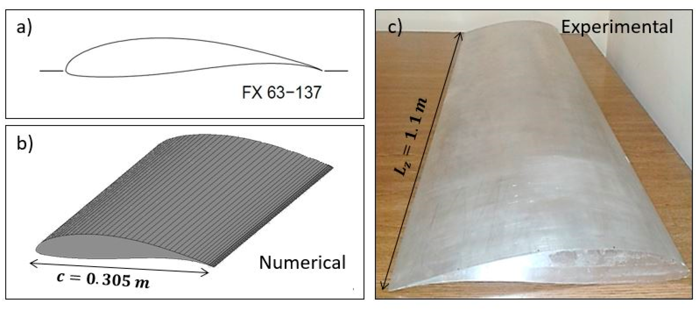
The FX 63-137 airfoil presents a maximum thickness of 13.7% of the chord, located at 30.9% of the chord length. The maximum camber, equivalent to 6% of the chord, is placed at 53.3% of the chord length. For the present study, a reference chord of 0.305 m has been considered for the numerical model (see Figure 1, left). This value has been selected to match the geometrical dimensions of a previous physical prototype made in aluminum (with a 1.1 m span, see figure right).

Intensive experimental measurements of the aerodynamic performance of this airfoil have been performed by Selig and McGranaham [13,14] at NREL (US Energy Department). It has been determined that the FX 63-137 produces a maximum lift coefficient (C_L,max) of approximately 1.7 for a wide range of Re numbers (between 100,000 and 500,000). It is also generally accepted that for Re = 100,000, the airfoil suffers the consequences of a large laminar separation bubble, especially at the lower angles of attack, with a severe fall of the lift coefficient and a quite drag force high. The situation improves for angles of attack higher than 4°, as the bubble begins to attach to the airfoil, so the lift increases, and the drag is correspondingly reduced.

Another significant characteristics of the airfoil are that (1) the FX 63-137 is susceptible for suffering a reduction of the maximum lift performance if simulated roughness is added (it is estimated to be in a drop of 0.2 in the C_L,max) and that (2) the airfoil exhibited a soft stall with little unsteadiness.

2.2. Numerical Scheme

The commercial CFD software FLUENT^® was used to solve the Navier–Stokes set of equations in an incompressible fashion, introducing an unsteady 3D viscous scheme for the finite volume method, with second-order accuracy for the temporal discretization. A bounded second-order upwind formulation has been used for the convection terms, providing a spatial accuracy with a reduced numerical diffusion, especially for complex three-dimensional flows. The diffusion terms are central-differenced and second-order accurate. On the other hand, a pressure-based solver with the SIMPLE algorithm and a Green-Gauss cell-based discretization scheme for the gradient computation has demonstrated an accurate compromise between stability and CPU time.

In addition, for the turbulence closure, an LES scheme was used to solve directly the large scales of the flow, modeling the effect of eddies smaller than the grid cell size [15]. For the subgrid-scale model, the Smagorinsky–Lilly model [16] was employed after filtering the incompressible Navier–Stokes equations (in the following, a hat denotes a subgrid average):

The continuity equation is given by:

$$\frac{\partial {\widehat{u}}_i}{\partial x_i}=0.$$

(1)

The momentum equation is given by:

$$\rho \frac{\partial {\widehat{u}}_i}{\partial t}+\rho \frac{\partial \left({\widehat{u}}_i{\widehat{u}}_j\right)}{\partial x_j}=-\frac{\partial \widehat{p}}{\partial x_i}+\mu {\nabla }^2{\widehat{u}}_i+\frac{\partial {\tau }_{ij}}{\partial x_j},$$

(2)

where ${\tau }_{ij}=-\rho \left({\widehat{u}}_i{\widehat{u}}_j-{\widehat{u}}_i{\widehat{u}}_j\right)$ is the subgrid-scale stress tensor, modeled with the Smagorinsky–Lilly closure model [16]:

$${\tau }_{ij}=2{\nu }_T{\widehat{S}}_{ij}$$

(3)

$${\nu }_T=L_S^2\left|\widehat{S}\right|={\left(C_S\widehat{\mathsf{\Delta }}\right)}^2\left|\widehat{S}\right|.$$

(4)

In Equation (4), L_S is the mixing length for subgrid scales, ν_T is the subgrid eddy viscosity, C_S is the Smagorinsky constant (0.18 in our case), $\widehat{\mathsf{\Delta }}$ is the local grid size, Sij is the resolved scale strain rate tensor and $\left|\widehat{S}\right|=\sqrt{2{\widehat{S}}_{ij}{\widehat{S}}_{ij}}$.

The Smagorinsky model is the simplest and most robust option for the subgrid-scale modeling in LES computations [17]. Despite the well-known dissipative issues of this model, especially for shock flow situations, a wide number of researchers are still relying on this SGS model for their LES computations, even in complex bladed geometries for turbomachinery (rotor/stator stages), because of its simplicity and versatility [18,19,20]. Moreover, it is recognized to still provide a good prediction of the important flow patterns and also an accurate reproduction of secondary flow features in complex flows [21].

2.3. Numerical Domain and Boundary Conditions (BCs)

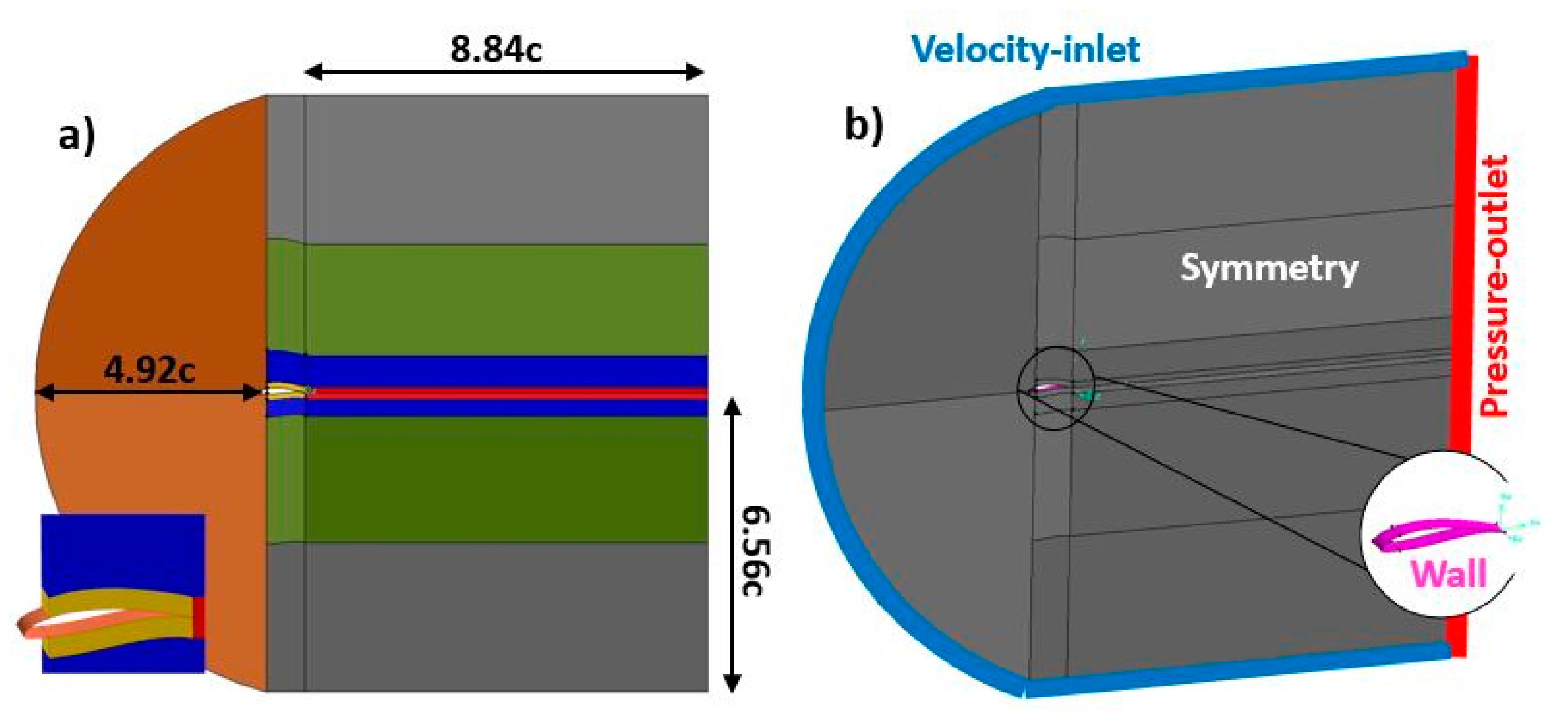
Domain sizes found in the literature in airfoil chord units c for airfoil simulation dictate typical values around 10 chord lengths for inlet distance and 20 chord lengths for outlet boundaries (see literature survey in [22]). However, it is not unusual to find reduced domains in the order of 5c upstream and just 10c downstream for LES schemes [23,24]. For the present investigation, preliminary studies [25] were performed on a 2D-RANS basis concluding the marginal effect of the boundary conditions on the flow instabilities of the wake flow. As a consequence, a reduced domain comprising 4.92c upstream from the leading edge and 8.84c downstream from the TE was finally adopted as an optimal selection for CPU costs.

Because LES simulations preclude the use of full-3D domains to resolve the three-dimensional anisotropy of the largest flow scales, it is necessary to model the spanwise direction of the airfoil with accurate precision. Since the largest scales in a boundary layer are in the order of δ, and these scales are probably also apparent in the spanwise direction [26,27], the ratio δ/L_z should at least be less than one [28], L_z being the spanwise extent of the domain. Taking into account that the boundary layer thickness obtained from the experimental measurements is about 2% of the chord [7], the spanwise dimension of the domain was set as L_z/c = 0.164, eight times larger than the maximum length scale expected to be found in the flow. Figure 2 shows a sketch with the final dimensions of the numerical domain.

Regarding the boundary conditions, a pressure outlet condition was applied in the far boundary, while the velocity-inlet condition was specified for the rest of the far-field boundaries. A moderate-to low Re number of 350,000, based on the chord length, was used at the inlet with a characteristic 0.7% turbulence intensity and an integral length scale of 0.075 m (obtained in [29] by hot wire experimental measurements). The no-slip condition was used for the airfoil walls and the symmetry condition was applied in the spanwise boundaries (top and bottom).

2.4. Computational Mesh

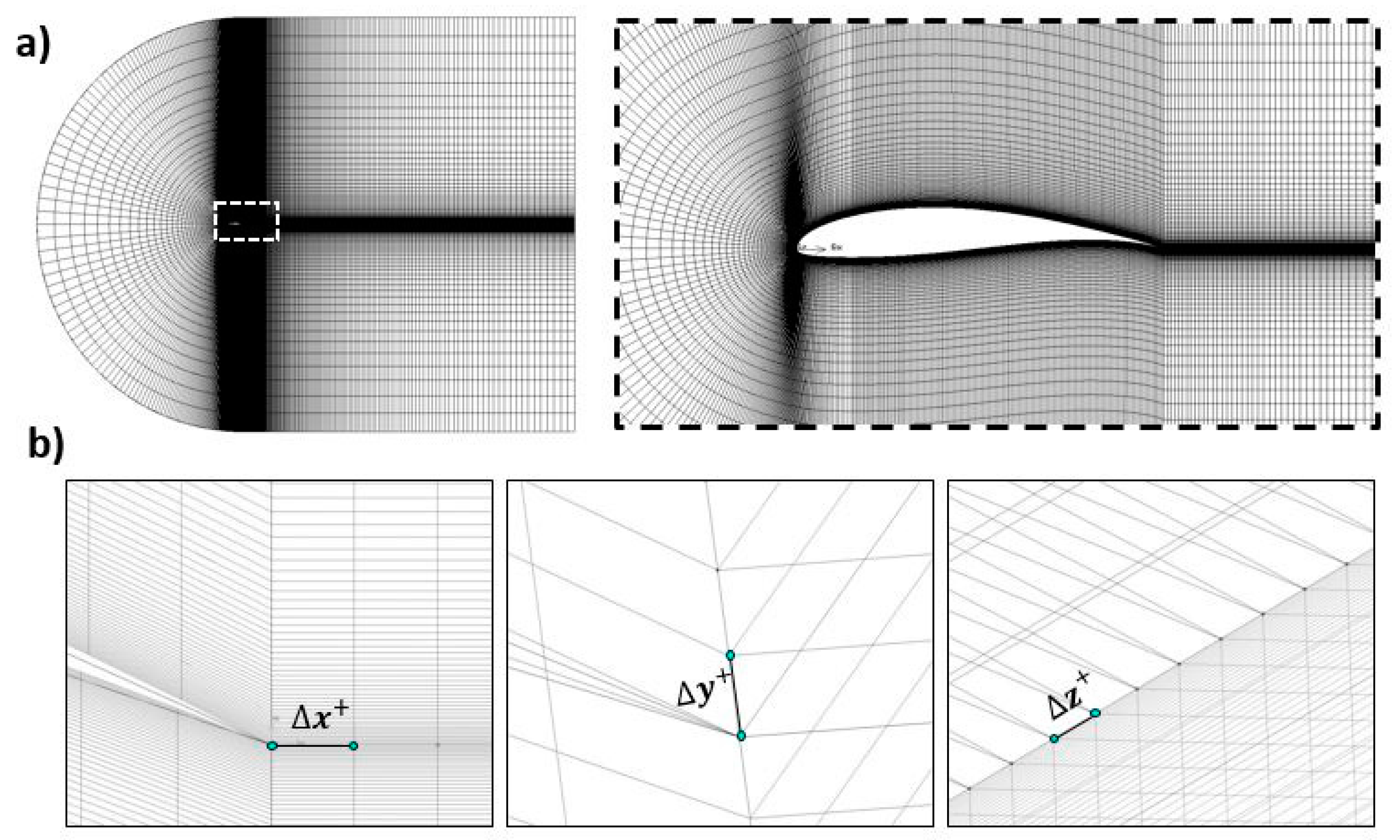
A block-structured C-mesh of 19M elements, refined at the boundary layer and TE regions, was used for the numerical simulations (Figure 3). Concerning the in-plane mesh requirements [27], recommendations are Δx⁺ = 50 to 150 and Δy+ = 1 for wall-resolved LES resolution. To ensure a good mesh resolution, stream and normal directions near the wall contours were discretized imposing Δx+ = 45 and Δy+ = 0.8. These requirements result in typical cell sizes of 0.7 mm and 0.0132 mm in the x-direction and in the y-direction, respectively. These values are also aligned with the value proposed by Pope [17], Δx+ ~ δ/10 = 0.61 mm.

Regarding the number of nodes in the spanwise direction, the guidelines proposed in references [5,17,30] were followed. Once again, in order to obtain a wall-resolved LES resolution, a dimensionless wall distance Δz+ = 10 to 40 is recommended. Taken 30 as a reasonable value, cell size was fixed to 0.4 mm, which resulted in 15 cells inside the boundary layer, quite close to the 20-cells recommendation inside the boundary layer according to Sagaut [31].

2.5. LES Modeling and Resolved Scales

Additionally, the selection of an appropriate temporal resolution to resolve the turn-out time of the resolved eddies in the LES scheme is also critical. For wall-resolved Large Eddy Simulations, the time step may be calculated as the ratio between the smallest cell size and the fluctuating velocity u’ in the airfoil walls. Assuming Δy+ ~ 1, the required time step is $\Delta t_{LES}\cong \frac{\Delta y}{u^{\prime }}=\frac{0.0132·{10}^{-3}}{0.51}=2.6\times {10}^{-5}$s, where u’ has been considered as low as 3% of the bulk velocity, according to the experimental measurements for low angles-of-attack (2.5°) in the vicinity of the airfoil wake ($u{’}^2/U^2=0.001)$. This selection is also compatible with the satisfaction of the Courant number, given the freestream velocity and the size of the cell in x-direction, corresponding to the time step finally used in these simulations, 4.05 × 10⁻⁵ s.

Not only the wall-resolved scales are important in WR-LES modeling. The typical cell size outside of the airfoil boundary layer must also ensure that at least 80% of the turbulent kinetic energy of the flow is resolved in the free-stream regions. According to [26], this leads to a typical cut-off wavenumber of the LES filter around ${\kappa }_{c}L\cong 38$, or ${\ell }_c/L\cong 0.16$, since ${\kappa }_c~2\pi /{\ell }_c$. Consequently, assuming that the integral length scale must be at least one order of magnitude lower than the chord length (L ~ 0.03 m), this leads to a requirement for the cell size around 4.8 mm. Effectively, for the 19M cells discretization over the considered volume domain (approx. 13.7 × 13.7 × 0.16·c³), the average cell size can be estimated in Δ_cell ~ (ΔV_cell)^1/3 = 3.5 mm, well-in-range with the required sizes. Moreover, the time step required to track these scales can be computed as $\Delta t_{LES}\cong \frac{1}{25}\frac{L}{U}=\frac{1}{25}\frac{0.03}{17}=7.0\times {10}^{-5}s$, following a similar rationale than URANS computations where 25 intermediate instants per cycle are usually adopted to capture those large-scale fluctuations. Note that this restriction falls within the current time-step of the modeling.

2.6. Solution Procedure, Convergence and Post-Processing

Convergence was guaranteed by monitoring the residual history of the solution, which must be dropped below 10⁻⁴ for all the resolved variables. The simulations were run for approximately 44 flow-through times, based on the freestream velocity and the airfoil chord length, until reaching a statistically steady state. This corresponds to approximately 0.8 s of throughflow time over the airfoil. Seven computers with 4-core i5 processors at 2.67 GHz and 4 Gb DDR3 RAM memory were used for the simulations, which took approximately one month to be completed and to collect the required data for post-processing.

For the identification of coherent structures comprising the movement of larger scales in the flow, the Q-criterion has been used to describe vortex-interaction phenomena. This formulation takes advantage of the nature of the big vortices arising in turbulent flows, which despite their chaotic and random nature, can be identified as “fluid regions that maintain some of their properties for a relatively large spatial and/or temporal extent” (also known as “coherent patterns”). This method [32] defines a vortex as a spatial region where the Euclidean norm of the vorticity tensor dominates that of the rate of strain:$Q=\frac{1}{2}\left({\left|{\mathsf{\Omega }}_{ij}{\mathsf{\Omega }}_{ij}\right|}^2-{\left|{\mathrm{S}}_{ij}{\mathrm{S}}_{ij}\right|}^2\right)>0$. Using this criterion, vortices in any LES computation can be detected and visualized by rendering iso-surfaces of a given Q threshold. Figure 4 shows the baseline iso-surface for Q = 5000 s⁻² in the case of 2.5° of the angle of attack.

2.7. Validation

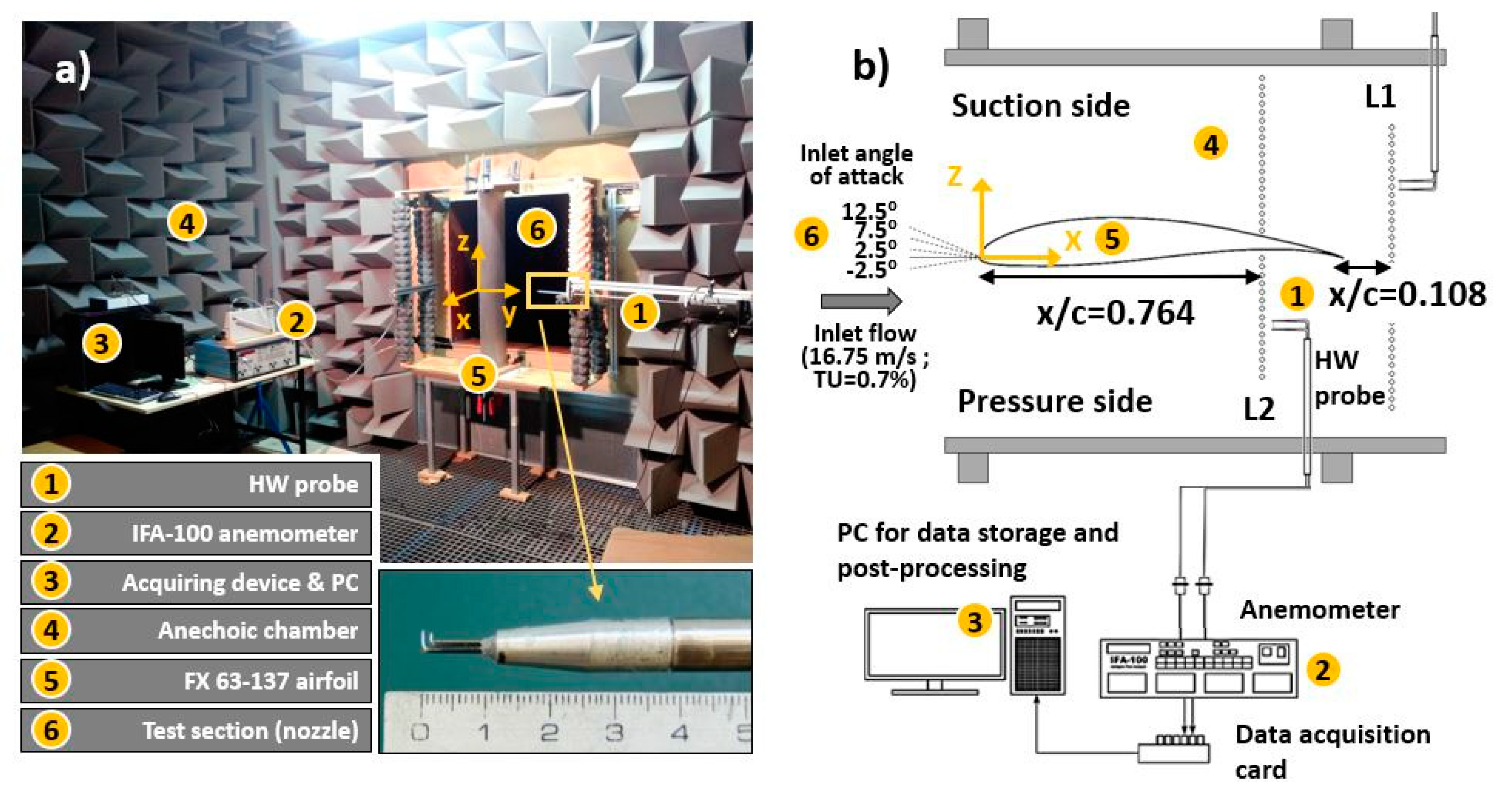
For validation purposes, an FX 63-137 airfoil model with a span of 1.1 m and a chord length of 0.305 m was aerodynamically tested in a closed-loop wind tunnel via hot-wire measurements of the flow field. Figure 5a shows a picture of the test chamber (a cross-sectional area equal to 1.0 × 1.2 m²) where the FX airfoil has been placed in a vertical arrangement. The different experimental equipment employed to complete the measurements is listed in the figure and includes (1) dual HW probe; (2) BNC connectors; (3) Inclined manometer; (4) CTA anemometer IFA-100; (5) Acquiring card; (6) PC; (7) Anechoic chamber and (8) FX 63-137 airfoil. More details about the measuring devices can be found in [7,25].

The measurements were performed at 10 kHz over 25 s for every position. A convergence study of the mean velocity was made by increasing the number of samples for each measurement point until the results no longer differed. Measurements were made by sweeping two rakes at different streamwise locations: L1, in the airfoil wake (x = 1.108c) and L2, at around 75% of the airfoil chord (x = 0.764c). This last location was chosen because it is a representative position of the high airfoil curvature. Both positions may be seen in Figure 5-right.

Wake (L1) and Airfoil (L2) will be used to refer to these positions. In each rake, different positions were measured and for every position, a sample of 250,000 point values was obtained with hot-wire anemometry (see Figure 5). The velocity profile for every angle was built through the time average of the point values in every position of the rake. The airfoil was placed at four different incidence angles: -2.5°, 2.5°, 7.5° and 12.5°, none close to stall, and at a 350,000 Re number.

From these measurements, instantaneous values of in-place velocity, velocity angle, turbulence intensities and integral length scales can be obtained for different angles of attack. Hence, all these experimental results will be later compared to the numerical results, so the computations via LES modeling may be positively validated.

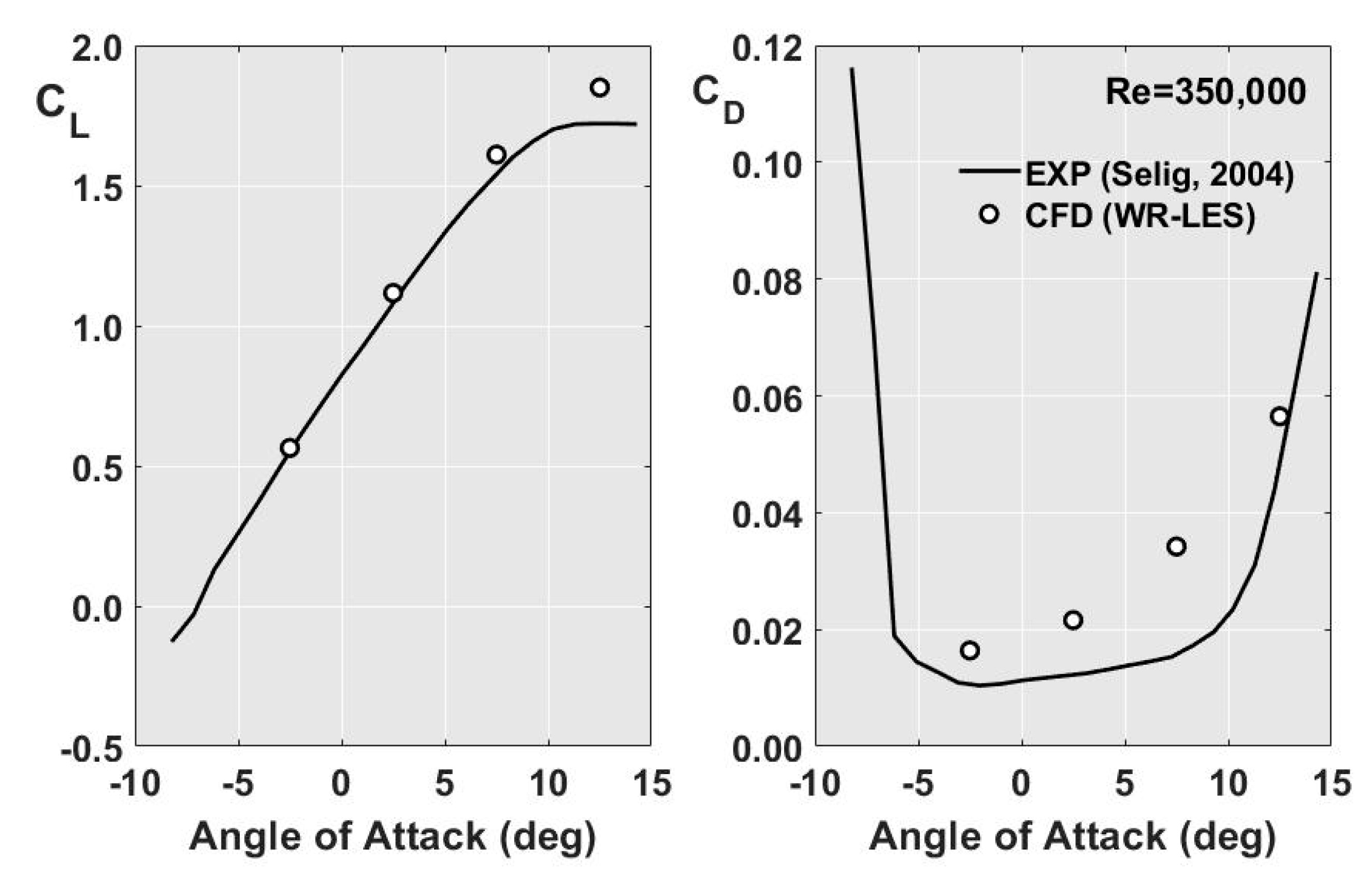
In addition, the lift and drag coefficients obtained with the present LES simulation have been compared with the experimental results provided by Selig and McGranaham [14] for a smooth FX 63-137 airfoil, as shown in Figure 6. The solid black lines provide the experimental results measured for Re = 350,000 in the UIUC low-speed subsonic wind tunnel (NREL), at free-stream turbulence levels below 0.1%. The white dots correspond to the present CFD results after time-averaging, obtained when both aerodynamic coefficients are stabilized (typically, after 25–30 flow-through times). The lift coefficient is perfectly matched in the unstalled region by the computations, with maximum deviations in the range of just 2.5%. Only at 12.5°, the LES computations and the experimental results show a slight discrepancy. In the case of the drag coefficient, the differences are remarkable for all the range of angles of attack simulated, being the C_D always higher in the simulations. This can be attributed to the difference in the free-stream turbulence level between the NREL wind tunnel (roughly 0.1%) and the turbulence intensity imposed in the LES modeling (0.7%, in resemblance to the wind tunnel shown in Figure 5). In particular, the effect of the free-stream turbulence on the aerodynamic performance of airfoils can be drastic when they are operated at low turbulence levels. Huang and Lee [33] have reported severe drag increments with the increase in freestream turbulence intensity, especially if the value is below 0.45%, which is in correspondence to the present database. The artificial overestimation of the drag coefficient in the computations can thus be perfectly associated with the high free-stream turbulence level employed in the model. Another source of uncertainty can be identified in the momentum method employed by Selig to estimate the drag force over the airfoils indirectly. Depending on the position of the traverse hot-wire that it is measuring the velocity profiles at the wake sections, the two-dimensional theory may lead to significant errors in the determination of the drag coefficient. Note that for the C_L, Selig and McGranaham do employ a beam balance to measure the lift force directly.

3. Results and Discussion

This section, presenting the most remarkable results of the simulation, has been divided in five different subsections. Section 3.1 and Section 3.2 include results from the velocity fields, that are compared with HW measurements for validation purposes. Following, the other subsections are focused on a detailed description of the boundary layer characteristics over the airfoil.

3.1. Velocity Components and Reynolds Stresses

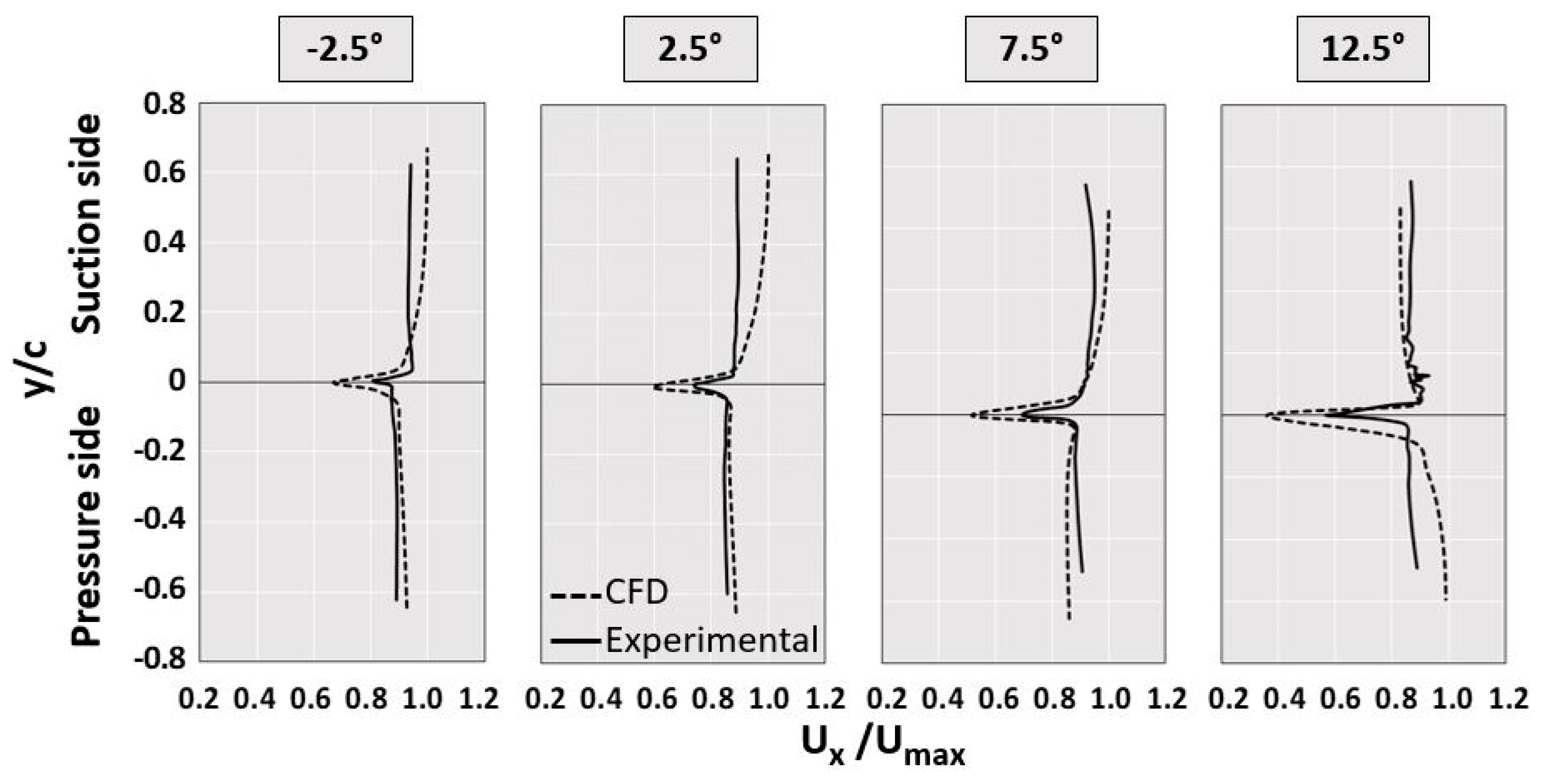
The normal-to-airfoil distribution of the streamwise velocity (x-coordinate) is shown at L1, for the angles of attack tested, in Figure 7. Both experimental and numerical values, normalized by the maximum velocity, are compared for validation purposes, showing a good agreement. Particularly, the wake width is perfectly predicted by the LES modeling, though its deficit is slightly overestimated. This is due to a geometrical penalty of the experimental airfoil in the trailing edge, associated with mechanical deviations. As a consequence, the flow is longer attached to the airfoil in the numerics, resulting in a modeled wake deeper than the real one. The largest discrepancies between experimental and numerical results are found at 12.5°, when the flow is more detached and the three-dimensional effects of the trailing edge are more evident.

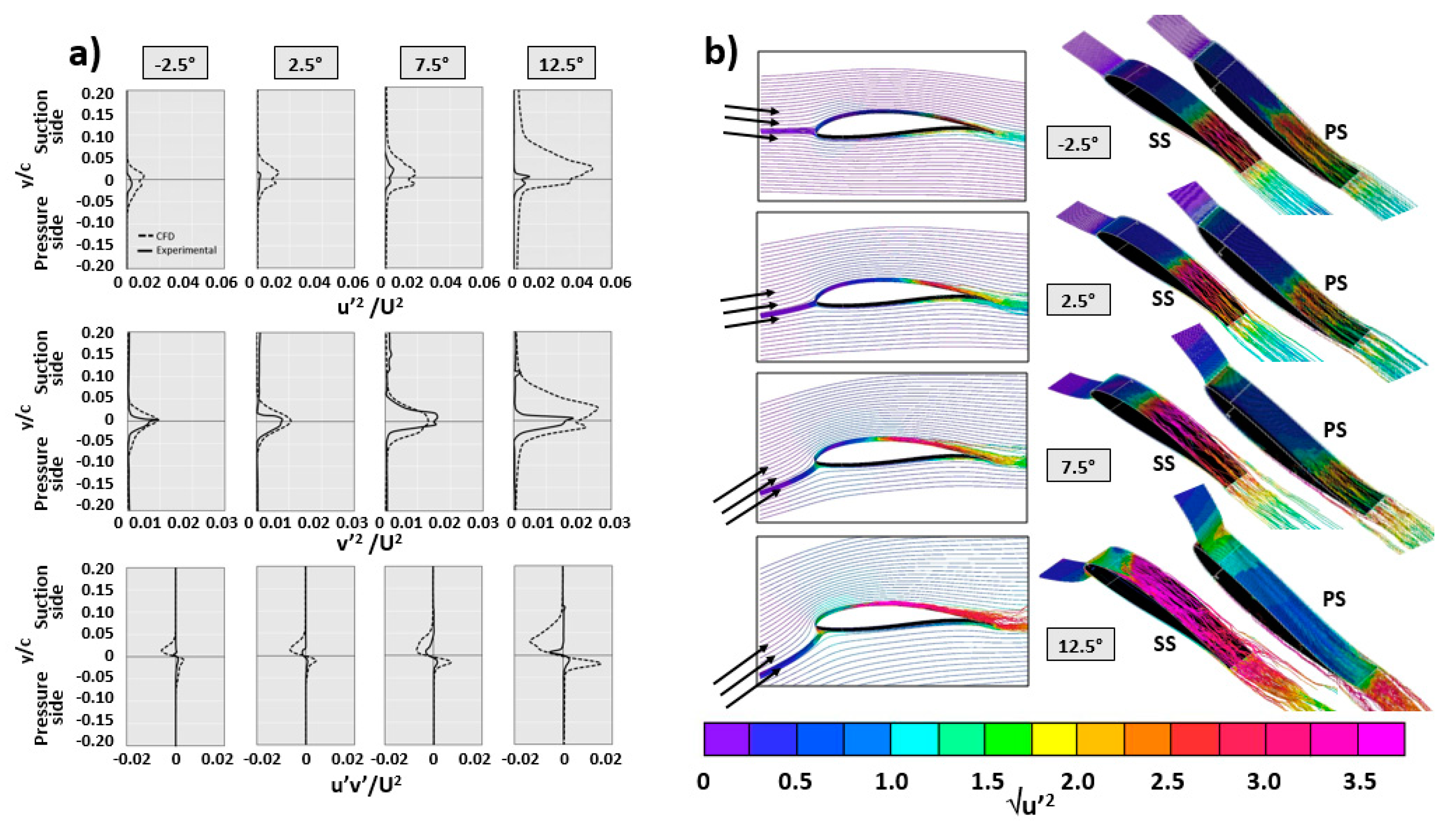
Another interesting comparison comes from the different distributions of the Reynolds stresses in the wake region, obtained from the time-averaging of the velocity fluctuations. Figure 8a compares numerical and experimental results including longitudinal $\left(u{’}^2/U^2\right)$, transversal $\left(v{’}^2/U^2\right)$ and crossed $\left(u’v’/U^2\right)$ components of the Reynolds stresses for all the tested angles of attack. In general, simulation results present a similar trend when compared to experimental measurements, exhibiting a double-peak pattern in the longitudinal component with a local minimum that corresponds to the minimum wake velocity. On the other hand, the magnitude of the numerical results for this component shows significant differences, especially at higher angles of attack. In the case of the transversal component, a one single peak characteristic for reduced angles of attack is observed, which is progressively evolving into a double-peak distribution as the angle of attack increases. Finally, it is significant for the crossed component how the sign is switched in the wake center at the minimum velocity, being more evident for positive angles of attack with a positive peak in the pressure side and a negative peak in the suction side. Additionally, it is remarkable that the suction side contributes more than the suction side to the Reynolds stresses in the wake fluid. This is due to the reinforcement of the instabilities in the shear layer of the suction side, associated with the detached flow conditions as the angle of attack increases.

Complementarily, Figure 8b reveals the flow streamlines along the airfoil, computed by the numerical simulations for the different angles of attack of the incoming flow. Note that the streamlines have been colored by the local intensity of the turbulent fluctuations of the streamwise velocity. As expected, in the case of a low angle of attack, the flow is smoothly attached to the airfoil geometry (see for instance the suction side at 2.5°). However, for higher incidence angles, the streamlines become unstable, following irregular trajectories like in the case of the suction side at 12.5°. Besides, the longitudinal fluctuations tend to be more concentrated towards the leading edge in the suction side as the angle of attack is enlarged. The opposite trend is observed in the pressure side, with the largest area of instabilities in the case of −2.5°. (the negative angles of attack). This behavior, directly related to the boundary layer, is explained in more detail in the following sections.

3.2. Integral Length Scale

Figure 9a shows the normal-to-airfoil distributions of the integral length scale (ILS), comparing both experimental and numerical results. The ILS is a metric to assign a characteristic spatial dimension to the turbulent structures of the flow; in particular, to provide the average size of the largest eddies (vortices) in the flow. The integral scale is calculated from the autocorrelation of the turbulent fluctuations of the instantaneous velocity field according to:

$$ILS=U{{\displaystyle \int }}_0^{\infty }\frac{\overline{u^{\prime }\left(t\right)·u^{\prime }\left(t+\tau \right)}}{\overline{u{’}^2}}d\tau ,$$

(5)

where the overbar denotes the time-averaging value, and τ is the time lag that is used to construct the autocorrelation function. This expression supposes the validity of Taylor’s hypothesis (the average eddy size lies through the correlation of two velocity signals). Obviously, the time lag depends directly on the data sampling rate, so an average eddy of a wave number larger than the sampling rate cannot be measured.

Inside the instability regions, eddies tend to be of a low scale; but in the non-perturbed regions in the middle of the test section, they are large with a significant uniformity. Besides, three different zones are identified along the transversal coordinate: (1) the instability zone related to the wake or the boundary layer; (2) the transition region and (3) the external zone for the bulk flow. Generally speaking, major discrepancies between experimental and numerical results are found in the transition region due to the large number of all-size vortices generated.

Numerical results provide a remarkable agreement with the experimental data in case of angles of attack of −2.5°, 2.5° and 7.5°. (at 12.5°, the numerical values differ significantly with the experiments). As the angle of attack is increased, the typical size of the turbulent eddies is also enlarged, especially in the external, free region of the suction side. Anyway, the highest differences are found at 12.5°, especially in the pressure side of the airfoil as well as in the transition region of the suction side. Additionally, the maps obtained from the numerical results (Figure 9b) confirm this trend (underestimation in the numerical results) in the case of the highest angle of attack because the numerical model should generate large-scale vortices, higher than any other angle of attack.

Despite the evident differences observed in both subsections 3.1° and 3.2° for the case of 12.5°, the results obtained from the LES simulations for the rest of the angles of attack provide very similar results, with overall trends and magnitudes in agreement with the experimental data. This leads to assume that the wall-resolved model is reproducing with accurate fidelity the real flow behavior around the Wortmann airfoil. Following, more numerical results are presented to give more insight into the physical phenomena.

3.3. Turbulent Kinetic Energy (TKE)

The turbulent kinetic energy (TKE) can be obtained from the segregation of the instantaneous velocities and their time-averaged values. However, in LES simulations, there is residual kinetic energy modeled below the grid filter, that should have to be accounted for to provide a more precise value of the turbulent fluctuations.

The resolved turbulent kinetic energy, defined from the addition of the components of the main diagonal of the Reynolds Stress Tensor at every time step, provides a collection of instantaneous values. From the collected data of the LES simulation, and after time-averaging, it has been obtained for the different angles of attack according to:

$$k_{res}=\frac{1}{2}\left({\left(u-\overline{u}\right)}^2+{\left(v-\overline{v}\right)}^2+{\left(w-\overline{w}\right)}^2\right).$$

(6)

It is important to recall that this formulation gives only the resolved part of the whole turbulent energy budget. A complete estimation of the TKE requires the summation of the additional sub-grid TKE. However, the sub-grid component is quite marginal when a rough estimation of the resolved energy is around 80% (or higher). Nevertheless, it is necessary to check if it is acceptable to consider the resolved part as the major contributor, obviating the sub-grid scales. To contrast this assumption, the comparison of both resolved and sub-grid components is presented below, using the sub-grid turbulent viscosity as the primary contributor for the computation of the subgrid scales according to the model Equations (1)–(4). After some dimensional considerations [34], the sub-grid TKE can be calculated from:

$$k_{\mathit{sgs}}\cong {\nu }_T^2/{\left(C_S\widehat{\mathsf{\Delta }}\right)}^2$$

(7)

where Δ = (ΔxΔyΔz)^1/3 stands for the averaged size of a computational cell and C_S is the Smagorinsky constant. In a porcentual basis, the residual turbulent kinetic energy is computed as:

$$k_r[\%]=\frac{k_{\mathit{sgs}}}{k_{\mathrm{res}}+k_{\mathit{sgs}}}·100.$$

(8)

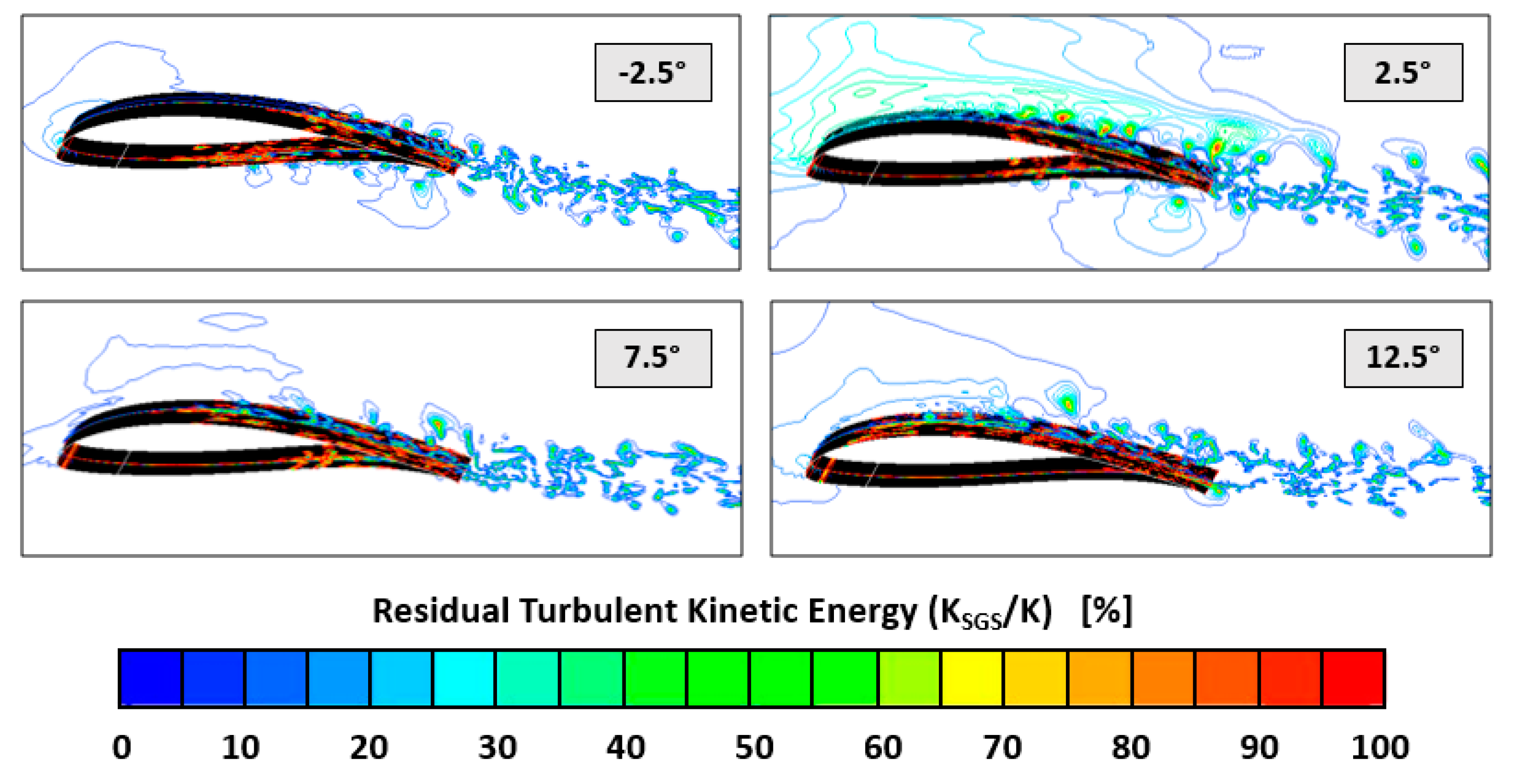
Figure 10 represents the residual turbulent kinetic energy for all the tested angles of attack. Regions with higher values correspond to locations where a major spatial resolution is needed to be resolved (and not modeled) by the LES scheme. In particular, these regions are associated with the shear layers of the wake fluid, especially in the suction side of the airfoil in case of detached flow. These instabilities lead to the arising of intermittent rolling vortices which would require even finer meshes in the case of 2.5°. angle of attack. Complementarily,

Table 1. Volume-averaged values of residual turbulent kinetic energy (TKE) in the domain at different angles of attack.

Angle of Attack	−2.5°	2.5°	7.5°	12.5°
$k_r^{\left(LES\right)}$ (Numerical)	2.03%	7.49%	1.82%	1.16%

provides the volume-averaged value of the residual kinetic energy for the whole domain. The summarized data reveals that the 2.5°. situation is the one with the highest levels (roughly a 7.5%), although it is also clearly manifested that the residual TKE is far below the 20% threshold assumed during the mesh design. The results from this subsection determine the validity of the mesh proposed, with very low and assumable modeled TKE, for all the tested angles of attack.

3.4. Description of the Boundary Layer (BL)

As described in the Introduction section, trailing edge (TE) noise is considered one of the major noise generation mechanisms for rotor blades of wind turbines. TE noise is due to the scattering of the vortical disturbances in the boundary layer into acoustic waves at the airfoil TE. In order to provide an insight into this noise generation mechanism, this subsection presents a detailed analysis of the boundary layer in the FX 63-137 airfoil, showing the numerical results of the LES modeling and making a comparison with simple estimations given by the XFOIL software. XFOIL is a useful and well-known code [35], based on the panel’s method for potential flow and combined with an integral formulation of the BL. It was specifically developed for a rapid prediction of an airfoil behavior at low Re numbers. It can provide the pressure distribution in the viscous flow region, as well as compute the influence of the flow separation in the airfoil TE or the effect of a laminar separation bubble. Hence, the XFOIL code provides a very complete description of those variables having an impact on the final characteristics of the airfoil BL. In addition, both lift and drag coefficients, pressure distributions and velocities in the layer, momentum and displacement thicknesses can be estimated, so the BL type developed on the airfoil can be identified.

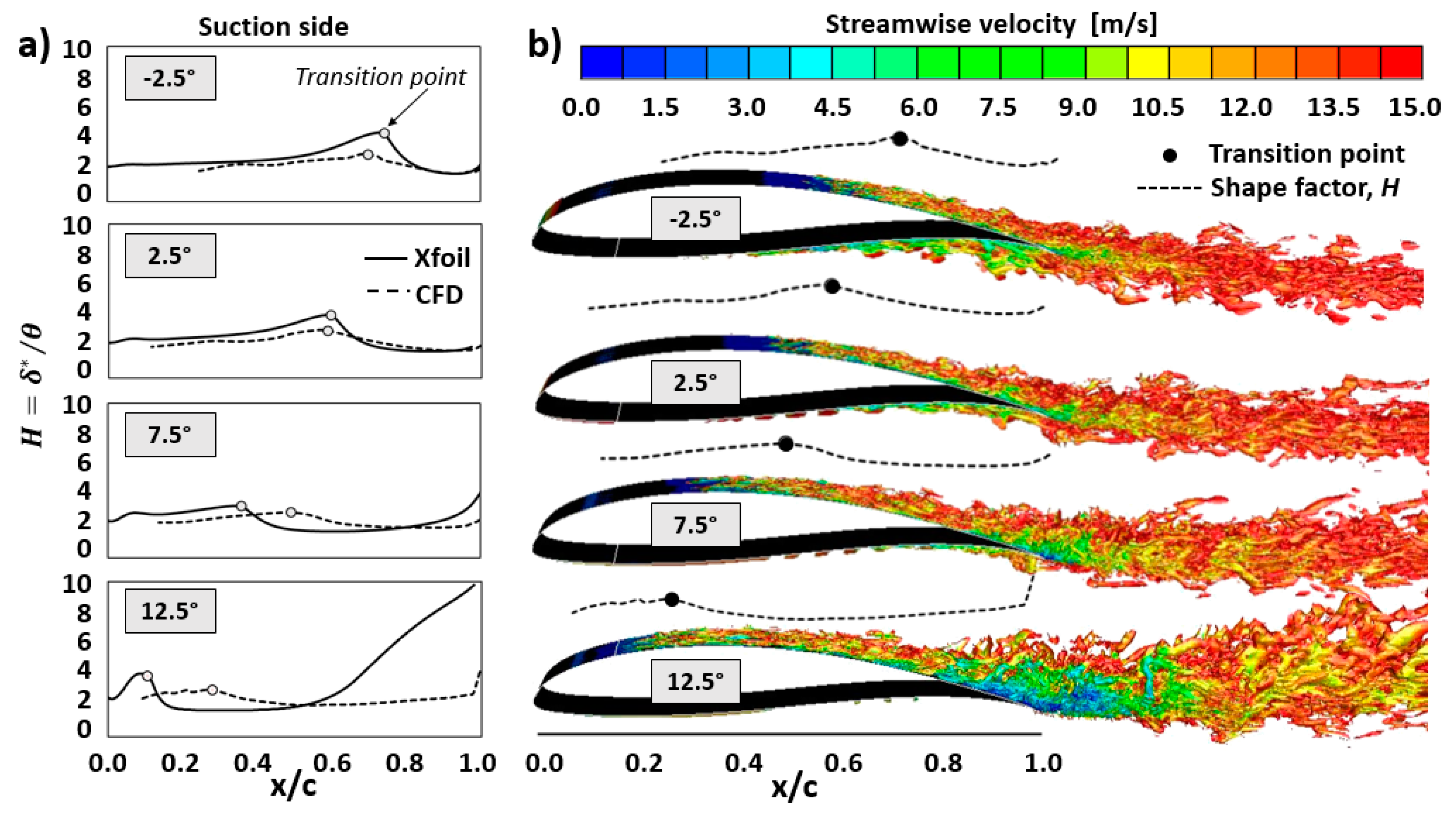
In a BL, the shape factor H, which is defined as the ratio between the displacement thickness, δ^*, and the momentum thickness, θ, indicates the different phases for the establishment of a boundary layer. The higher the value of H, the stronger the adverse pressure gradient. A high adverse pressure gradient can greatly reduce the Re number at which transition into turbulence may occur. Figure 11a shows the streamwise distribution of the shape factor in the suction side BL as a function of the angle of attack, comparing XFOIL estimations (solid lines) with LES computations (dashed lines). Both methods provide similar trends, with the largest discrepancies in the case of 12.5°. In that situation, XFOIL predicts a massive separation in the airfoil TE, while LES results confirm the separation but significantly smoother.

Based on the shape factor value, it can be judged if the BL is laminar or fully-turbulent. Typically, a shape factor around 1.8 is characteristic of a turbulent BL, while values around 2.4 correspond to a laminar BL. All the plots in the figure indicate the initial laminar behavior of the suction BL for all the angles of attack analyzed. Following, the transition to turbulent BL is experienced at some intermediate point, which is progressively displaced towards the LE as the angle of attack increases. Precisely, the white dots in the plots represent the location where both methods predict the transition point, identified as the local maxima of the shape factor along the airfoil’s suction side [36].

Mayle [37] describes four different transition mechanism in boundary layers: (1) A natural transition takes place when the process is set off due to the arising of small instabilities in the BL; (2) When the freestream turbulence level is high, the turbulent flow is abruptly developed, leading to the establishment of a rapid transition; (3) In the case of separation of the laminar BL, followed by reattachment, a separation bubble is generated and the process is called transition of detached flow; (4) Finally, when an incipient BL in transition undergoes an intense favorable pressure gradient so it turns into laminar, the process is called relaminarization transition.

In the present case, as shown in Figure 11a, the maximum values of the shape factor in the transition region of the BL are not excessively high, so the transition can be defined as natural, without suffering detached flow prior to separation or even laminar separation. Only in the case of 12.5°, the transition is corresponding to detached flow, since high values of the shape factor are observed close to the TE in the suction side of the airfoil. Although both XFOIL and LES results are similar, it is evident that the detached prediction is much more abrupt for the XFOIL predictions. This is because the separation flow estimation is based on the prediction of the transition point of the BL, which is always significantly displaced towards the LE in the XFOIL results. Precisely, when the BL is thicker and more instabilities arise (suction sides at 7.5° and 12.5°), it is when higher discrepancies in the transition point determination are found.

Complementarily, the Q-criterion is also employed to visualize the characteristics of the BL in the LES computations, Figure 11b, as a function of the angle of attack. For a higher readability, the computed shape factor and the transition points have been also re-plotted close to the isosurfaces, which represent a typical value of Q = 50,000 s⁻², colored by the instantaneous streamwise velocity. This indicator, as defined in Section 2.6, allows us to know the overall vorticity levels and the size of the turbulent structure of the flow [38].

Rotational instabilities of the flow can be tracked using the Q-criterion along the airfoil. In particular, for both suction and pressure sides, this indicator reveals the generation of Tollmien–Schlichting (T-S) waves, which are known to be an important mechanism for the generation of noise in airfoils. When a small instability arises in the laminar BL, it evolves generating vortices that eventually break-up, interacting with other adjacent instabilities and thus contributing to set off the natural transition of the BL into a turbulent regime. The T-S waves are a usual mechanism that participates in the transition from laminar to turbulent flow and with an evolution composed by several stages. Firstly, the momentum thickness reaches a critical value, so the BL becomes susceptible to small flow perturbations that allow the arising of 2D wave instabilities. In a second stage, these waves are enlarged, evolving into three-dimensional instabilities that finally lead to the appearance of vortical fluctuations. In a final stage, these 3D vortices are collided downstream, forming coherent turbulent structures that compose the fully-developed turbulent BL.

The diffraction of the T-S instabilities at the trailing edge generates acoustic waves that are propagated into the far-field, being a significant contribution to the total noise level radiated by the airfoil. In particular, they are found as a tonal component in the noise spectrum of the flow [1]. However, if these perturbations are diffused into a turbulent boundary layer prior to the airfoil trailing edge, this tonal noise is removed. Figure 11b reveals those T-S waves that are generated in both suction and pressure sides and that are more evident in the cases of 2.5° and 7.5°. This suggests that those intermediate angles of attack are the ones with a more gradual and controlled transition from laminar to turbulent BL. Note that these waves are not reaching the airfoil TE in any of the angles of attack studied, so they are not introducing tonal contributions to the noise emission propagated to the far-field. This finding has been already reported in the open literature by the authors in previous works [7].

3.5. Pressure Coefficient

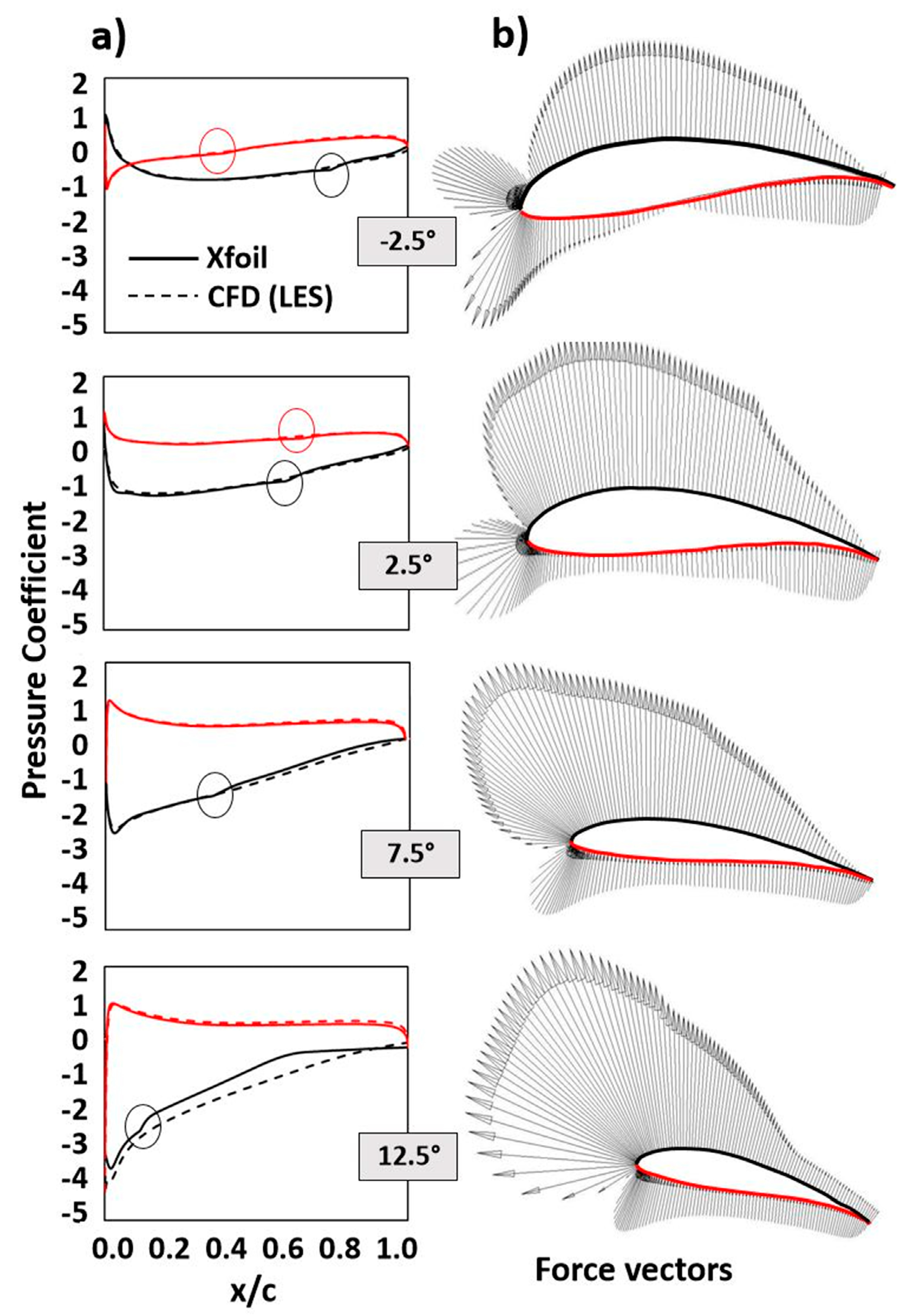
To conclude the results section, the pressure coefficient on the airfoils at different angles of attack is shown in Figure 12a for both XFOIL (solid lines) and LES (dashed lines) methodologies. The coefficient is defined as the difference between the local and freestream static pressure, normalized by the incoming dynamic pressure. Red lines correspond to the pressure side while black lines identify the suction side.

In this case, it is really remarkable the good agreement found between both numerical models. Only in the suction side at 12.5° there is a clear lack of correspondence, as previously reported for the shape factor. At all the angles of attack, the transition is more evident in the suction side, as it is identified with circle marks in the plots. It is noticeable how the distribution of the pressure coefficient on the suction side changes severely with the angle of attack. Conversely, in the pressure side, the transition point is practically imperceptible at 7.5° and 12.5°, since it has been displaced towards the airfoil TE. In summary, as the angle of attack increases the transition point on the suction side progressively approaches the LE, while on the pressure side the transition point moves towards the TE.

Due to its high curvature, the FX 63-137 airfoil provides a remarkable lift, with a C_L,max around 1.7 for a Re number of 350,000 and angles of attack between 14°–16°. It is also known that this profile generates a large bubble of laminar separation when the Re number is 100,000. This bubble probably does not reattach to the airfoil for small angles of attack, but it certainly reaches the downstream wake, as it is inferred from the behavior of the lift and drag curves corresponding to Re = 10⁵ [13,14]. However, no laminar separation bubbles are generated at low angles of attack for Re = 3.5 × 10⁵, as it has been also confirmed from the present numerical computations using a high-fidelity, wall-resolved LES modeling.

4. Conclusions

A wall-resolved LES model of the flow around a typical wind turbine airfoil has been developed and resolved, in order to describe the main features of the turbulent structures and the boundary layer. The numerical results obtained have been validated with hot wire measurements in a wind tunnel. Despite some differences observed and explained for the higher angle of attack, the results obtained from the LES simulations for the best angles of attack have shown overall trends and magnitudes in agreement with the experimental data.

The detailed description of the development of the boundary layer over the airfoil provides an insight into the main noise generation mechanism in wind turbines, which is known to be the scattering of the vortical disturbances in the boundary layer into acoustic waves at the airfoil trailing edge. In this case, 2D wave instabilities are observed in both suction and pressure sides, but these perturbations are diffused into a turbulent boundary layer prior to the airfoil trailing edge, so tonal noise components are not expected in the far field noise propagation.

The detailed description of this experimentally validated wall-resolved LES model can be useful as a guide to another modeling works of similar features. The results obtained can also be used as input data for the prediction of noise propagation to the far-field using a hybrid aeroacoustic model.

References

1. Arcondoulis, A.; Doolan, C.; Zander, A.; Brooks, L. A review of trailing edge noise generated by airfoils at low to moderate Reynolds number. Acoust. Aust. 2010, 38, 129–133. [Google Scholar]
2. Oerlemans, S.; Fisher, M.; Maeder, T.; Kögler, K. Reduction of wind turbine noise using optimized airfoils and trailing-edge serrations. AIAA J. 2009, 47, 1470–1481. [Google Scholar] [CrossRef]
3. Blake, W. Mechanics of Flow Induced Sound and Vibration; Academic Press: New York, NY, USA, 1986. [Google Scholar]
4. Wagner, S.; Bareiss, R.; Guidati, G. Wind Turbine Noise; Springer: Berlin, Germany, 1996. [Google Scholar]
5. Tucker, P. Unsteady Computational Fluid Dynamics in Aeronautics; Springer: Berlin, Germany, 2014. [Google Scholar]
6. Lighthill, M. On sound generated aerodynamically. Part I: General theory. Proc. R. Soc. Lond. 1952, 211, 564–587. [Google Scholar]
7. Solís-Gallego, I.; Meana-Fernández, A.; Fernández Oro, J.M.; Argüelles Díaz, K.M.; Velarde-Suarez, S. LES-based numerical prediction of the trailing edge noise in a small wind turbine airfoil at different angles of attack. Renew. Energy 2018, 120, 241–254. [Google Scholar] [CrossRef]
8. Curle, N. The influence of solid boundaries upon aerodynamic sound. Proc. R. Soc. Lond. 1955, 231, 505–514. [Google Scholar]
9. Ffowcs Williams, J.; Hall, L. Aerodynamic sound generation by turbulent flow in the vicinity of a scattering half plane. J. Fluid Mech. 1970, 40, 657–670. [Google Scholar] [CrossRef]
10. Roache, P. Verification and Validation in Computational Science and Engineering; Hermosa Publishers: Alburquerque, NM, USA, 1998. [Google Scholar]
11. Althaus, D.; Wortmann, F. Stuttgarter Profilkatalog I; Institut für Aerodynamik, Friedr. Vieweg & Sohn: Braunschweig/Wiesbaden, Germany, 1981. [Google Scholar]
12. Man-powered planes get a new lift. In Popular Science; Popular Science Publishing Co.: New York, NY, USA, 1972.
13. Selig, M.S.; McGranahan, B.D. Wind tunnel aerodynamic tests of six airfoils for use on small wind turbines. In Technical Report, NREL/SR-500-34515; National Renewable Energy Laboratory, U.S. Department of Energy: Golden, CO, USA, 2003. [Google Scholar]
14. Selig, M.S.; McGranahan, B.D. Wind tunnel aerodynamic tests of six airfoils for use on small wind turbines. J. Sol. Energy Eng. 2004, 126, 986–1001. [Google Scholar] [CrossRef]
15. Piomelli, U. Large Eddy Simulation and Related Techniques; Lecture Series 2006-04; Von Karman Institute for Fluid Dynamics: Brussels, Belgium, 2006. [Google Scholar]
16. Smagorinsky, J. General circulation experiments with the primitive equations. I. The basic experiment. Mon. Weather Rev. 1963, 91, 99–164. [Google Scholar] [CrossRef]
17. Pope, S.B. Turbulent Flows; Cambridge University Press: London, UK, 2000. [Google Scholar]
18. Wang, G.; Duchaine, F.; Papadogiannis, D.; Duran, I.; Moreau, S.; Gicquel, L. An overset grid method for large eddy simulation of turbomachinery stages. J. Comput. Phys. 2014, 274, 333–355. [Google Scholar] [CrossRef]
19. Zauner, M.; Sandham, N.; Wheeler, A.; Sandberg, R.D. Linear stability prediction of vortex structures on high pressure turbine blades. Int. J. Turbomach. Propuls. Power. 2017, 2, 8. [Google Scholar] [CrossRef] [Green Version]
20. McMullan, W.; Page, G. Towards large eddy simulation of gas turbine compressors. Prog. Aerosp. Sci. 2012, 52, 30–47. [Google Scholar] [CrossRef] [Green Version]
21. Papadogiannis, D.; Duchaine, F.; Gicquel, L.; Wang, G.; Moreau, S. Effects of subgrid scale modeling on the deterministic and stochastic turbulent energetic distribution in large-eddy simulations of a high-pressure turbine stage. J. Turbomach. 2016, 138, 091005. [Google Scholar] [CrossRef]
22. Meana-Fernández, A.; Fernández Oro, J.M.; Argüelles Díaz, K.M.; Velarde-Suárez, S. Turbulence-model comparison for aerodynamic-performance prediction of a typical vertical-axis wind-turbine airfoil. Energies 2019, 12, 488. [Google Scholar] [CrossRef] [Green Version]
23. Cao, H. Aerodynamics Analysis of Small Horizontal Axis Wind Turbine Blades by Using 2D and 3D CFD Modelling. Master’s Thesis, University of Central Lancashire, Preston, UK, 2011. [Google Scholar]
24. Mendez, B.; Muñoz, A.; Munduate, X. Study of distributed roughness effect over wind turbine airfoils performance using CFD. In Proceedings of the 33rd Wind Energy Symposium, Kissimmee, FL, USA, 5–9 January 2015. [Google Scholar]
25. Solis-Gallego, I. Caracterización Del Comportamiento Aeroacústico De Perfiles De Turbinas Eólicas En Flujo Turbulento. Master’s Thesis, University of Oviedo, Asturias, Spain, 2017. (In Spanish). [Google Scholar]
26. Tucker, P. Computation of unsteady turbomachinery flows: Part 2—LES and hybrids. Prog. Aerosp. Sci. 2011, 47, 546–569. [Google Scholar] [CrossRef]
27. Dahlström, S.; Davidson, L. Large eddy simulation of the flow around an aerospatiale A-aerofoil. In Proceedings of the European Congress on Computational Methods in Applied Sciences and Engineering ECCOMAS 2000, Barcelona, Spain, 1–3 September 2000; pp. 1–20. [Google Scholar]
28. Davidson, L.; Dahlström, S. Hybrid LES-RANS: An approach to make LES applicable at high Reynolds number. Int. J. Comput. Fluid Dyn. 2005, 19, 415–427. [Google Scholar] [CrossRef]
29. Lastra, M.; Fernández Oro, J.M.; Galdo Vega, M.; Blanco Marigorta, E.; Santolaria Morros, C. Novel design and experimental validation of a contraction nozzle for aerodynamic measurements in a subsonic wind tunnel. J. Wind Eng. Ind. Aerodyn. 2013, 118, 35–43. [Google Scholar] [CrossRef]
30. Chapman, D. Computational aerodynamics development and outlook. AIAA J. 1979, 17, 1293–1313. [Google Scholar] [CrossRef]
31. Sagaut, P. Large Eddy Simulation for Incompressible Flows; Springer: Berlin, Germany, 2006. [Google Scholar]
32. Haller, G. An objective definition of a vortex. J. Fluid Mech. 2005, 525, 1–26. [Google Scholar] [CrossRef] [Green Version]
33. Huang, R.F.; Lee, H.W. Effects of freestream turbulence on wing-surface flow and aerodynamic performance. J. Aircr. 1999, 36, 965–972. [Google Scholar] [CrossRef]
34. Comte-Bellot, G. Hot-wire and hot-film anemometers. In Measurement of Unsteady Fluid Dynamic Phenomena; Richards, B.E., Ed.; Hemisphere: Washington, DC, USA, 1977; pp. 123–162. [Google Scholar]
35. Drela, M. XFOIL: An analysis and design system for low reynolds number airfoils. In Lecture Notes in Engineering; Mueller, T.J., Ed.; Springer: New York, NY, USA, 1989; Volume 54. [Google Scholar]
36. Cebeci, T.; Mosinskis, G.; Smith, M. Calculation of separation points in incompressible turbulent flows. J. Aircr. 1972, 9, 618–624. [Google Scholar] [CrossRef]
37. Mayle, R. The 1991 IGTI Scholar Lecture: The role of laminar-turbulent transition in gas turbine engines. J. Turbomach. 1991, 113, 509–537. [Google Scholar] [CrossRef]
38. Winkler, J.; Carolus, T.; Moreau, S. Airfoil trailing edge blowing: Broadband noise prediction from large eddy simulation. In Proceedings of the 15th AIAA/CEAS Aeroacoustics Conference (30th AIAA Aeroacoustics Conference), Miami, FL, USA, 11–13 May 2009. [Google Scholar]
Figure 1. Airfoil FX 63-137. (a) 2D section. (b) 3D numerical blade. (c) Experimental model.
Jmse 08 00212 g001
Figure 2. Numerical domain. (a) Upstream and downstream extension. (b) Boundary conditions.
Jmse 08 00212 g002
Figure 3. (a) Computational mesh. (b) Minimum cell sizes in the different coordinates.
Jmse 08 00212 g003
Figure 4. Example of vortex identification using the Q-criterion for a 2.5° angle of attack.
Jmse 08 00212 g004
Figure 5. (a) Experimental setup for hot-wire measurements. (b) Sketch of the measuring database.
Jmse 08 00212 g005
Figure 6. Comparison of experimental (the data from Selig and McGranaham [13]) and numerical aerodynamic coefficients at Re = 350,000.
Jmse 08 00212 g006
Figure 7. Comparison between numerical and experimental results for the transversal distributions of streamwise velocity at different angles of attack.
Jmse 08 00212 g007
Figure 8. (a) Comparison between numerical and experimental results for the transversal distributions of the Reynolds stresses at different angles of attack. (b) Numerical streamlines colored by the intensity of turbulent fluctuations.
Jmse 08 00212 g008
Figure 9. (a) Transversal distributions of integral length scale, comparing numerical and experimental results for all the angles of attack tested. (b) Numerical contour maps showing the typical distributions around the airfoil trailing edge.
Jmse 08 00212 g009
Figure 10. Residual turbulent kinetic energy for different angles of attack.
Jmse 08 00212 g010
Figure 11. (a) Shape factor distribution on the suction side for different angles of attack. (b) Isosurfaces of Q-criterium, corresponding to Q = 5 × 10⁴ s−2 and colored by instantaneous streamwise velocity, as a function of the angle of attack.
Jmse 08 00212 g011
Figure 12. (a) Pressure coefficient for different angles of attack. (b) Pressure vectors on the airfoil.
Jmse 08 00212 g012