1. Introduction
The early stage design of mooring systems for offshore floating wave energy technologies is affected by high uncertainty of the estimated required investment. Such uncertainty arises when simplistic models are used to account for the station-keeping system, especially when floating moored structures are more dynamic and smaller than those of the traditional offshore industry.
Mooring impact on cost of energy is estimated to be of around 10% of the capital expenditure (CAPEX) [
1]. It is therefore decisive to make appropriate estimations of the mooring performance and cost from an early stage of development of these technologies so that realistic levelized cost of energy forecasts can be obtained.
The suggested methods in the offshore standards [
2,
3] consider different physical phenomena such as non-linear static catenary mooring systems or fully non-linear lines, including lines’ inertia and drag forces. The simplest model consists in considering the mooring system influence on the structure through the tangent stiffness at the mean position, just on translational modes of motion (surge and sway) [
2]. The resulting stiffness is added to the hydrostatic stiffness matrix and floaters’ motions are computed in the frequency domain (FD). This approach is denoted here as quasistatic-frequency domain method (QSFD). It is recommended [
3] to simulate the floating structure low frequency motions in the time domain coupled with the analytical catenary equations, which provides a force in all degrees of freedom every time step of the simulation. This method introduces the non-linear geometric stiffness in floaters’ motions, unlike the previous model in which it was linearized. This approach is denoted here as the quasistatic-time domain method (QSTD). The most sophisticated model, and in turn time consuming, consists in accounting for the non-linear geometric stiffness as well as lines’ drag and inertia forces in the time domain, fully coupled with the structure. This approach is denoted here as the dynamic time domain method (DynTD).
Mooring system influence on the structure can be easily estimated via the QSFD method as well as its design tension subject to specific environmental states. However, not accounting for the non-linear geometric stiffness and lines’ dynamics may introduce a large uncertainty in structure and mooring performance estimations, which must be accounted for through appropriate safety factors. Some authors have already compared the differences between simulation in the time domain with the QSTD compared with the DynTD. A maximum tension ratio between 2 and 3 of the equivalent DynTD model with respect to the equivalent QSTD for regular waves depending on the oscillation period of the fairlead was documented [
4]. An underprediction of the equivalent QSTD model of maximum line tensions of 60% to 70% under regular motions has been documented [
5] with respect to experimental tests. In addition to the accuracy of different approaches, it has been found [
6] that inaccuracies in structure motions are directly translated into differences on mooring line tensions. However, the QSTD approach has been successfully applied to estimate the umbilical cable influence on underwater vehicles [
7,
8], accounting for current forces on the umbilical. Other studies [
9] have analysed the influence of considering hydrodynamic loads, closely related with the drag forces, on lines with the DynTD approach, resulting in an increase on line tensions.
Wave energy conversion has extensively been investigated so far and many concepts have been studied [
10]. Among them, the Oscillating Water Column (OWC) device type is one of the most promising technologies. It has been extensively analysed [
11,
12,
13] and several demonstration deployments have been carried out, both as fixed [
14,
15] and as floating [
16] devices.
The present work aims to identify the main sources of discrepancy among the three above-mentioned approaches for a set of realistic combinations of line mass and pretensions. A comparison based on numerical simulations is introduced to give an insight into the accuracy of the estimation of structure offset, maximum tension, total mooring mass, and the required footprint, applied to a spar type floating wave energy converter (FWEC). These parameters provide information to be considered in a global perspective together with other CAPEX indicators and production revenues, so that the design of the whole device can be kept optimised from early stages.
2. Numerical Models
Three numerical models are here introduced to account for different non-linear effects so that a comparison can be carried out in terms of performance (structure motions and line tensions) and cost indicators (required footprint and total mooring mass). Hydrodynamics are based on linear potential theory with a non-linear viscous drag force added in all degrees of freedom. Many codes based on linear potential flow have been developed and compared [
17,
18] in order to assess the power production of FWECs. Nevertheless, the influence of viscous forces are increasingly significant as the incoming wave energy is increased, as well as the non-linear Froude-Krylov forces [
19]. Here, a viscous damping term has been considered for simplicity since the scope of the paper is to enable a comparison between numerical models. Drift force is computed using the Newman approximation, whilst the current force has been considered constant. Mooring performance model is included in the numerical model in a different manner in each of the three models, subsequently introduced.
2.1. Quasistatic Mooring Frequency Domain
This method is introduced [
2] for traditional offshore structures, provided it is demonstrated that effects from anchor line dynamics are negligible. It consists in linearizing the horizontal restoring force of the mooring system at the estimated mean position based on steady mean forces, i.e., mean current force and mean drift force. A horizontal stiffness is introduced in the surge/sway motion and the equation of motion (1) is solved in the frequency domain to obtain the response amplitude vector
subject to the wave force amplitude vector
:
where:
: Mass matrix of the floating structure
: Added mass matrix
: Radiation damping matrix
: Linearized drag force
: Hydrostatic matrix
: Linearized mooring stiffness
It is solved separately for wave frequency and low frequency motions. The vector
is therefore replaced by the Froude-Krylov and diffraction amplitude excitation force of the sea state
, for wave frequency (WF) motions, and by the corresponding force amplitude presented by Pinkster [
20], for slowly varying low frequency wave drift forces, specified in Equation (2).
where:
: Slowly-varying wave drift force spectrum
: Drift force quadratic transfer function
The characteristic tension in which this paper is based is computed from a combination of horizontal motions of both frequency ranges, as shown in Equation (3):
where:
And is the standard deviation in surge, N the number of oscillations during the duration of the environmental state, and the design tension with this approach.
The corresponding line tension is provided by the catenary equations for the mooring system at the characteristic offset () added to the mean offset.
In this paper, the static line tension, suspended length, and offset of the structure have been non-dimensionalised as carried out in [
21] in order to characterize the mooring configuration, and apply them into the QSFD approach. The non-dimensional pretensions represent, for a given axial stiffness, the shape of mooring lines with the structure at the origin; see
Figure 1. It assumed that all lines are equal for simplicity. It enables an easy coupling of the catenary mooring system with the surge motion of any structure, line mass, line stiffness, and water depth. In order to do that, several non-dimensional pretensions (see Equation (6)) for different axial stiffness values have been computed with the analytic catenary equations; where
is the line’s pretension,
the suspended length, and
the linear weight. An example of different line shapes for varying non-dimensional pretension (2.4613–1.0059) is provided in
Figure 1.
Other linearized models have been applied by several authors ([
22,
23,
24]), including line dynamics in linearized models with certain accuracy under specific conditions. However, they are more sophisticated and are not yet collected in recognized standards, being therefore out of the scope of this work.
2.2. Quasistatic Mooring Time Domain
This modelling method is proposed in [
3] and consists of solving the Cummins [
25] equation of motion (7) coupled with the catenary mooring force
in all degrees of freedom. The convolution term for the radiation damping has been solved through direct numerical integration. This model is advantageous since it considers the non-linear geometric stiffness of the catenary lines making up the mooring system as well as the influence of all degrees of freedom in the mooring line tension. However, it requires catenary equations to be solved at every time step with its implicit iterative loop.
The term
represents the viscous drag force on the structure, modelled for each degree of freedom as in Equation (8):
where ‘
i’ denotes the degree of freedom and
the corresponding drag force factor, as specified in Table 3.
In this work, the mooring system has been represented by the elastic catenary equations with zero touch-down angle [
21]. To represent all statistical properties of the low frequency (LF) motions, at least five three-hour-long simulations [
3] have been performed. The maximum line tension of each simulation
is processed as represented with Equations (9) and (10), where ‘
n’ refers to the number of simulations and
is the design tension with this approach.
where:
2.3. Dynamic Mooring Time Domain
The third approach consists of modelling the mooring lines through the non-linear finite element method coupled with the structure motions, modelled here through the linear potential theory. Water waves’ forces on lines are accounted for through the Morison equation and seabed interaction with discrete springs and dampers, representing soil properties. Such a method, initially introduced by [
26], has been implemented and currently available in the commercial software Orcaflex [
27].
The maximum line tension is computed assuming a Gumbel distribution for the maxima of the simulations as specified in Equation (11). In order to represent the low frequency variations, it is recommended in [
2] to carry out at least ten 3-h time domain simulations.
where
and
are the mean and the standard deviation of the maximum line tensions of the 10 simulations, respectively, and
the design line tension with this approach.
Even though this model is the most extensively used due to its accuracy and availability of commercial codes such as [
27], it may be too time-consuming for sensitivity analyses of cost indicators, which is dealt with along this paper.
2.4. Reference Simulation Cases
To design a mooring system for a FWEC, ultimate limit state (ULS) loads are to be accounted for with the device in the survival mode. There are multiple simulation combinations that may appear in real environments; however, in an early stage of development a worst-case scenario can be initially selected in order to get estimations of both performance and cost indicators.
A single load case has been simulated with multiple combinations of lines’ non-dimensional pretension and linear mass. The outcomes provide information about performance (maximum offset and design line tension) and cost (mooring mass and required footprint) indicators.
A sensitivity analysis was carried out with both QSTD and DynTD models in order to define the simulation settings. The DynTD model, made in Orcaflex [
27], has been analyzed with lines made up of 10 to 100 elements and the relative errors have been in all cases below 5%. The number of elements considered for the presented results have been 80 and a time step of 0.1 s.
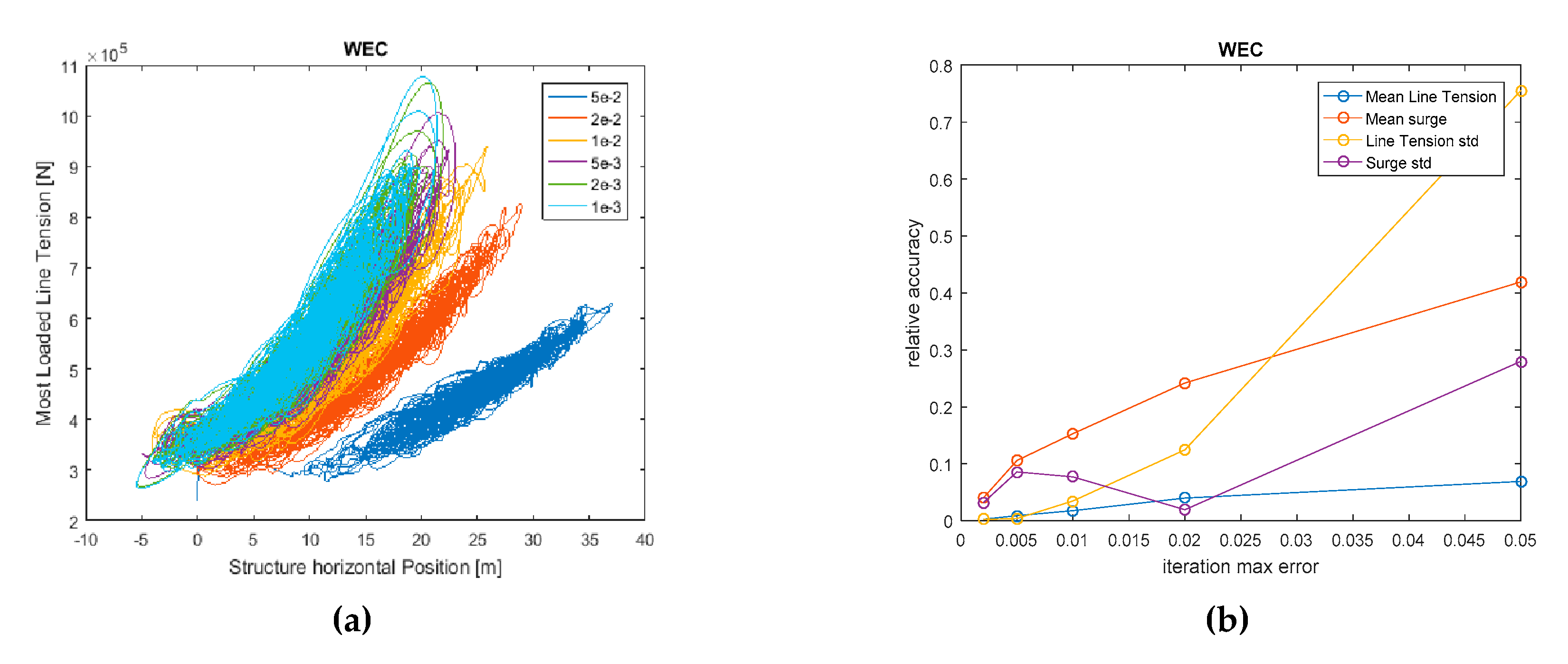
The QSTD model results are subject to the error allowed in the iterative process involved in the catenary equations. A sensitivity analysis has been carried out with the model presented in the previous section in order to check the accuracy of the mooring force with different relative errors allowed in the iterative loop.
It is shown in
Figure 2 that both line tension and structure horizontal position relative errors are found below 5% for a maximum allowed error in the catenary equations of 0.2%, assumed to be sufficiently accurate. This model has been proved to provide accurate results when using a time step of 0.1 s with a Newmark-beta integration scheme [
28].
2.5. Environmental Conditions
The simulation reference selected case corresponds to the combination of the recommended environmental conditions for permanent traditional offshore structures [
2], at the test site bimep [
29], and specified in
Table 1.
The environmental data has been taken from [
29], where an analysis of extreme climate conditions is presented for the site. The current velocity has been assumed constant over the depth of the floating WEC and the spectral shape used in the analysis has been JONSWAP with a peak shape parameter equal to 3.3. The corresponding load case assumes that waves, wind, and current are all aligned with one line of the mooring system. The wind force has not been considered for simplicity; therefore, the corresponding extreme value has been omitted in
Table 1.
2.6. Mooring Properties
The mooring system represented in the numerical model is a four-line catenary mooring system with the lines radially regularly distributed, as represented in
Figure 3. The fairleads of the mooring lines have been assumed to be located at the same height of the center of gravity of the FWEC to keep the stability in pitch of the buoy and avoid additional couplings between surge, heave, and pitch.
In order to find to what extent non-linearities of the mooring system influence the structure motions and line tensions, a range of realistic non-dimensional pretensions, as defined in Equation (6), and linear mass has been defined as specified in
Table 2, which results in 25 mooring models.
The vertical coordinate of the fairlead of the mooring lines with respect to the seabed has been assumed to be 150 m, assuming the fairleads at the center of gravity. Therefore, the resulting water depth is 181.97 m. It should be noted that the four mooring lines have been assumed to be of equal length for simplicity; however, detailed designs lines might result in different lengths if the probability of waves’ direction is accounted for. Therefore, the cost indicators to be introduced here must be seen as an upper bound provided for preliminary designs.
2.7. Numerical Model of the Floating Wave Energy Converter
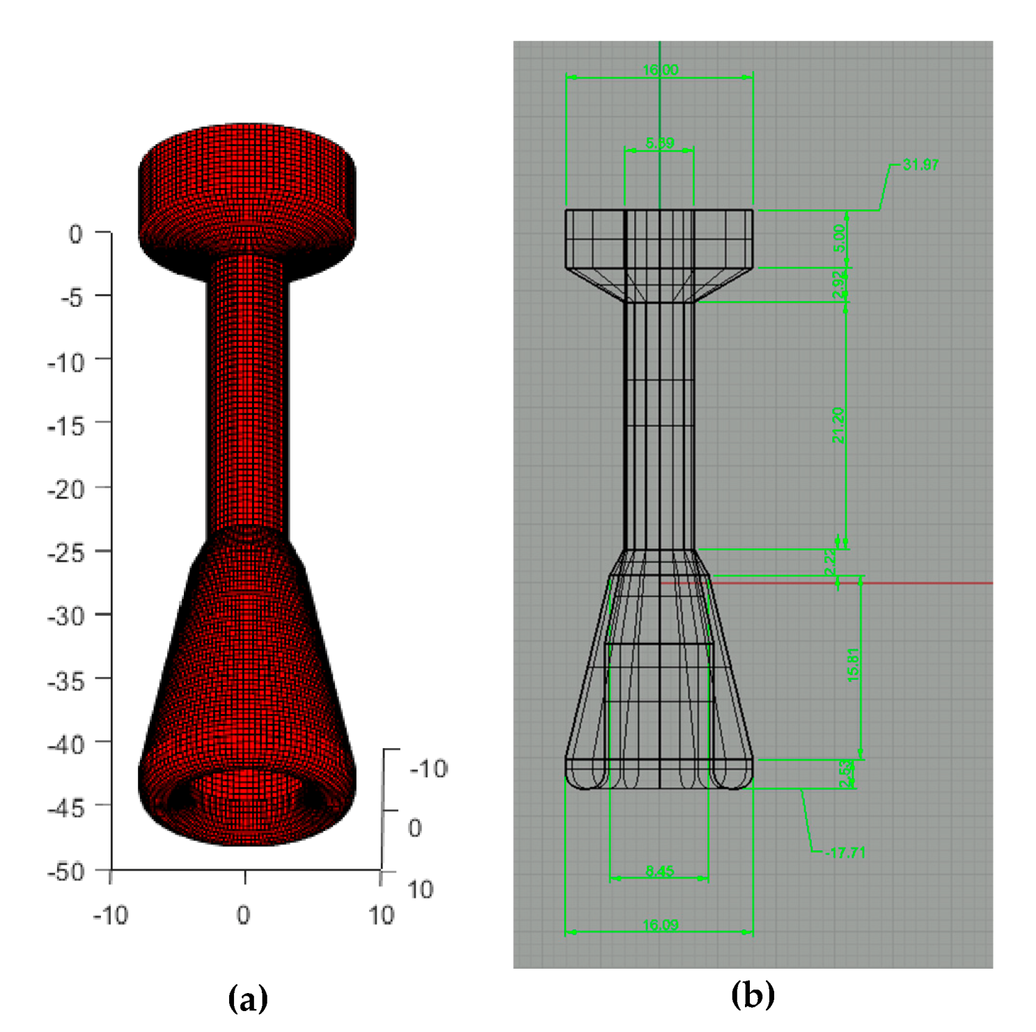
The FWEC geometry is based on the optimization presented in [
11], model ‘K’. It has also been modelled through linear potential theory and its mesh representation and main dimensions are shown in
Figure 4.
This geometry is designed to work as an OWC in which the power is extracted from the relative heaving motion of the represented structure in
Figure 4 with respect to the internal water column. The compressed and expanded air is made to pass through a self-rectifying air turbine allocated on the top deck of the floating structure. Its hydrodynamic properties for power production assessment can be modelled, among other methods, through two oscillating bodies. The coupled model consists of the one represented in
Figure 4 interacting with a massless surface representing the free surface water of the internal water column. In this paper, ULS is assessed, and it is assumed that the survival mode of operation can be approximated by the structure open at its top part. Therefore, the hydrodynamic model has been built up based on a single body, representing the structure.
The current steady force has been applied through a drag coefficient of 0.65 with an associated surface of 290 [m2]. Its total mass is 2.434 × 10⁶ [kg].
The quadratic damping force to account for the viscous damping has been considered adding the factors in
Table 3, computed assuming a common drag coefficient for cylinders of Cd = 0.8 [
31].
The non-linear drift force has been accounted for through the Newman approximation and based on the mean drift coefficients computed by the linear potential code.
3. Results
Results of the performance and cost indicators are introduced in this section. In order to compare the influence of the non-linear effects, the QSFD results have been considered as a baseline whilst the results of both DynTD and QSTD models are compared with the baseline.
3.1. Quasistatic Frequency Domain Model Results
In this approach, the horizontal stiffness computed at the mean position is added to the hydrostatic matrix to obtain the solution amplitudes. This method allows computing natural frequencies of the degrees of freedom of the structure. Since the mooring settings are variable, natural frequency in surge may vary between 0.03 rad/s and 0.07 rad/s. Natural frequencies of the structure in heave and pitch without mooring system have been found to be 0.67 rad/s and 0.38 rad/s, respectively.
Main performance factors to be considered when designing a mooring system are the maximum line tension and the maximum structure horizontal displacement. These parameters are relevant for the mooring system and umbilical cable structural integrity.
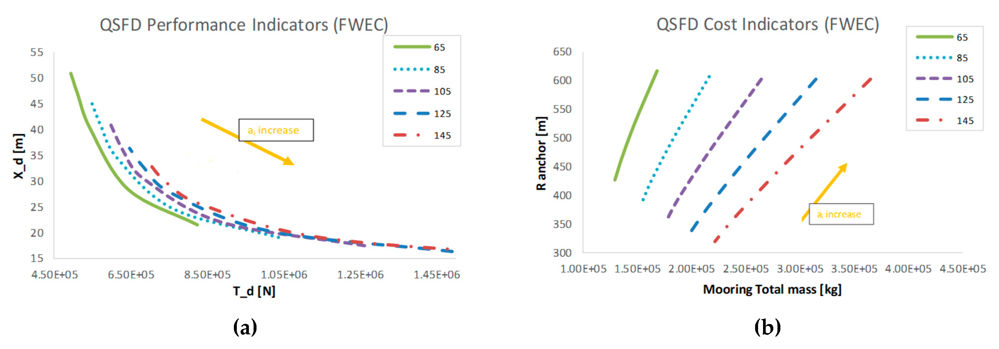
Each line in
Figure 5 represents a linear mass of the lines composing the mooring system and the variation of each performance and cost indicator along each linear mass is due to the variation in the non-dimensional pretension, within the values specified in
Table 2. A non-dimensional pretension (
) increase produces larger anchor radius (R_anchor) and lower design offset (X_d) in all cases.
A pretension increase influences the offset of the structure independently of the line mass; however, it also increases significantly the design tension, which may lead to unsafe designs as shown in
Figure 5 (left). The design offset of the structure is very sensitive to the linear mass at mid-low pretensions; however, with large pretensions, i.e.,
> 1.2, the variation of the offset due to the linear mass (65 kg/m–145 kg/m) becomes less significant.
Large pretensions imply in general larger footprints and total mooring mass, that are eventually translated into larger total costs of the mooring system. Similarly to what is observed for the offset, the anchor radius is very sensitive to the linear mass at mid-low pretensions; however, with high pretensions, the impact on the anchor radius is significantly lower, which is represented in
Figure 5 (right).
It should be pointed out that these baseline results indicate a requirement in the mooring total mass of 5–15% the mass of the structure, as long as lines are completely made up of a single chain type.
3.2. Performance Results of Non-Linear QSTD and DynTD Models
To quantify the uncertainty of the QSFD baseline indicators, results of both time domain models are introduced as factors with respect to the indicators introduced in
Figure 5. It enables quantifying the influence of non-linear effects such as the geometric stiffness or lines’ drag and inertia as well as coupling all degrees of freedom with the mooring system. In addition to the geometric stiffness and the mooring influence on all degrees of freedom, accounted for in the QSTD model, lines’ drag and inertia forces are also considered in the DynTD model.
Floater Dynamics
The most significantly excited degrees of freedom in the introduced numerical models are surge, heave, and pitch motions since all environmental forces have been aligned and propagated along the positive ‘x’ axis. These directly influence line tensions and the structural integrity of the umbilical cable that any WEC must have installed in order to transport electrical energy. These components are specially influenced by the surge motion of the structure, which corresponds to the horizontal offset in the case study here defined.
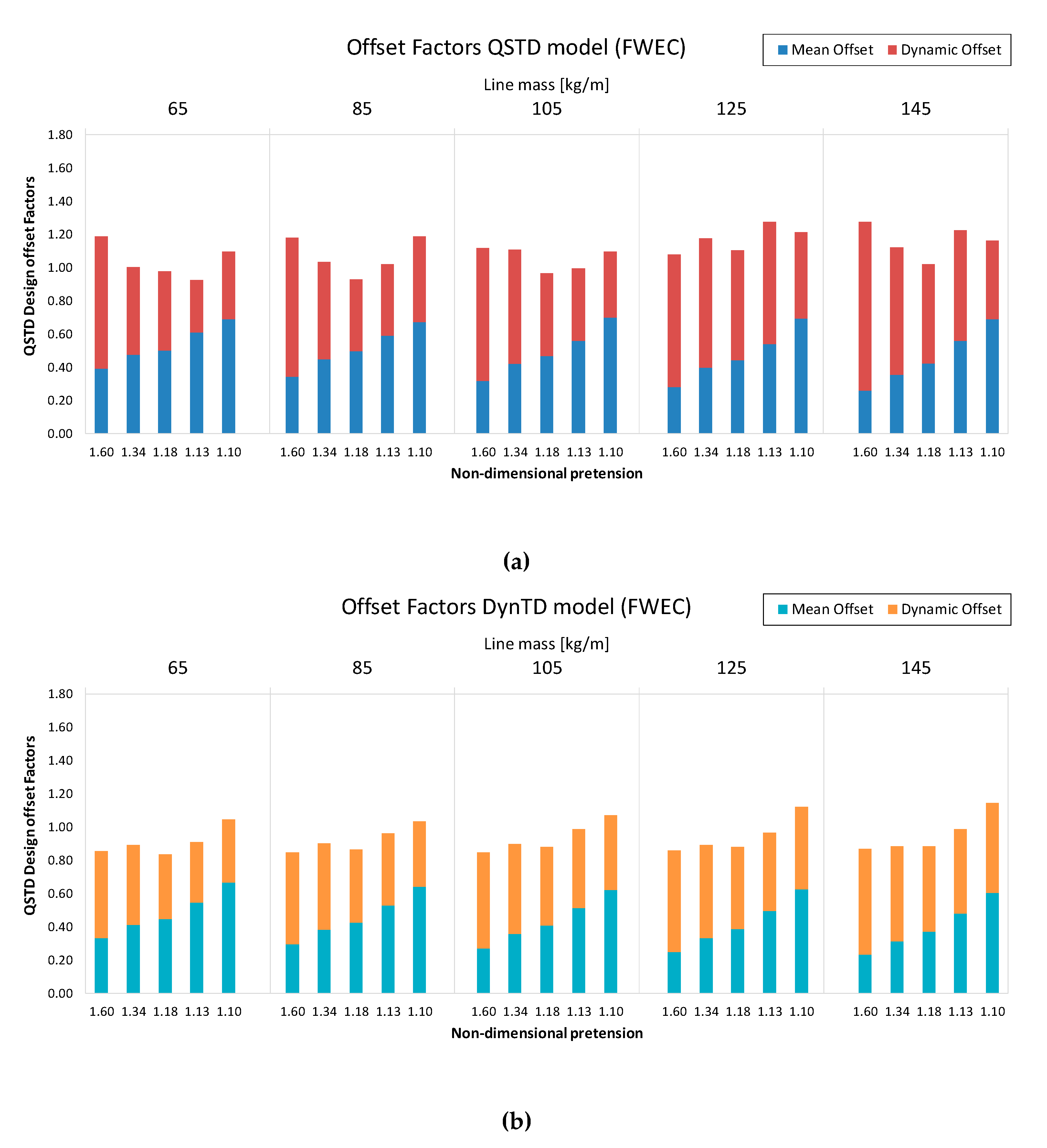
The FWEC shows in
Figure 6a balanced influence between the mean and dynamic surge on the design offset factors. Mean offset contribution is significantly increased as the non-dimensional pretension is decreased with slightly higher influence in the QSTD model. The total offset factor is dominated by structure dynamics with large non-dimensional pretensions and by the mean offset with low non-dimensional pretensions.
It is to be noted that most mooring models show factors <1 for the design offset with the DynTD model, whilst the QSTD model shows factors >1. It indicates, assuming that the most reliable model is the DynTD, that the QSFD model is more conservative in the estimation of the characteristic offsets of the structure rather than the QSTD for this kind of FWECs.
Design offset values shown in
Figure 6 have been estimated through the same procedure as carried out for lines tensions in each model, described in Equations (3) to (11).
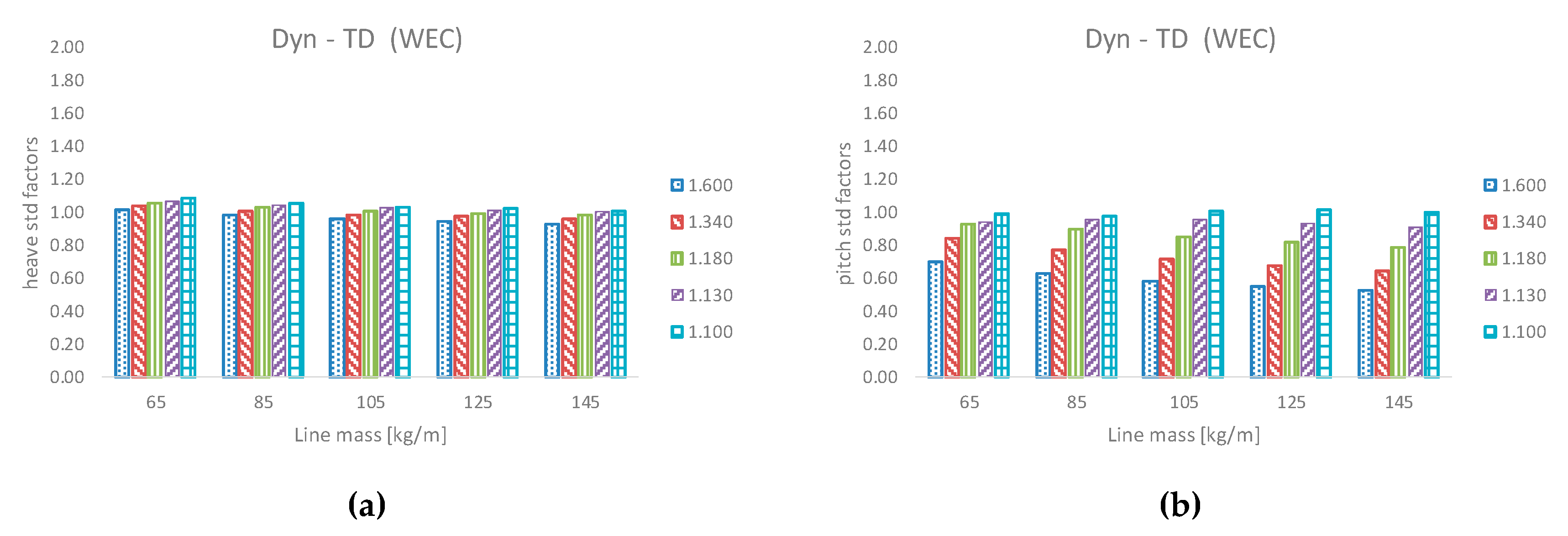
Factors of the QSTD approach in terms of heave and pitch std have been omitted as they show almost constant values, 15% to 20% in heave and −10% in pitch. Nevertheless, with the DynTD approach, heave factors have been observed within the range of −8% for high pretensions to 8% for low pretensions, as shown in
Figure 7 left. Pitch motion with the DynTD approach also shows increasing factors with a decreasing pretension, as observed in
Figure 7 right, though significantly more influenced by lines drag compared with heave.
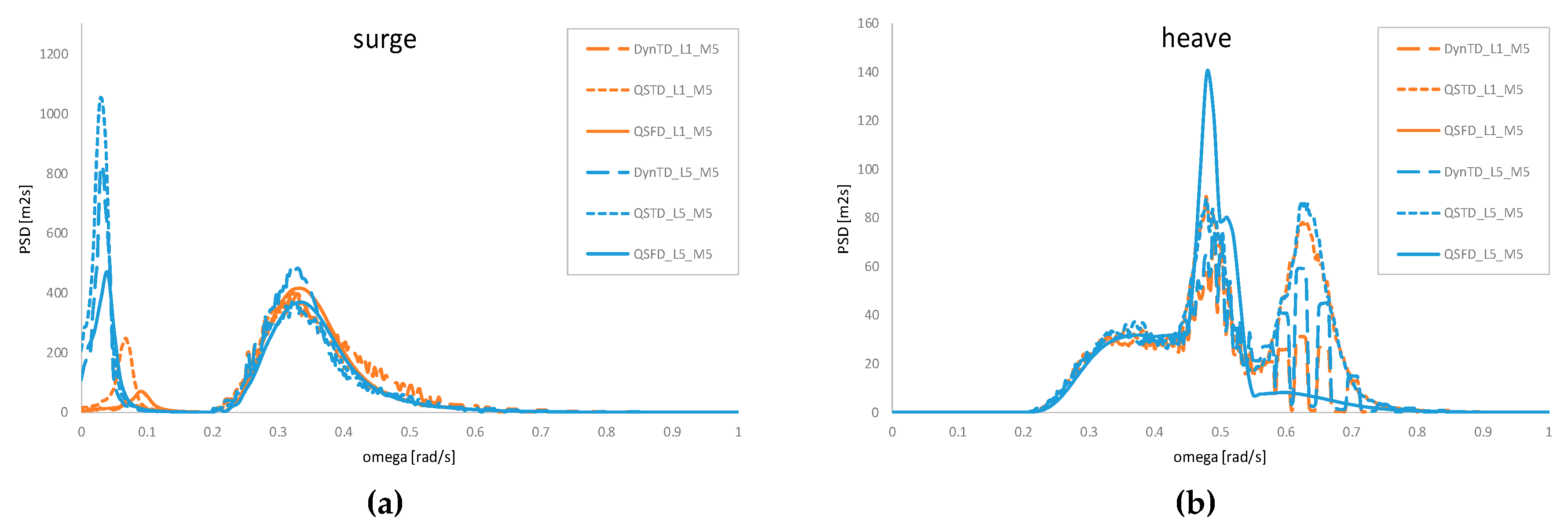
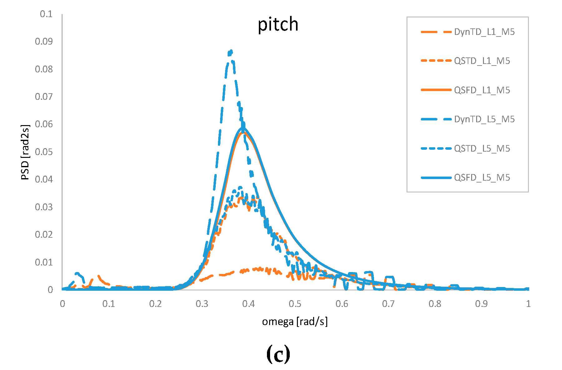
The increase of the std factor can be explained by looking at the PSDs of each degree of freedom, shown in
Figure 8. Surge motion is in general acceptably reproduced by the three models and there is good agreement in the natural frequency among all models, with PSDs showing very good agreement with low non-dimensional pretension. However, mooring systems with large non-dimensional pretensions show damped surge PSDs at the natural frequency with the DynTD models, which can be observed in
Figure 8 (left). Heave motion shows factors >1 in all cases as the heaving natural frequency is overdamped, which corresponds with the second peak in
Figure 8 (center), with the linearized QSFD model. Even though all time domain models show larger std in heave, DynTD models damp out slightly the heaving motion with respect to the QSTD, resulting in an underestimation of the QSFD and overestimation of the QSTD. Pitching motion std factors are due to the combination of two effects: on the one hand, the QSTD models do not catch entirely the surge-pitch coupling introduced by the mooring system, and on the other hand, large non-dimensional pretension models show damped surge PSDs in the DynTD models in the wave frequency range. Additionally, the QSFD model shows slightly underdamped PSDs in the wave frequency range, with respect to the TD models, which results in the −10% above-mentioned factors of the QSTD models. Therefore, mooring systems with large non-dimensional pretensions introduce significant damping in all degrees of freedom reducing the response, specially in the corresponding natural frequency.
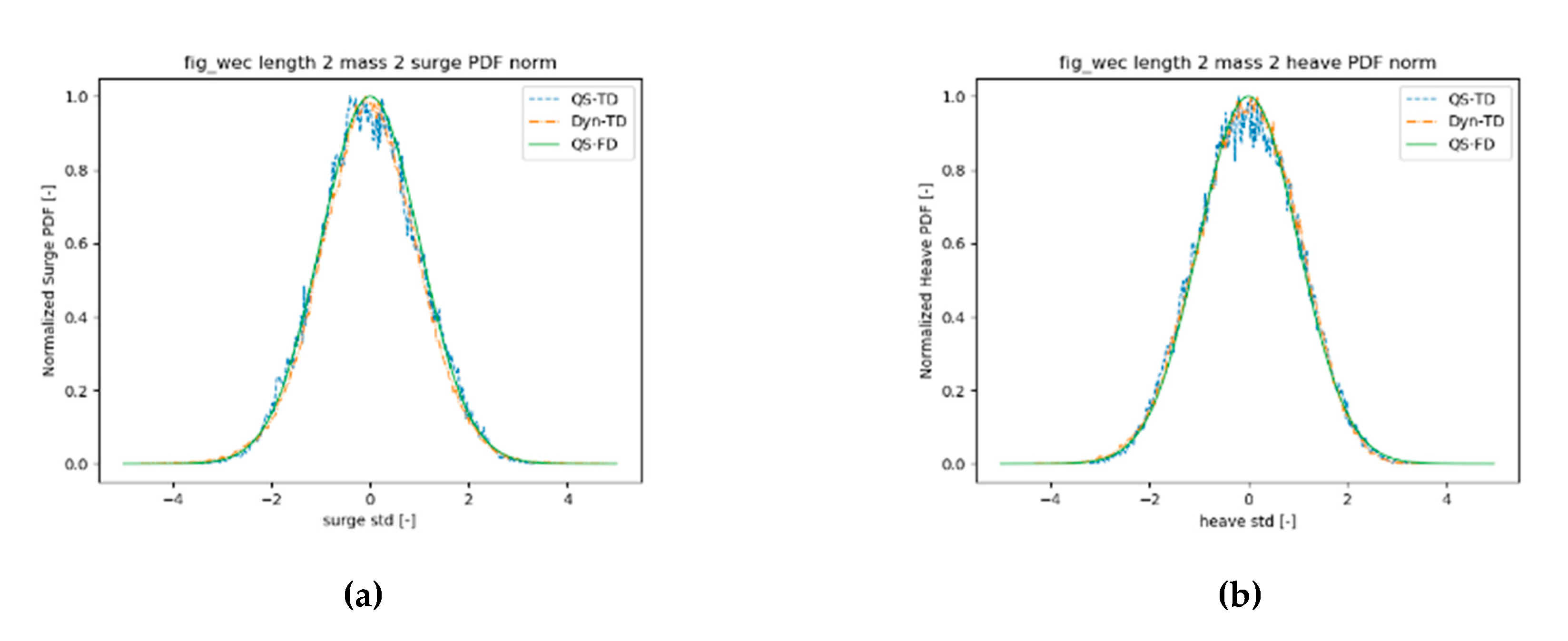
In
Figure 9 and
Table 4, probability distributions and their corresponding kurtosis (excess kurtosis with respect to the gaussian distribution) and skewness are introduced respectively for surge, heave, and pitch as well as for the most loaded line tension. The kurtosis indicates the higher or lower probability of producing extreme values, respectively, depending if its value is higher or lower than 3, the kurtosis of the Gaussian distribution. In
Table 4, the corresponding values of the QSFD models have been omitted since it is a linear model and, therefore, they are Gaussian distributed with kurtosis equal to 3. The skewness indicates the asymmetry of the distribution, Gaussian distributions have zero skewness, and it is also not included.
All degrees of freedom show negative excess kurtosis and skewness with the QSTD models, with very homogeneous values among the models here assessed, whose mean values are shown in
Table 4. Nevertheless, the most loaded line tension shows positive excess kurtosis as well as skewness. It is coherent with the catenary equations as it restricts floater motions through a non-linear increase of line tensions with the offset increase. It therefore leads to lower extreme motion and higher extreme tension values with respect to the linearized QSFD. The most influenced degree of freedom is the pitch motion along with the most loaded line tension, whilst heave and surge do not differ significantly from the equivalent linear PDF, as represented in
Figure 9.
Including lines’ drag and inertia, structure motions are modified as already pointed out in the PSD analysis. The heaving motion also shows homogeneous excess kurtosis and skewness among the mooring models with the DynTD approach and its values are shown in
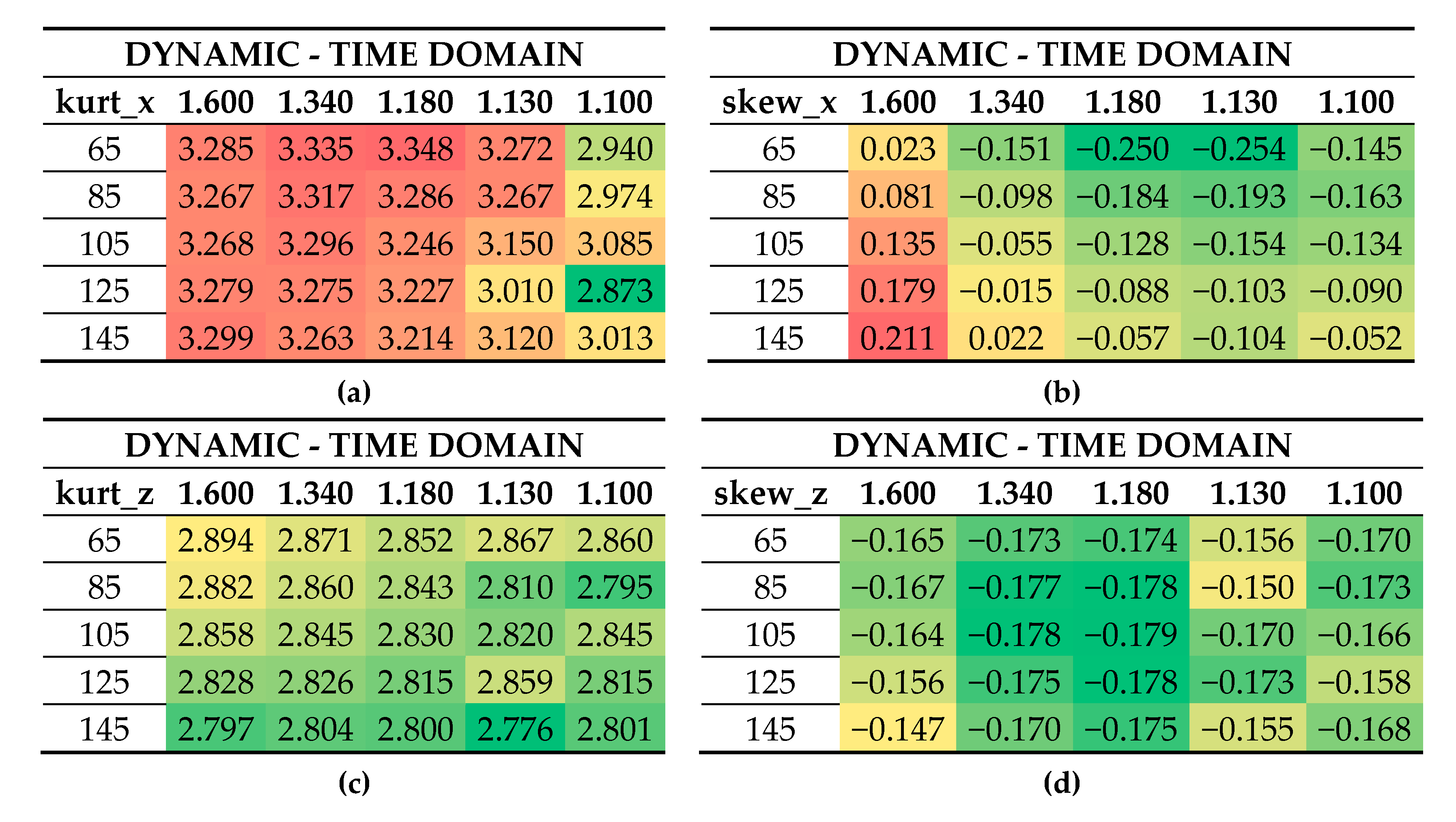
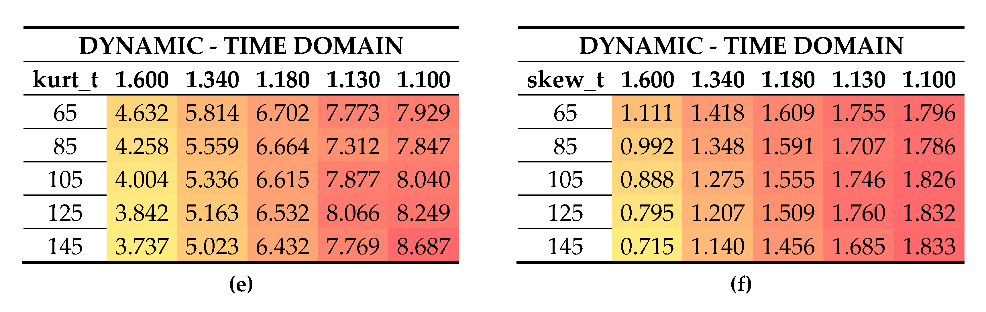
Figure 10. Surge, pitch, and most loaded line tensions show variable values depending mostly on the non-dimensional pretension. Surge motion shows higher positive kurtosis with higher pretensions and a kurtosis closer to 3 as the pretension is decreased. The skewness tends towards negative values with lower pretensions and shows a tendency to the values represented with the QSTD approach. It indicates that the fact that the natural frequency is damped out in the PSD of DynTD models; this is due to performing very non-linear motions with high pretensions, making it more difficult to obtain good estimations of extreme surge motions with QSFD models. Pitching motion shows the same tendency as showed by surge and its results have been omitted here for simplicity.
4. Predicted Line Tensions
The design line tension has been computed for all cases as defined in Equations (5), (10) and (11). The differences come from the non-linearities included in each model i.e., the non-linear geometric stiffness and line’s drag and inertia forces.
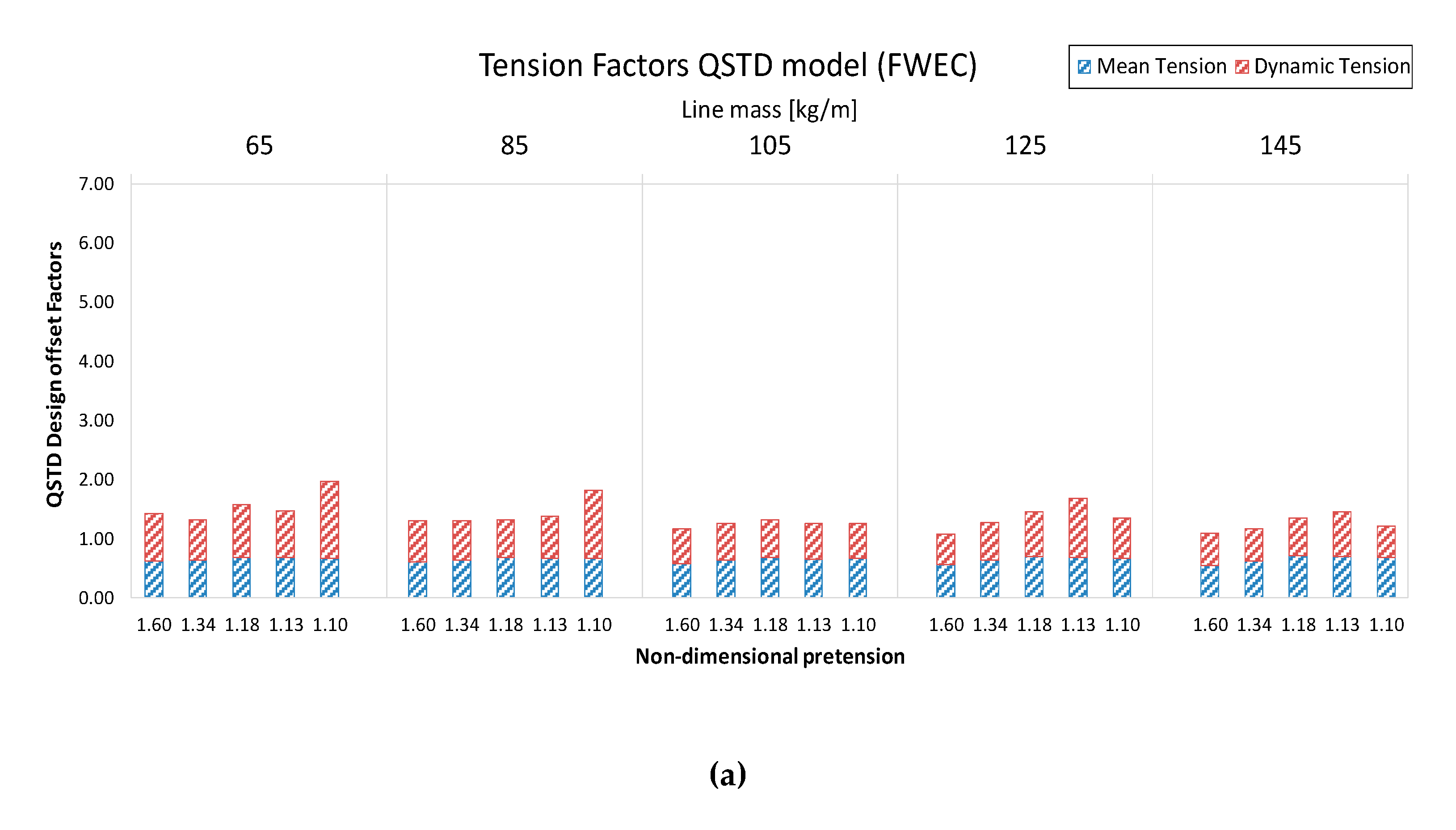
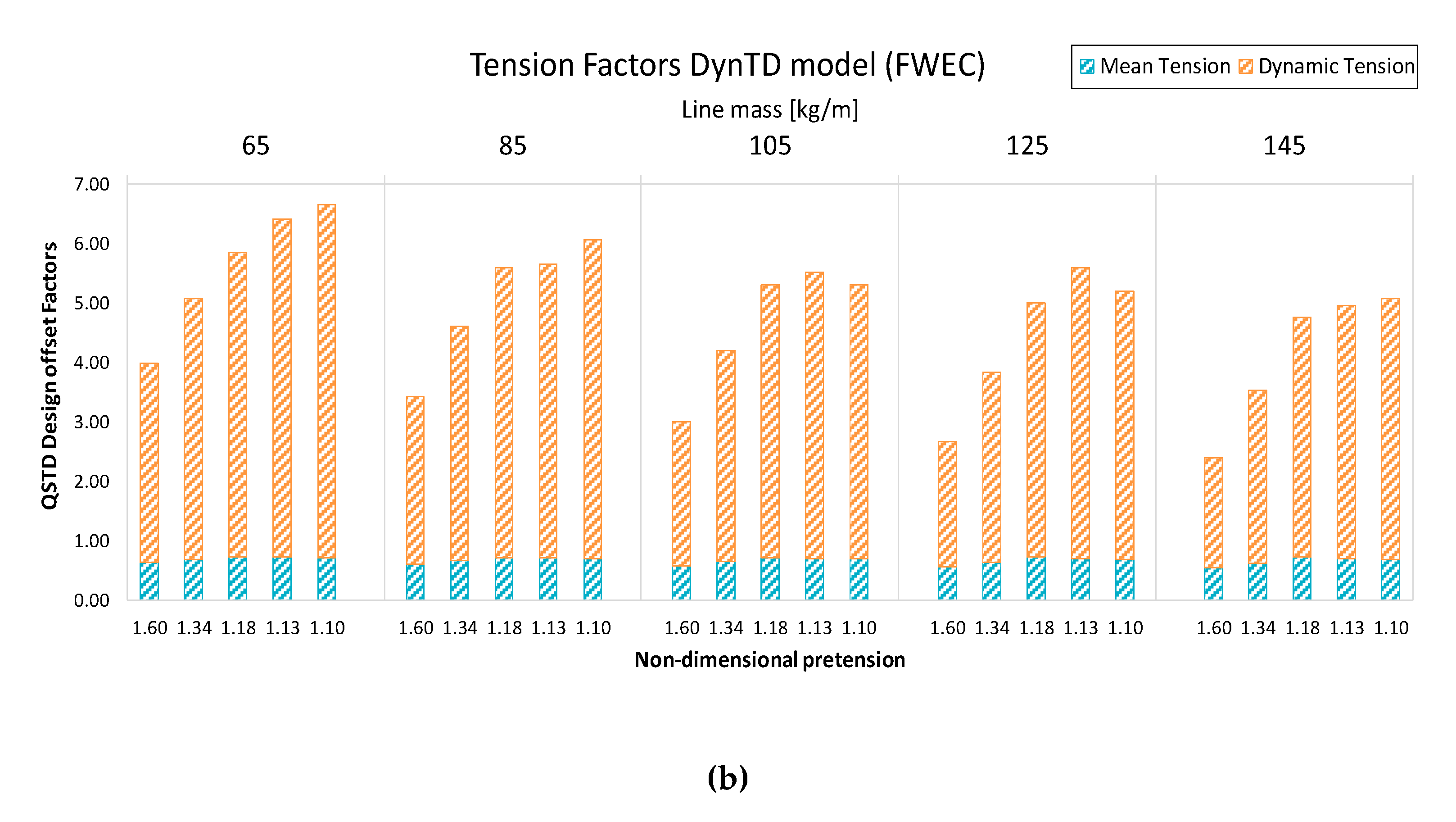
The mean line tension shows contributions of 55%–75% on the design line tension and is not significantly sensitive to the mooring settings; the observed differences are driven by line tensions induced by structure dynamics. The QSTD approach shows factors of 1.5 to 2 with a partially increasing tendency with decreasing pretensions in
Figure 11. Nevertheless, in contrast to the tendency of structure motions to perform more linear motions with low non-dimensional pretensions, lines’ tensions with the DynTD approach show larger discrepancies of the design tension factors as the pretension is increased, of up to 6 with low pretensions, which can be observed in
Figure 11. The QSTD approach shows a clear positive skewness and excess kurtosis in accordance with the shape of the catenary curves, as represented in [
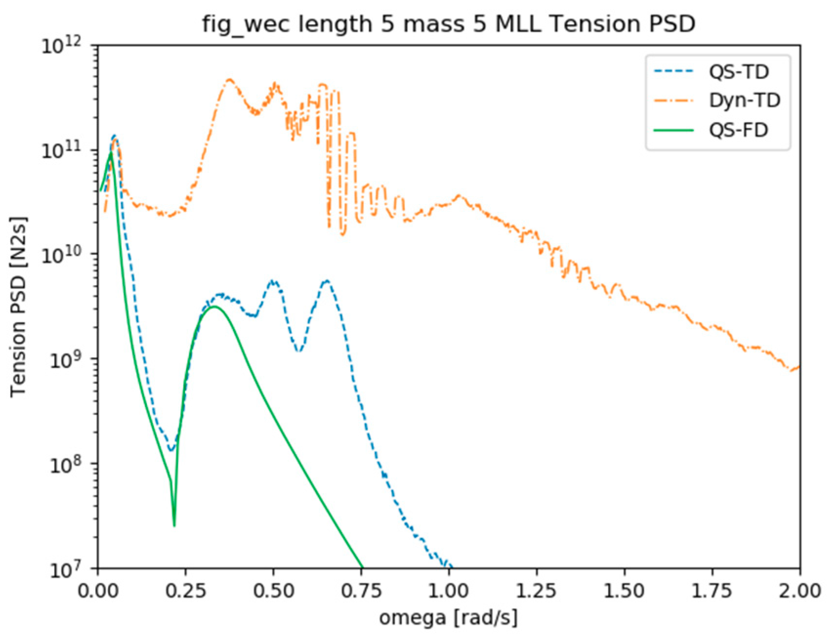
21]. It is a consequence of both the non-linear stiffness and the coupling with heave, as observed in the PSD of the line tension in
Figure 12.
The most loaded line tensions with the DynTD approach show PDFs with two local maxima as represented in
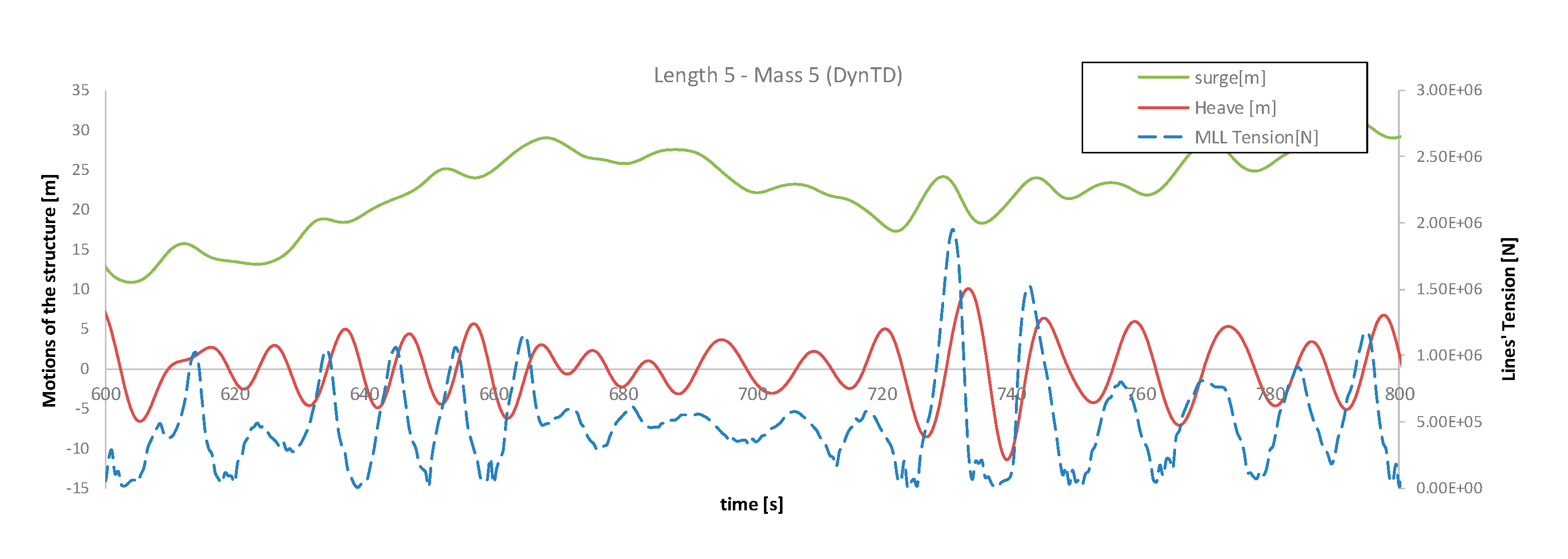
Figure 13. The maximum at higher tensions is due to surge dynamics, which tends to perform more similarly to the QSTD model. However, the peak at lower tensions is due to slack lines during certain instants, which occurs due to the heaving of the buoy and to lines’ inertia. It is clearly observed in
Figure 14, where a clear correlation of slack line instants with negative heave velocity is observed and not showing a clear correspondence with surge dynamics. In
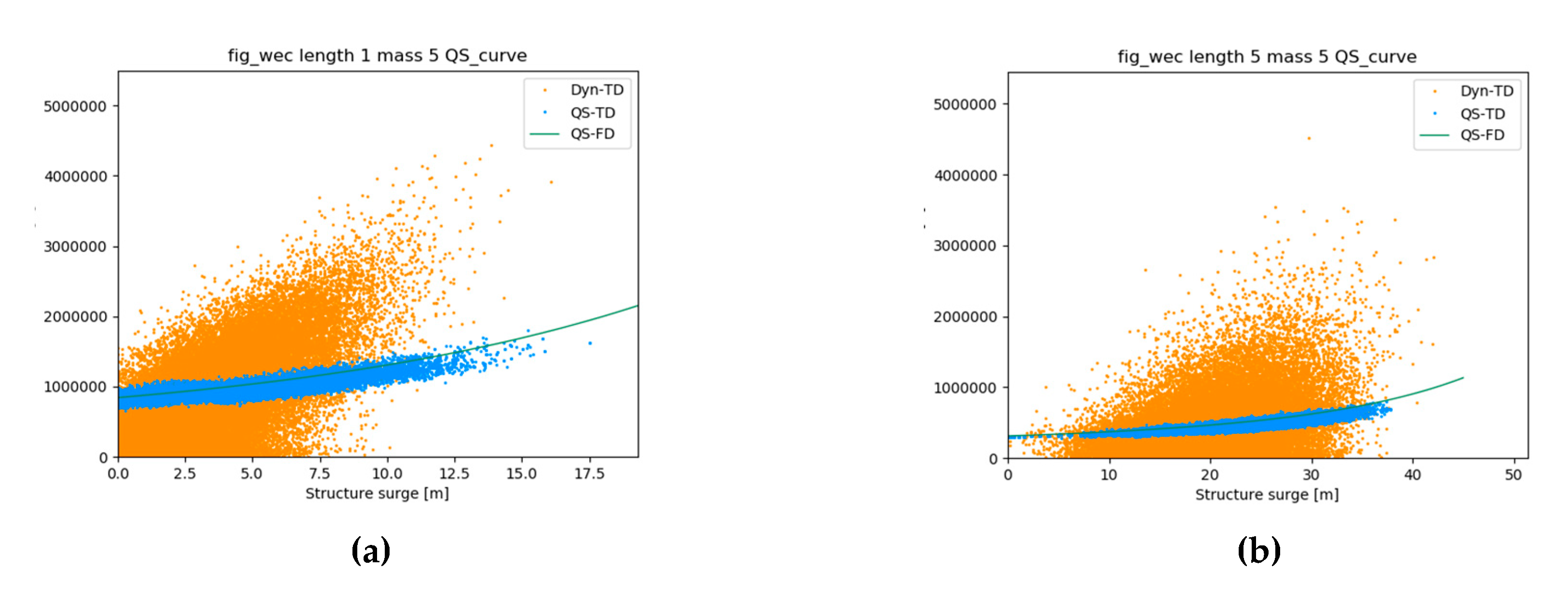
Figure 15, the QSTD approach shows a significant variability in line tension with respect to the quasistatic curve as a consequence of the structure’s heaving; however, the DynTD approach shows a very large line tension dispersion due to the lines’ inertia, an effect that cannot be reproduced with either the QSFD or the QSTD models, leading to significantly underestimating lines tension. On the other hand, looking at the low frequency range in
Figure 12, there is good agreement between the QSTD and DynTD as it appears to be decoupled from the heaving motion.
Consequently, even though the estimation of lines’ tension with the QSTD approach shows the influence of the heaving motion with respect to the QSFD, both of them differ significantly with respect to the DynTD with high pretensions mainly due to the lines’ induced damping and with low pretensions due to the lines’ inertia.
5. Discussion
The QSFD approach shows decreasing design offsets of the structure and increasing design tensions when increasing the pretension, with any linear mass. However, it also implies increasing required footprints and total mass. Even though moderate pretensions have been observed as a mechanism to limit the offset, it has also been showed in
Figure 5 that with high pretensions, i.e., >1.2, there is no additional benefit obtained, in terms of offset or footprint, whilst the mooring system is exposed to higher line tensions.
Results of the QSTD and DynTD approaches have been compared with the QSFD baseline results. The design offset, related with the surge motion, shows higher values with the QSTD approach than with the QSFD approach, mainly due to the response in the low frequency range. Its design offsets have been observed in
Figure 6 to be driven by the dynamic motions with high pretensions and by the mean offset with low pretensions. Similar tendencies are found with the DynTD approach; however, due to the viscous drag of the lines, the surge natural frequency is significantly damped out with high pretensions and design offsets show increasing factors with decreasing pretensions, showing values, in general, lower than with the QSFD. It means that the QSFD estimates, even though the natural frequency is slightly shifted, are more consistent with the DynTD approach than those of the QSTD, mainly as a consequence of the overdamping introduced by the linearization in the frequency domain, which partially covers lines’ viscous drag, accounted for in the DynTD approach. Nevertheless, the QSTD approach reproduces more accurately the low frequency response of the floater and, hence, the corresponding line tension.
Heave motions show larger std values with the QSTD than with the QSFD; the latter uses a linearized viscous drag, which overdamps the heaving natural frequency of the structure. The DynTD approach shows increasing heaving factors with respect to the QSFD approach. Even though heaving PSDs in the natural frequency of the structure are overdamped with the QSFD approach, the peak at a lower frequency (around 0.5 rad/s) shows higher responses, related with resonance of the internal water column. It shows factors of heave std values in
Figure 7 increasing from −8% to 8% as the non-dimensional pretension is increased. Pitch motions show the same trend as heaving motions; however, the linearized viscous drag with the QSFD shows an underdamped PSD compared to that of the QSTD and, therefore, QSTD factors are <1. Adding viscous drag forces on lines in the DynTD approach implies, as pointed out for surge and heave, std values close to the QSFD results with decreasing non-dimensional pretension.
In order to assess the degree of linearity of the responses, probability density functions have also been analyzed. As observed in the standard deviations, QSTD approach shows very regular excess kurtosis and skewness among all mooring models, with negative kurtosis and skewness in all degrees of freedom and positive for the most loaded line tension. It is coherent with the catenary equations where small motions imply a non-linear increase of lines tensions, commonly fitted with third order polynomials for practical applications. Heave motion with the DynTD model shows also balanced values among all mooring models, which, together with what is observed in the std values, points at no significant influence of lines’ viscous drag and inertia on the heaving motion. On the other hand, both surge and pitch motions are significantly influenced by lines’ drag and inertia, resulting in increasingly non-linear PDFs as the non-dimensional pretension is increased. With the DynTD approach all motions show in
Figure 10, a tendency to be more linear and closer to the QSFD results in mid to low non-dimensional pretensions, i.e., <1.2.
Looking at the results of the most loaded line tension, factors of the QSTD with respect to the QSFD are not excessively sensitive to the mooring settings, showing std factors of 1.5 to 2 in
Figure 11 (left). It has been found to be mainly due to the influence of the heaving motion on lines PSDs as well as the positive excess kurtosis and skewness, introduced by the geometric stiffness. However, the DynTD approach shows, unlike to what is observed in the structure’s motions, increasing factors with decreasing non-dimensional pretension, showing values from 3 up to 7 in
Figure 11 (right). Even though the higher damping introduced by the viscous drag force on lines with high pretensions is translated into higher line tensions, mooring models with lower pretensions are increasingly influenced by lines inertia. It is explained looking at the time series showed in
Figure 14, where heaving motions moving downwards and upwards with high velocities produce slack lines and the subsequent snap load, respectively. It results in high probabilities of close to zero line tensions as well as of relatively high line tensions. This effect is a consequence of lines inertia, more significative as the pretension is lowered, and can only be reproduced with the DynTD approach.
Mooring cost optimization is most accurate with the DynTD approach, even though the QSTD would provide acceptably good cost indicators, due to the required simulation time of the QSTD and in lieu of any additional accuracy in terms of line tensions, comparison of cost optimisations has been carried out between the QSFD and the DynTD approaches (
Figure 18). Both approaches have shown higher total cost and lower optimum linear mass with increasing mooring pretension. Nevertheless, the estimates of the required mass and area with high pretensions are underestimated by the QSFD approach and it has been found to be applicable with mid to low non-dimensional pretensions (i.e., <1.2) to set design tendencies in early stages. The QSFD approach provides a generally underestimated total cost and optimum linear mass that after correction with the functions provided in
Figure 17 becomes reasonably usable for early mooring design stages.
6. Conclusions
In the present work, a comparison between three different numerical models of a floating wave energy converter moored by means of a four-line catenary mooring system has been analysed with 25 mooring setting combinations. A linearized frequency domain model (QSFD), a non-linear quasistatic time domain model (QSTD), and a non-linear dynamic model (DynTD) are the three approaches here compared.
A spar type floating wave energy converter (FWEC) has been modelled as a case study. The FWEC has been assumed to be an oscillating water column, working in survivability mode.
The environmental conditions have been assumed to reproduce extreme conditions in the bimep test site. Simulations have been carried out for 25 combinations arising from 5 linear mass and 5 lines non-dimensional pretensions of the mooring system. The selected lines pretension and linear mass have been selected so that realistic buoy offsets are obtained.
It has been found that the influence of viscous drag force on lines is most significant with high non-dimensional pretensions, damping out the natural frequency in all degrees of freedom. It influences most surge and pitch motions; however, its PSDs tend to show more linear motions as the non-dimensional pretension is decreased. The same can be stated for the heaving motion; however, its influence is not significant and the linearized drag force in the QSFD tends to slightly underestimate heaving PSDs. Therefore, buoy motions can be acceptably estimated with the three approaches with low non-dimensional pretensions, while only DynTD is recommended for high pretensions, i.e., >1.2.
Most loaded line tensions show the influence of the heaving motion with the QSTD model and results in slightly higher PSDs than with the QSFD. The QSTD also shows the non-linearity introduced by the geometric stiffness on lines’ PDFs increasing the design tension. Nevertheless, heave motions in the DynTD approach induces slack lines and the subsequent snap load cycles and the design line tensions are increased to almost an order of magnitude with respect to the other two approaches. Consequently, as the non-dimensional pretension is decreased, snap loads are more occurrent and line tensions become more non-linear, showing increasingly higher design tensions. Consequently, the most appropriate approach to estimate line tensions is the DynTD approach for line tension estimates in extreme environmental states; however, in cases where only low frequency motions are of interest, the QSTD approach is very consistent with the DynTD for line tension assessment.
Total mooring cost indicators optimizations generally result in higher total costs with higher non-dimensional pretensions and higher optimum linear mass with lower non-dimensional pretensions. Even though the QSTD approach shows more accurate total cost compared with the QSFD, it is not worth being used for early optimizations due to its required computational time, as it does not provide sufficient accuracy of lines’ performance. Found differences in terms of cost and line tension have been found to be mostly functions of non-linear pretensions and linear functions have been proposed so that the QSFD cost and tension results can be acceptably corrected. Therefore, QSFD has proved to show, after applying the corresponding correction factors, acceptable optimization tendencies for non-dimensional pretensions < 1.2, while high pretensions require the DynTD approach.
In order to account for operational sea states during preliminary design stages, models that account for lines inertia and drag would be very convenient. Nevertheless, the large number of environmental states and the required simulation lengths and time sometimes may dissuade designers from doing it for a significant number of mooring configurations. Because of its lower computational burden, the frequency domain approach, despite its limitation to capture nonlinear effects, can be corrected with the proposed factors to cover the nonlinear effects and, hence, can be used at early design stages and during concept selection. The authors are currently working on a lumped mass mooring and solid rigid body motions coupled model which, after linearization, can be solved in the frequency domain, accounting for line dynamics to be used under low to moderate environmental states, in which the mooring can be acceptably linearized, keeping the computational cost under the same levels of the QSFD here introduced.
Author Contributions
Conceptualization, I.T. and B.d.M.; methodology, I.T. and B.d.M.; software, I.T.; validation, I.T. and V.N.; formal analysis, I.T.; investigation, I.T., V.N., and V.P.; resources, I.T., V.N., and V.P.; data curation, I.T.; writing—original draft preparation, I.T.; writing—review and editing, I.T., V.N., B.d.M., and V.P.; visualization, I.T., V.N., B.d.M., and V.P.; supervision, V.N. and V.P.; project administration, V.P.; funding acquisition, V.N. and V.P. All authors have read and agreed to the published version of the manuscript.
Funding
This research was funded by Project IT949-16 given by the Departamento de Educación, Política Lingüística y Cultura of the Regional Government of the Basque Country; by the Basque Business Development Agency ELKARTEK 2019 programme, under grant KK-2019/00085, MATHEO project; and by the Regional Government of the Basque Country and European Union through European Funds for Regional Development, HAZITEK 2019 program, under grant ZE-2019/00886, WECAM project.
Conflicts of Interest
The authors declare no conflict of interest.
References
- OES. News. International LCOE for Ocean Energy Technology. Available online: https://www.ocean-energy-systems.org/news/international-lcoe-for-ocean-energy-technology/ (accessed on 16 March 2020).
- Offshore Standards. DNVGL-OS-E301: Position Mooring. Edition July 2018. Available online: http://rules.dnvgl.com/docs/pdf/dnvgl/os/2018-07/dnvgl-os-e301.pdf (accessed on 16 March 2020).
- NI 461 DTO R00 E—Quasi-Dynamic Analysis of Mooring Systems Using Ariane Software. Available online: https://link.springer.com/chapter/10.1007/978-981-15-0291-0_152 (accessed on 16 March 2020).
- Azcona, J.; Munduate, X.; González, L.; Nygaard, T.A. Experimental validation of a dynamic mooring lines code with tension and motion measurements of a submerged chain. Ocean Eng. 2017, 129, 415–427. [Google Scholar] [CrossRef]
- Hall, M.; Goupee, A. Validation of a lumped-mass mooring line model with DeepCwind semisubmersible model test data. Ocean Eng. 2015, 104, 590–603. [Google Scholar] [CrossRef]
- Touzon, I.; Nava, V.; Gao, Z.; Mendikoa, I.; Petuya, V. Small scale experimental validation of a numerical model of the HarshLab2.0 floating platform coupled with a non-linear lumped mass catenary mooring system. Ocean Eng. 2020, 200, 107036. [Google Scholar] [CrossRef]
- Vu, M.T.; Choi, H.-S.; Kang, J.; Ji, D.-H.; Jeong, S.-K. A study on hovering motion of the underwater vehicle with umbilical cable. Ocean Eng. 2017, 135, 137–157. [Google Scholar] [CrossRef]
- Vu, M.T.; Van, M.; Bui, D.H.P.; Do, Q.T.; Huynh, T.T.; Lee, S.D.; Choi, H.S. Study on Dynamic Behavior of Unmanned Surface Vehicle-Linked Unmanned Underwater Vehicle System for Underwater Exploration. Sensors 2020, 20, 1329. [Google Scholar] [CrossRef]
- Amaechi, C.V.; Wang, F.; Hou, X.; Ye, J. Strength of submarine hoses in Chinese-lantern configuration from hydrodynamic loads on CALM buoy. Ocean Eng. 2019, 171, 429–442. [Google Scholar] [CrossRef]
- Antonio, F.d.O. Wave energy utilization: A review of the technologies. Renew. Sustain. Energy Rev. 2010, 14, 899–918. [Google Scholar] [CrossRef]
- Gomes, R.P.F.; Henriques, J.C.C.; Gato, L.M.C.; Falcão, A.F.O. Hydrodynamic optimization of an axisymmetric floating oscillating water column for wave energy conversion. Renew. Energy 2012, 44, 328–339. [Google Scholar] [CrossRef]
- Doyle, S.; Aggidis, G.A. Development of multi-oscillating water columns as wave energy converters. Renew. Sustain. Energy Rev. 2019, 107, 75–86. [Google Scholar] [CrossRef]
- da Fonseca, F.C.; Gomes, R.P.F.; Henriques, J.C.C.; Gato, L.M.C.; Falcão, A.F.O. Model testing of an oscillating water column spar-buoy wave energy converter isolated and in array: Motions and mooring forces. Energy 2016, 112, 1207–1218. [Google Scholar] [CrossRef]
- Falcão, A.F.O.; Sarmento, A.J.; Gato, L.M.C.; Brito-Melo, A. The Pico OWC wave power plant: Its lifetime from conception to closure 1986–2018. Appl. Ocean Res. 2020, 98, 102104. [Google Scholar] [CrossRef]
- Marine Energies—EVE. Available online: https://eve.eus/Actuaciones/Marina?lang=en-gb (accessed on 6 June 2020).
- MARMOK-A-5 Wave Energy Converter. Tethys. Available online: https://tethys.pnnl.gov/project-sites/marmok-5-wave-energy-converter (accessed on 6 April 2020).
- Nielsen, K.; Wendt, F.; Yu, Y.H.; Ruehl, K.; Touzon, I.; Nam, B.W.; Kim, J.S.; Kim, K.-H.; Crowley, S.; Sheng, W. OES Task 10 WEC heaving sphere performance modelling verification. Presented at the 3rd International Conference on Renewable Energies Offshore (RENEW 2018), Lisbon, Portugal, 8–10 October 2018. [Google Scholar]
- Wendt, F.; Nielsen, K.; Yu, Y.H.; Bingham, H.; Eskilsson, C.; Kramer, M.; Babarit, A.; Bunnik, T.; Costello, R.; Crowley, S. Ocean Energy Systems Wave Energy Modelling Task: Modelling, Verification and Validation of Wave Energy Converters. J. Mar. Sci. Eng. 2019, 7, 379. [Google Scholar] [CrossRef]
- Penalba, M.; Mérigaud, A.; Gilloteaux, J.-C.; Ringwood, J.V. Influence of nonlinear Froude–Krylov forces on the performance of two wave energy points absorbers. J. Ocean Eng. Mar. Energy 2017, 3, 209–220. [Google Scholar] [CrossRef]
- Pinkster, J.A. Mean and low frequency wave drifting forces on floating structures. Ocean Eng. 1979, 6, 593–615. [Google Scholar] [CrossRef]
- Touzon, I.; de Miguel, B.; Nava, V.; Petuya, V.; Mendikoa, I.; Boscolo, F. Mooring System Design Approach: A Case Study for MARMOK-A Floating OWC Wave Energy Converter. Presented at the ASME 37th International Conference on Ocean, Offshore and Arctic Engineering, Madrid, Spain, 17–22 June 2018. [Google Scholar] [CrossRef]
- Fitzgerald, J.; Bergdahl, L. Including moorings in the assessment of a generic offshore wave energy converter: A frequency domain approach. Mar. Struct. 2008, 21, 23–46. [Google Scholar] [CrossRef]
- Larsen, K.; Sandvik, P.C. Efficient Methods for the Calculation of Dynamic Mooring Line Tension. Presented at the First ISOPE European Offshore Mechanics Symposium, Seoul, Korea, 24–28 June 1990. [Google Scholar]
- Low, Y.M.; Langley, R.S. Time and frequency domain coupled analysis of deepwater floating production systems. Appl. Ocean Res. 2006, 28, 371–385. [Google Scholar] [CrossRef]
- Cummins, W.E. The Impulse Response Function and Ship Motions. Presented at the Symposium of Ship Theory, Hamburg, Germany, 25–27 January 1962; Institut für Schiffbau der Universität Hamburg: Hamburg, Germany, 1962. [Google Scholar]
- van den Boom, H.J.J. Dynamic Behaviour of Mooring Lines. In Proceedings of the Behaviour of Offshore Structures, Delft, The Netherlands, 1–5 July 1985; Elsevier Science Publishers B.V.: Amsterdam, The Netherlands, 1985. [Google Scholar]
- OrcaFlex. Dynamic Analysis Software for Offshore Marine Systems. Available online: https://www.orcina.com/orcaflex/ (accessed on 15 December 2019).
- Naess, A.; Moan, T. Stochastic Dynamics of Marine Structures; Cambridge University Press: Cambridge, UK, 2012. [Google Scholar]
- Metocean Analysis of BiMEP for Offshore Design TRLplus. IH-Cantabria, bimep, 2017. Available online: https://trlplus.com/wp-content/uploads/2017/03/Metocean_Analysis_of_BiMEP_for_Offshore_Design_TRLplus_March_2017.pdf (accessed on 19 March 2020).
- MATLAB. El Lenguaje del Cálculo Técnico. MATLAB & Simulink. Available online: https://es.mathworks.com/products/matlab.html (accessed on 5 July 2020).
- DNV-RP-C205. Environmental Conditions and Environmental Loads; Det Norske Veritas: Oslo, Norway, 2010. [Google Scholar]
Figure 1.
Non-dimensional pretension line shapes for axial stiffness EA = 1e9 [N].
Figure 1.
Non-dimensional pretension line shapes for axial stiffness EA = 1e9 [N].
Figure 2.
Sensitivity analysis of the QSTD model to the iterative process of the catenary equations. Surge of the structure and the corresponding mooring horizontal force (a) and relative errors of the standard deviation with different relative errors allowed in the catenary equations of both line tension and surge motion (b).
Figure 3.
Four lines mooring system configuration modeled for both structures in 150 m water depth. Visualization of the QSTD model developed on Matlab [
30] (
a) and the DynTD model on Orcaflex [
27] (
b).
Figure 3.
Four lines mooring system configuration modeled for both structures in 150 m water depth. Visualization of the QSTD model developed on Matlab [
30] (
a) and the DynTD model on Orcaflex [
27] (
b).
Figure 4.
Mesh representation of the boundary element method (BEM) model for the FWEC spar platform submerged part (
a) and its main dimensions [m] with the reference at its CoG (
b). Reproduced from [
11] (Renewable Energy 44 (2012) 328–339), corresponding to model ‘K’.
Figure 4.
Mesh representation of the boundary element method (BEM) model for the FWEC spar platform submerged part (
a) and its main dimensions [m] with the reference at its CoG (
b). Reproduced from [
11] (Renewable Energy 44 (2012) 328–339), corresponding to model ‘K’.
Figure 5.
Baseline results of the QSFD model. Performance indicators of line design tension and design offset (a) and cost indicators of mooring total mass and anchor radius (b).
Figure 5.
Baseline results of the QSFD model. Performance indicators of line design tension and design offset (a) and cost indicators of mooring total mass and anchor radius (b).
Figure 6.
Surge factors with respect to QSFD model of the QSTD (a) and DynTD (b) approaches. Accumulated bars with the weights of the mean and dynamic offsets.
Figure 6.
Surge factors with respect to QSFD model of the QSTD (a) and DynTD (b) approaches. Accumulated bars with the weights of the mean and dynamic offsets.
Figure 7.
Heaving (a) and pitching (b) std factors of the DynTD models with respect to the QSFD model.
Figure 7.
Heaving (a) and pitching (b) std factors of the DynTD models with respect to the QSFD model.
Figure 8.
Power spectral densities in surge (WF magnified 20 times) (a), heave and pitch motions (WF reduced by a factor of 2) (b) and (c) comparing models’ performance with the largest and lowest non-dimensional pretension.
Figure 8.
Power spectral densities in surge (WF magnified 20 times) (a), heave and pitch motions (WF reduced by a factor of 2) (b) and (c) comparing models’ performance with the largest and lowest non-dimensional pretension.
Figure 9.
Normalized PDFs with the three models in surge (a), heave (b), pitch (c), and the most loaded line tension (d).
Figure 9.
Normalized PDFs with the three models in surge (a), heave (b), pitch (c), and the most loaded line tension (d).
Figure 10.
Kurtosis and skewness of surge motion (a,b), heave motion (c,d) and most loaded line tension (e,f) obtained with the DynTD approach.
Figure 10.
Kurtosis and skewness of surge motion (a,b), heave motion (c,d) and most loaded line tension (e,f) obtained with the DynTD approach.
Figure 11.
Most loaded line tension factors for the FWEC with the QSTD (a) and DynTD (b) models.
Figure 11.
Most loaded line tension factors for the FWEC with the QSTD (a) and DynTD (b) models.
Figure 12.
Most loaded line tension PSDs comparisons with the approaches presented.
Figure 12.
Most loaded line tension PSDs comparisons with the approaches presented.
Figure 13.
Normalized PDFs of the most loaded line with the three approaches. High pretension (a) and low pretension (b).
Figure 13.
Normalized PDFs of the most loaded line with the three approaches. High pretension (a) and low pretension (b).
Figure 14.
Time series extract of buoy heaving and the corresponding tension of the most loaded line.
Figure 14.
Time series extract of buoy heaving and the corresponding tension of the most loaded line.
Figure 15.
Line tension with large pretension (a) and with low pretension (b) for three models. Green: QSFD, Blue: QSTD and Orange: DynTD.
Figure 15.
Line tension with large pretension (a) and with low pretension (b) for three models. Green: QSFD, Blue: QSTD and Orange: DynTD.
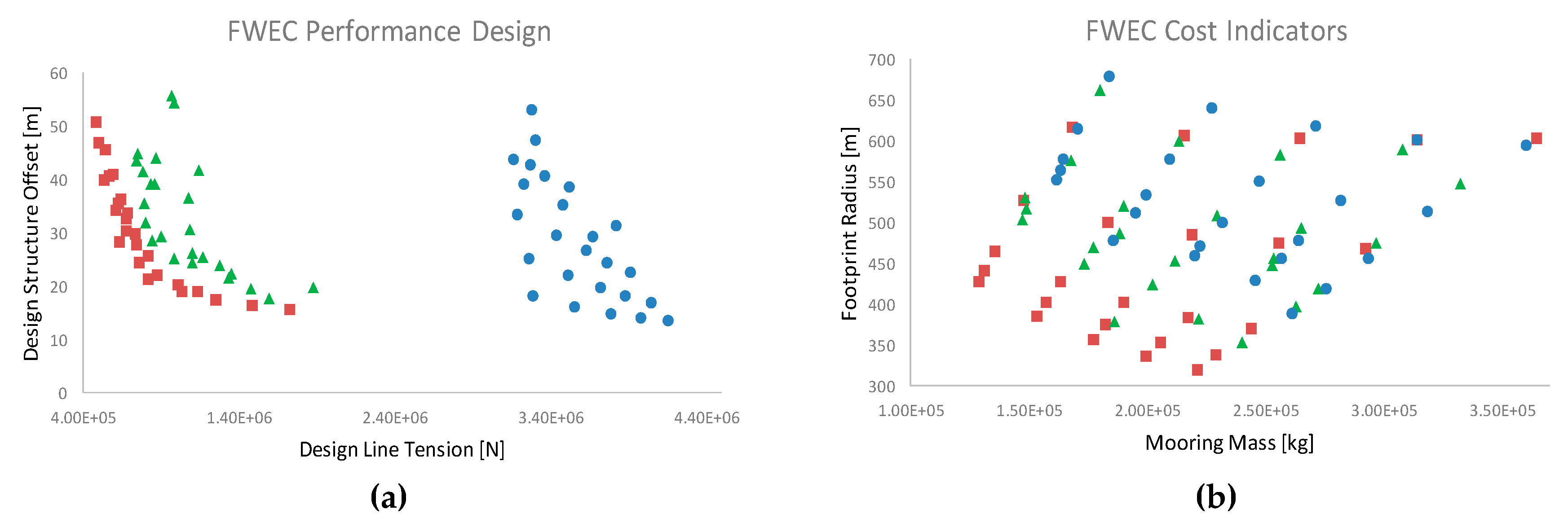
Figure 16.
Design (a) and cost (b) spaces for the FWEC structure with the QSFD (red squares), QSTD (green triangles), and DynTD (blue circles) models.
Figure 16.
Design (a) and cost (b) spaces for the FWEC structure with the QSFD (red squares), QSTD (green triangles), and DynTD (blue circles) models.
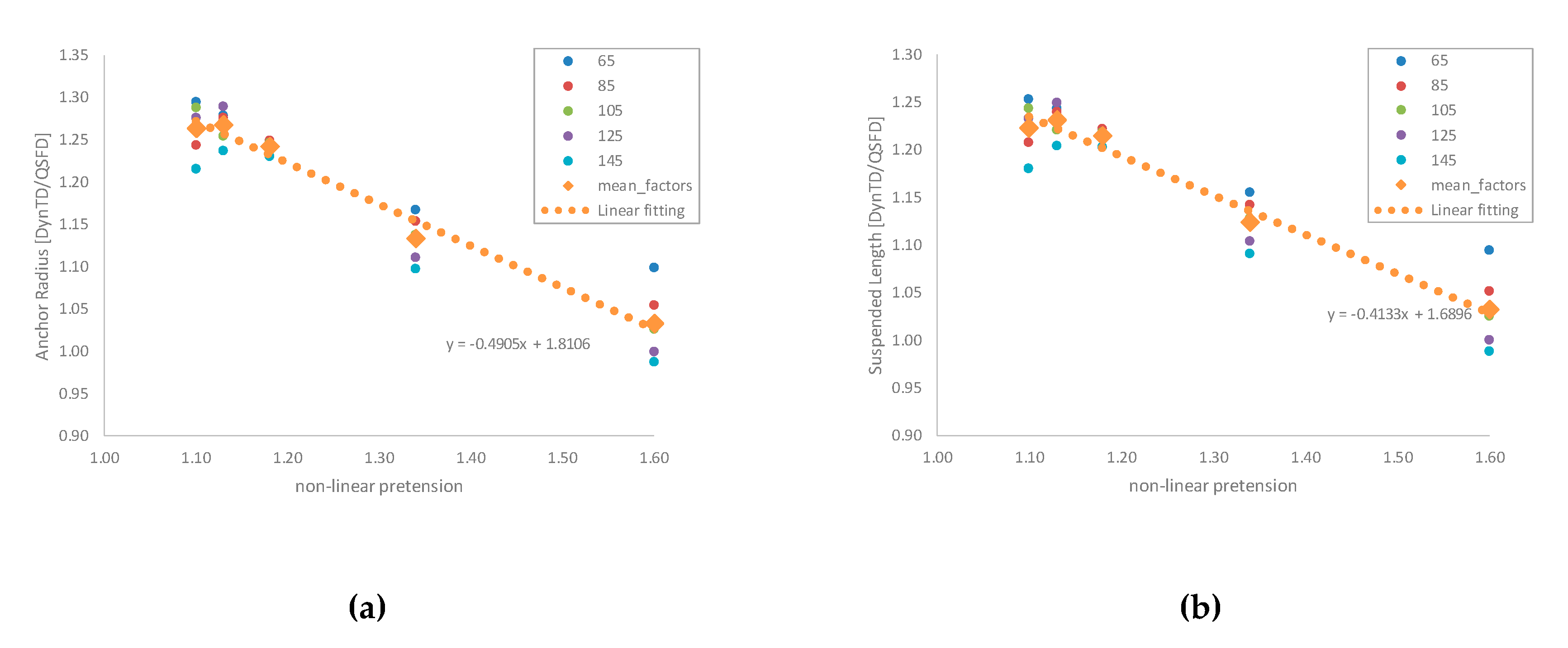
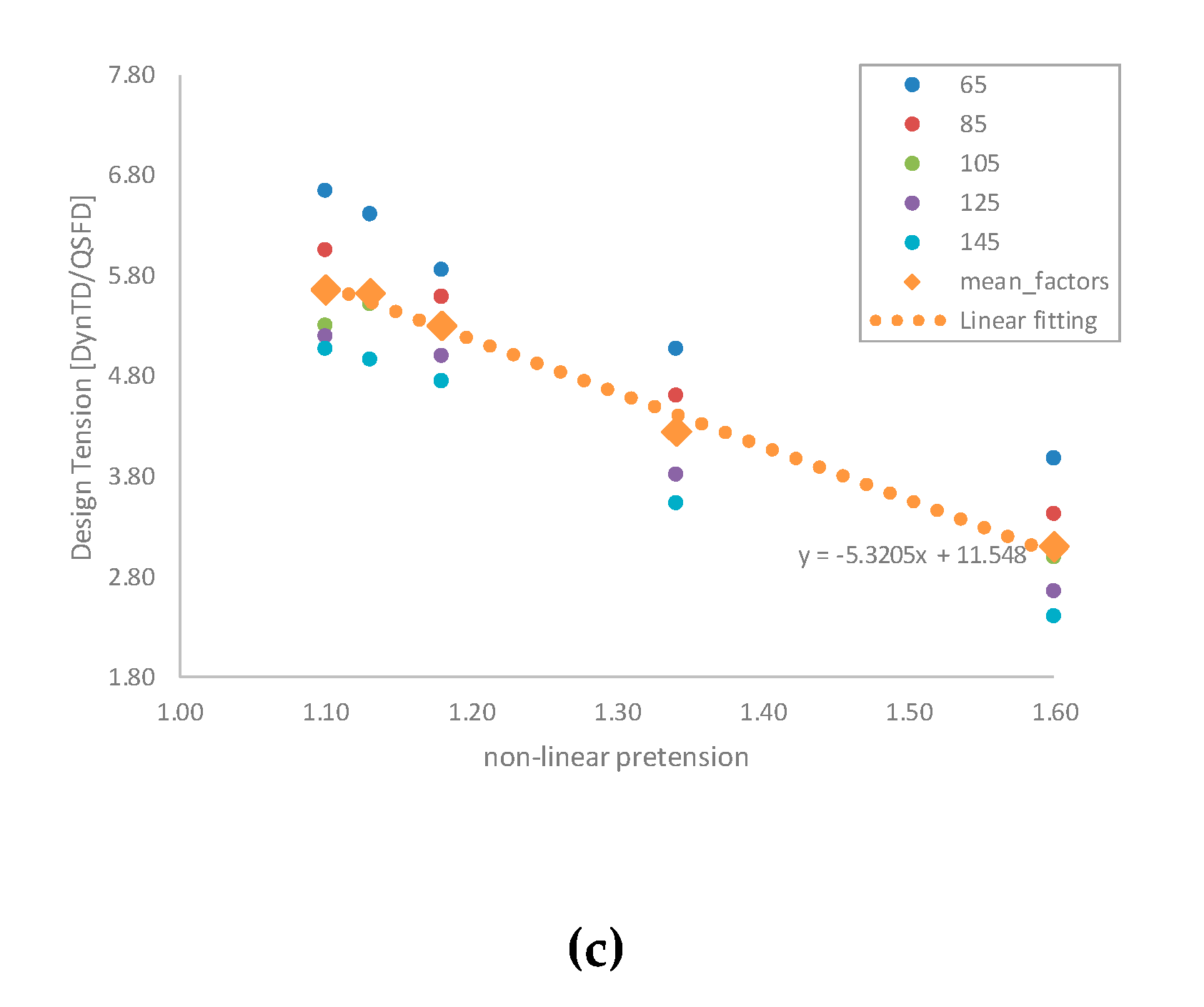
Figure 17.
Correction factors between the DynTd and the QSFD models for five linear mass values (65, 85, 105, 125, and 145) and a linear fitting of the mean values for Anchor Radius (a), Suspended length (b) and Design Tension (c).
Figure 17.
Correction factors between the DynTd and the QSFD models for five linear mass values (65, 85, 105, 125, and 145) and a linear fitting of the mean values for Anchor Radius (a), Suspended length (b) and Design Tension (c).
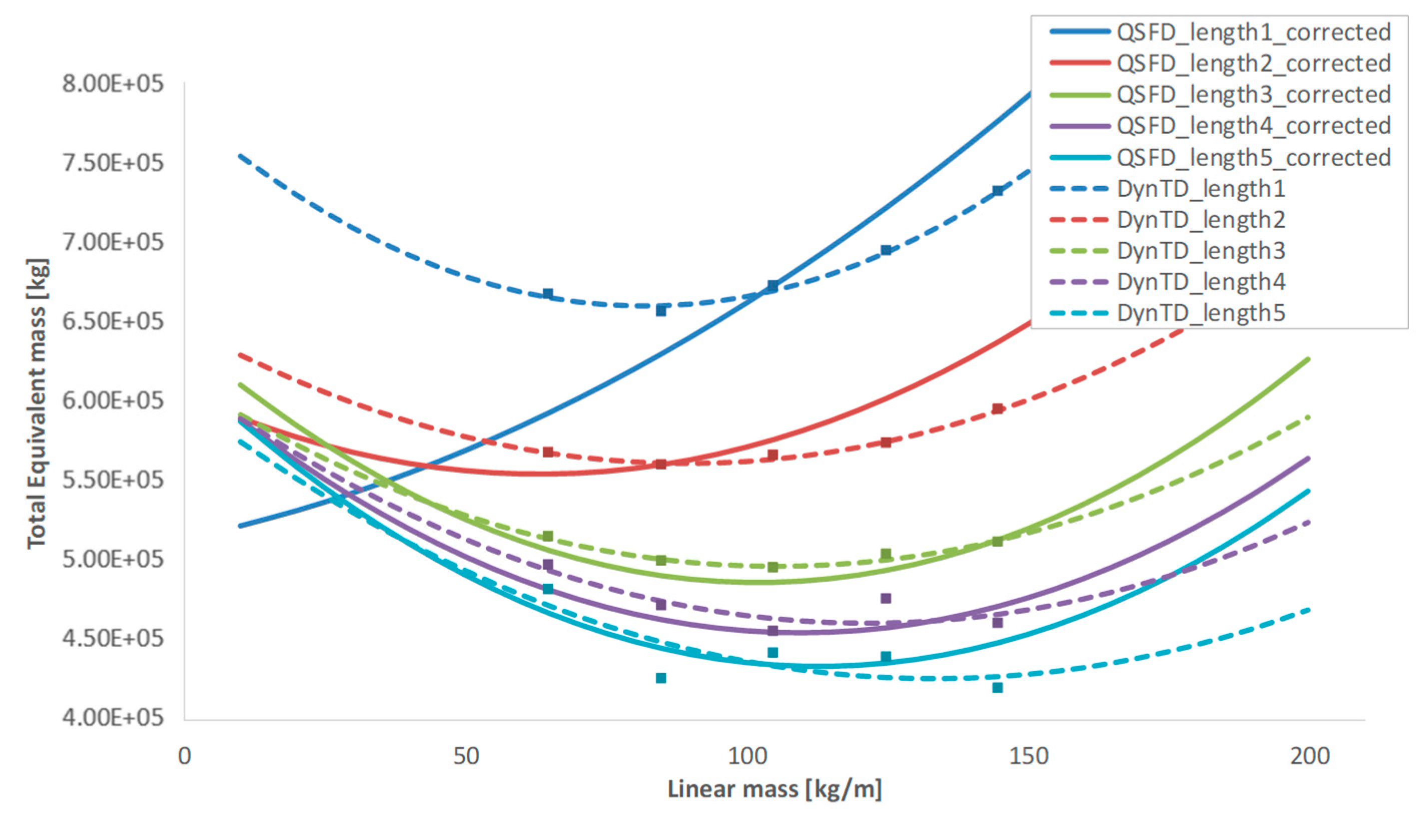
Figure 18.
Cost optimization of the mooring system. Total equivalent mass is the sum of 1/3 the lease area and the total mooring mass, assuming a cost ratio of 3 [€/kg]/[€/m2].
Figure 18.
Cost optimization of the mooring system. Total equivalent mass is the sum of 1/3 the lease area and the total mooring mass, assuming a cost ratio of 3 [€/kg]/[€/m2].
Table 1.
Environmental conditions for the reference simulation case.
Table 1.
Environmental conditions for the reference simulation case.
| Parameter | Return Period | Value |
|---|
| Significant Wave Height | 100 yrs | 10 m |
| Peak Period (Tp) | | 18 s |
| Current Velocity (Vc) | 50 yrs | 1.3 m/s |
Table 2.
Mooring properties selected to be combined for simulation cases, resulting in 25 cases arisen from combining each linear mass with each non-dimensional pretension.
Table 2.
Mooring properties selected to be combined for simulation cases, resulting in 25 cases arisen from combining each linear mass with each non-dimensional pretension.
| Mooring Linear Mass [kg/m] | Non-Dimensional Pretension [-] | Length/Mass Number |
|---|
| 65 | 1.43 | 1 |
| 85 | 1.26 | 2 |
| 105 | 1.16 | 3 |
| 125 | 1.10 | 4 |
| 145 | 1.06 | 5 |
Table 3.
Viscous force factors used for the FWEC.
Table 3.
Viscous force factors used for the FWEC.
| Degree of Freedom | Viscous Force Factor |
|---|
| Surge [N·s/m] | 1.188 × 10⁵ |
| Sway [N·s/m] | 1.188 × 10⁵ |
| Heave [N·s/m] | 4.469 × 10⁴ |
| Roll [N·m·s] | 3.532 × 10⁹ |
| Pitch [N·m·s] | 3.532 × 10⁹ |
| Yaw [N·m·s] | 0 |
Table 4.
Mean obtained kurtosis and skewness of the FWEC motions and tension of the most loaded line, obtained with the QSTD approach.
Table 4.
Mean obtained kurtosis and skewness of the FWEC motions and tension of the most loaded line, obtained with the QSTD approach.
| FWEC | Surge | Heave | Pitch | Mll Tension |
|---|
| Kurtosis (QSTD) | 2.924 | 2.671 | 2.241 | 3.700 |
| Skewness (QSTD) | −0.188 | −0.039 | −0.050 | 0.665 |
© 2020 by the authors. Licensee MDPI, Basel, Switzerland. This article is an open access article distributed under the terms and conditions of the Creative Commons Attribution (CC BY) license (http://creativecommons.org/licenses/by/4.0/).


