Article

MaRINET2 Tidal Energy Round Robin Tests—Performance Comparison of a Horizontal Axis Turbine Subjected to Combined Wave and Current Conditions

1
IFREMER, MetOcean Laboratory, 150 Quai Gambetta, 62 200 Boulogne-sur-mer, France
2
ESRU, Department of Mechanical & Aerospace Engineering, University of Strathclyde, James Weir Building, Montrose Street, Glasgow G1 1XJ, UK
3
CNR-INM, National Research Council, Marine Technology Research Institute, Via di Vallerano 139, 00128 Rome, Italy
4
FLOWAVE Ocean Energy Research Facility, University of Edinburgh, Max Born Crescent, Edinburgh EH9 3BF, UK
*
Author to whom correspondence should be addressed.
J. Mar. Sci. Eng. 2020, 8(6), 463; https://doi.org/10.3390/jmse8060463
Submission received: 25 May 2020 / Revised: 19 June 2020 / Accepted: 20 June 2020 / Published: 24 June 2020
(This article belongs to the Special Issue Marine Renewables–Infrastructures and Physical Testing)

Abstract

:
This Round Robin Test program aims to establish the influence of the combined wave and current effect on the power capture and performance of a generic tidal turbine prototype. Three facilities offering similar range of experimental conditions have been selected on the basis that their dimensions along with the rotor diameter of the turbine translate into low blockage ratio conditions. The performance of the turbine shows differences between the facilities up to 25% in terms of average power coefficient, depending on the wave and current cases. To prevent the flow velocity increasing these differences, the turbine performance coefficients have been systematically normalized using a time-average disc-integrated velocity, accounting for vertical gradients over the turbine swept area. Differences linked to blockage effects and turbulence characteristics between facilities are both responsible for 5 to 10% of the power coefficient gaps. The intrinsic differences between the tanks play a significant role as well. A first attempt is given to show how the wave-current interaction effects can be responsible for differences in the turbine performance. In these tanks, the simultaneous generation of wave and current is a key part often producing disruptions in both of these flow characteristics.

1. Introduction

Prototype testing is an integral part of the development process for many technologies. Testing at small scale can be relatively quick and inexpensive, while testing within a controlled environment enables experiments to be repeated for a range of different parameters. One of the main disadvantages associated with experimental research is related to the existence of side effects which could potentially lead to an inadequate interpretation of results. These uncertainties may be related to random or systematic errors which involve the test environment or the appliance. In the case of the performance evaluation of marine energy converters, the test environment may refer to facilities involving flume or tow tanks and the appliance usually refers to the converter and the instrumentation equipment to measure the variables of interest; for example, power, loads, and so forth.
A Round Robin Test (RRT) can be designed to enable a first stage quantification of a facility’s impact on the technology being tested and on the quality of the tests results. These results are obtained with the same testing program being repeatedly undertaken on the same device model and at a number of test laboratories, as performed by Aubrun et al. [1] on porous disc models representing wind turbines. As a consequence, better identification and quantification of the investigated causal factors can take place. In addition, such tests can be used to evaluate and improve (if necessary) the specifications given in the international standards—IEC TS 62600-200 to 202 [2,3,4], in the ITTC procedures and guidelines [5,6] or in the EquiMar protocols [7] for instance, as explained by Germain et al. [8,9].
To establish the influence of the test environment on the power capture and performance of a tidal turbine prototype, a first RRT has been undertaken during the FP7 MaRINET project by Gaurier et al. [10]. This programme consisted of testing the exact same 0.7 m diameter horizontal axis tidal turbine in four facilities—two tow tanks and two flume tanks. The turbine was tested at four flow speeds between 0.6 m/s and 1.2 m/s. Despite the fact that average values of power and thrust had small discrepancies, the time-fluctuating series showed larger differences which were related to turbulence in flumes and tow carriage vibrations from the tow tanks. More importantly, it was determined that the influence of blockage, even when this was in the order of ≃5%, influenced the performance of the turbine within operation ranges between peak power and free-wheeling. A blockage correction, for example, as proposed by Bahaj et al. [11], helps to improve the results comparison between facilities.
A similar analysis was undertaken by Murray et al. [12] where a horizontal axis turbine of 0.8 m was tested at a tow and a flume tank. As an addition to the work previously developed by Gaurier et al. [10], the comparative tests involved investigations related to the performance of two types of blade materials: composite and aluminium. The composite blades were specifically designed to enable bend and twist to facilitate load shedding while preserving optimal power output. Similar to the findings presented in Gaurier et al. [10], it was observed that torque and thrust average values increased slightly when the turbine was operating in the flume facility compared to the data obtained at the tow tank.
Understanding the impact that the extreme marine environment has on the survivability of tidal energy converters is fundamental for the successful development and commercialisation of full scale devices. Recent efforts from the scientific community to drive the development of tidal technology forward include the estimation of wave loading: for example, Gaurier et al. [13], Galloway et al. [14], Martinez et al. [15], Ordonez-Sanchez et al. [16] and Draycott et al. [17], or turbulence effects: for example, McNaughton et al. [18], Durán Medina et al. [19] and Gaurier et al. [20,21], on tidal energy devices. These investigations cover a wide range of topics ranging from the influences of diverse waveforms, wave directionality, control strategies or turbulent flow characteristics and intensities.
As demonstrated by Davies et al. [22] and Suzuki et al. [23], experimental modelling of the extreme loads tidal turbines are subjected to is necessary for blades or structure fatigue analysis. This experimental modelling requires an accurate inflow characterization with the wave and turbulence main parameters to be representative of full-scale conditions. However, such particular inflow conditions are (i) difficult to quantify because the wave and turbulence effects are sometimes difficult to separate [24] and (ii) difficult to re-create at model scale in experimental wave and current facilities [25]. That is the reason why the knowledge of wave and current characteristics in highly energetic sites is a real challenge. In order to reduce the research gap in this area, a Round Robin testing programme was conducted within the MaRINET 2 project which has received funding from the European Union’s Horizon 2020 research and innovation programme.
The aim of this work is to evaluate the potential difference, if any, when conducting combined wave and current trials on a generic marine turbine model in several towing and circulating tanks. In this paper, the three facilities used for this study are firstly described: the wave and current flume tank of IFREMER, the towing tank of CNR-INM and the FLOWAVE circular combined wave and current test tank. The generic model turbine is described before the presentation of the flow characteristics obtained in the three facilities. Finally, a comparison analysis of the turbine performance results is proposed and a discussion is given on several reasons which might explain some of the observed differences.

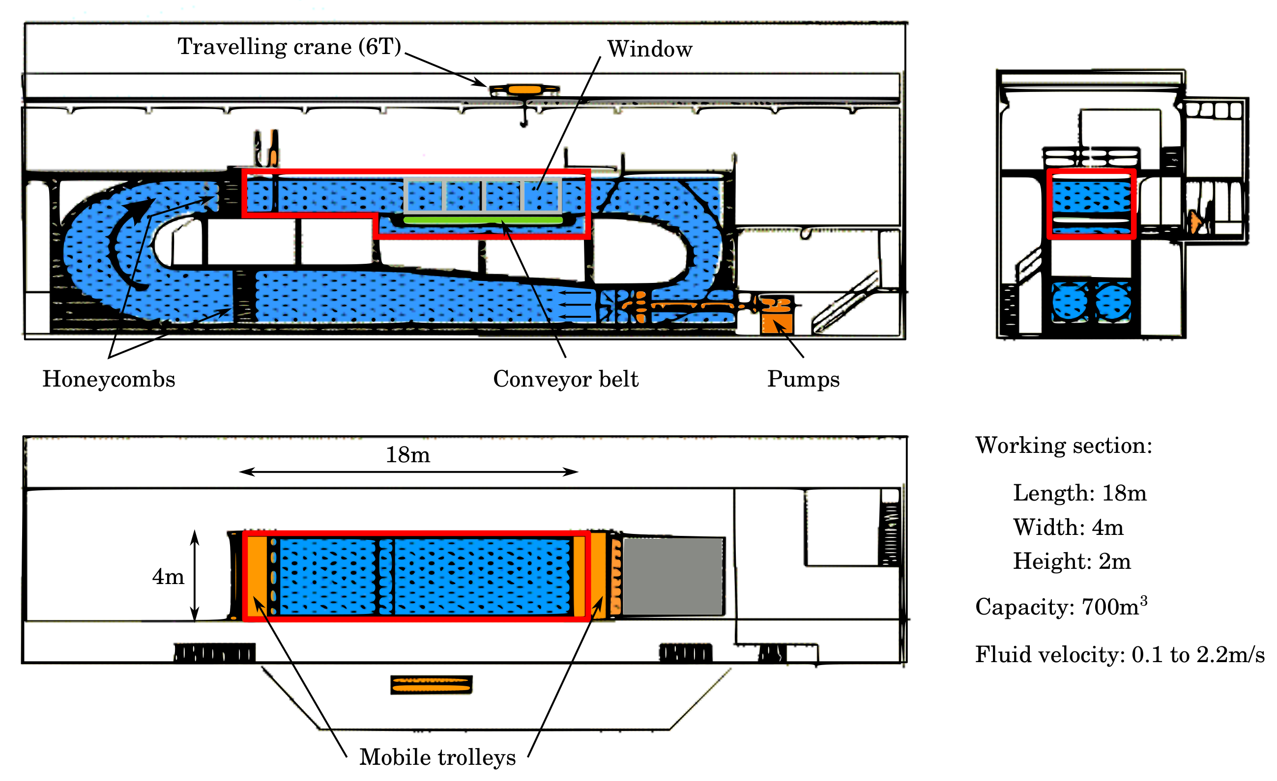
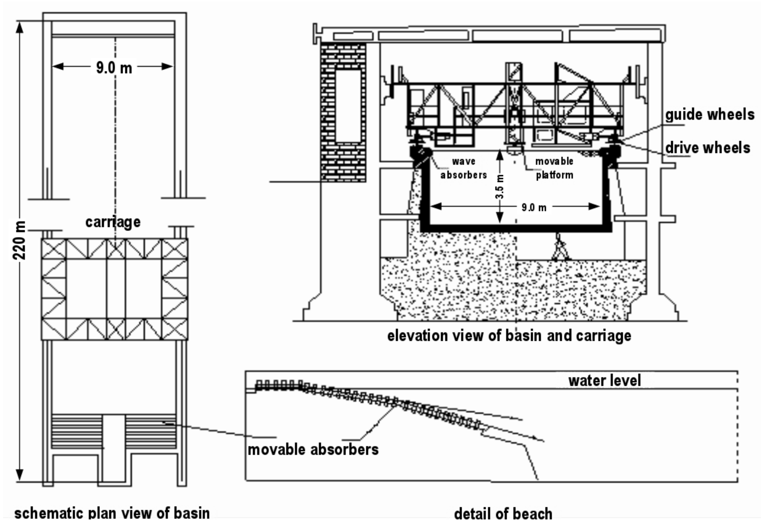
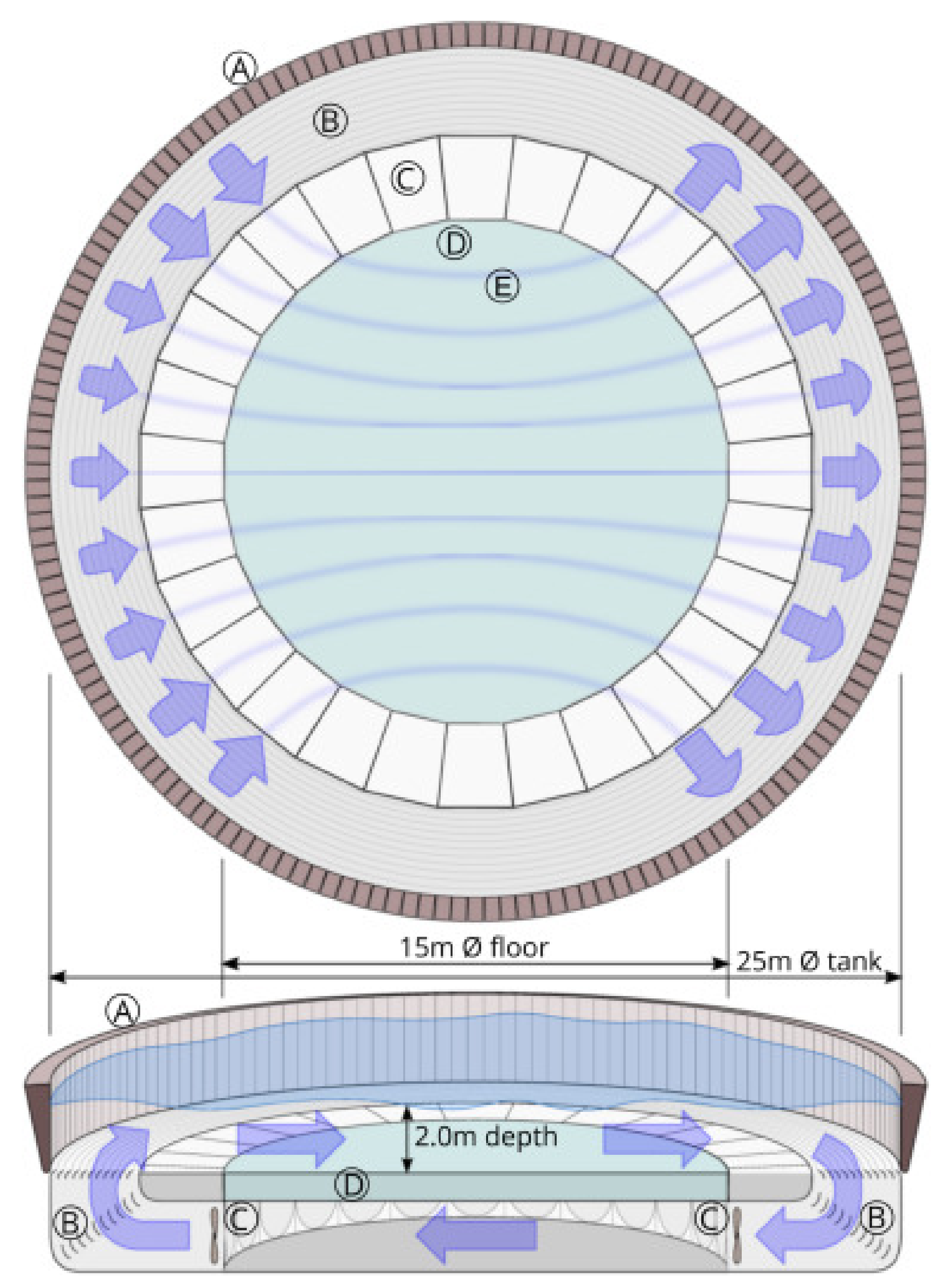
2. Experimental Set-Up

The first three sets of experiments of this Round Robin program were carried out at the circulating flume tank of IFREMER [26] (Figure 1), the tow tank of CNR-INM [27] (Figure 2) and the FLOWAVE circular combined wave and current test tank [28] (Figure 3) of the University of Edinburgh. These facilities were selected on the basis that their dimensions along with the rotor diameter of the turbine, D = 0.724 m, translate into low blockage ratio conditions, as seen in Table 1. The turbine was kept at a constant depth of 1.0 m and a variety of instruments to measure the flow conditions were mounted in close proximity to the turbine. Further details of the flow monitoring are presented in Section 2.3.
Additional details on the IFREMER and CNR-INM tanks can be found in the first RRT paper of Gaurier et al. [10] and in Sutherland et al. [28] for the FLOWAVE tank. The turbine was fixed on a moving carriage in the towing tank and on a customised mounting frame in both the flume tanks, as shown in Figure 4.

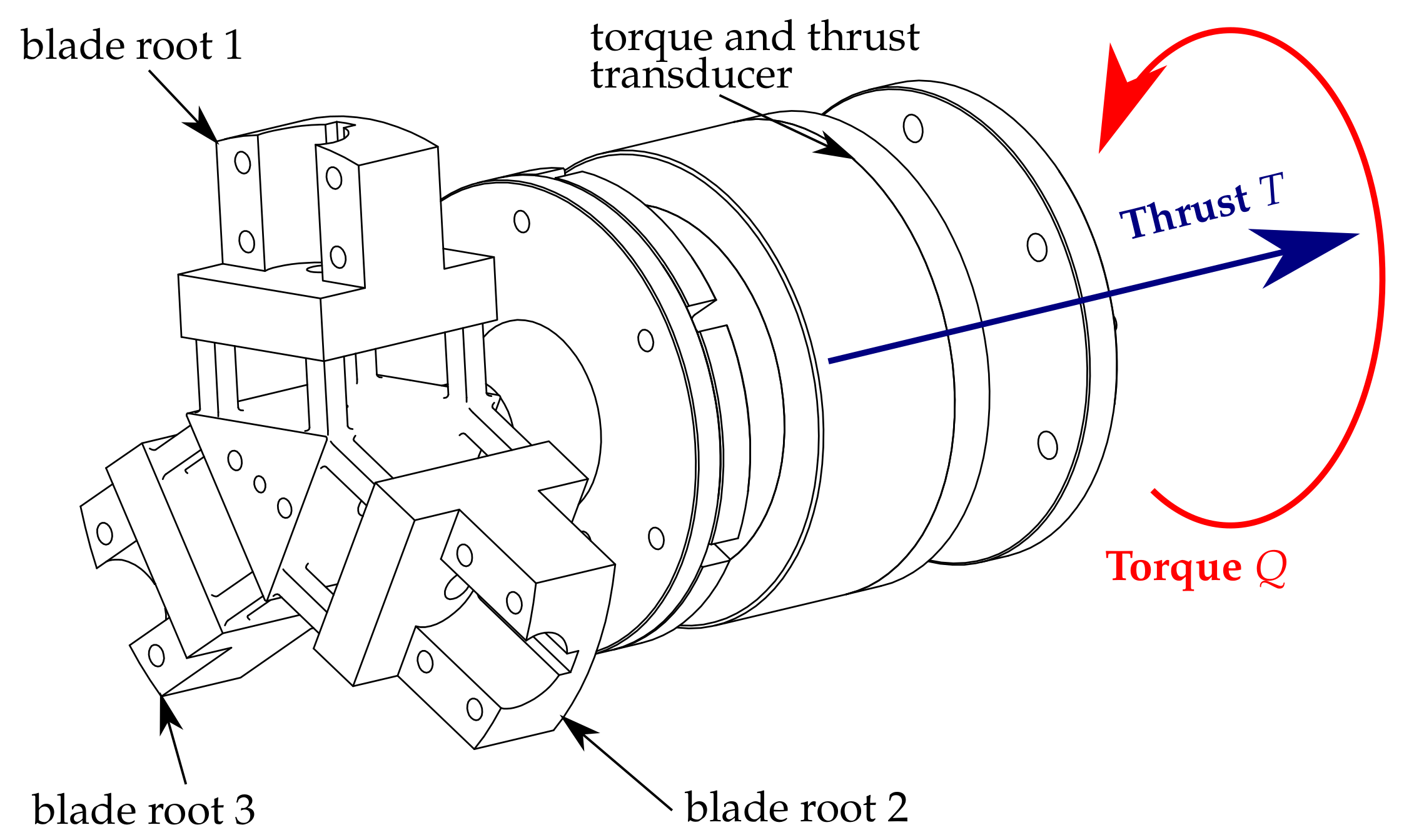
2.1. Turbine Prototype Specifications

A three bladed horizontal axis turbine developed by IFREMER is used in this RRT campaign. The turbine is 0.724 m in diameter (D) and a motor speed control unit is used to set various turbine rotational speeds. The blades were designed based on a NACA 63-418 profile and a full geometrical description is given in Gaurier et al. [10].
The generic turbine model is upgraded compared to the one used in Gaurier et al. [10], following the designed proposed by Payne et al. [29]. This advanced prototype is now equipped with a torque Q and thrust T transducer enabling these two main parameters applied to the rotor to be measured. This waterproof transducer (Figure 5) is positioned upstream of the seals of the machine to prevent measuring friction effects. This new transducer is custom made by the French company Sixaxes [30] in partnership with IFREMER. The measurement range is summarised in Table 2. The shielded cables coming from this transducer are routed through a slip-ring enabling the free rotation of the cables and prevent their entanglement. These low voltage signals are amplified by an electronic signal processing unit, located outside of the turbine and on the dry. The motor shaft is connected to the turbine shaft through a motor-gearbox (ratio 1:26) enabling suitable torque and rotation speed ratings.
All signals are acquired using National Instruments hardware and in-house electronics developed by IFREMER staff. The signals are sampled at a frequency ( f s ) of 128 Hz. Flow measurements and water surface elevation are also utilised and synchronised with the turbine instrumentations by means of a short impulse trigger signal.

2.2. Experimental Plan

The first part of the testing campaign including the turbine, comprises tests without wave interactions, thus the flow velocity or carriage velocity is set to 0.8 and 1.0 m/s until a full power curve has been established with at least ten points to construct the performance curves corresponding to the turbine. These curves are based on the non dimensional parameters: power coefficient C P and thrust coefficient C T , which are defined below:
C P = Q ω 0.5 ρ A U 3
C T = T 0.5 ρ A U 2
where Q is the mean hydrodynamic torque (in N·m) and T is the mean thrust (in N). The angular velocity of the turbine is represented by ω in rad/s. The turbine radius is R = D/2 = 0.362 m and A stands for the rotor swept area ( π R 2 ). The density of the water was considered in these calculations as 1000 kg/m 3 . Power and thrust coefficients are presented in relation to the Tip Speed Ratio ( T S R ). This non-dimensional value defines the ratio between the blade tip speed ( ω × R ) and the far upstream flow or tow velocity ( U ), as shown in Equation (3).
T S R = ω R U
The far upstream flow velocity U is estimated from measurements carried out without the turbine, but at the same position and when possible, for every tested flow condition, as explained in Section 2.3.
The second part of the testing protocol includes four regular waves in-line with the current: wave frequencies between 0.5 and 0.7 Hz and wave amplitudes between 35 and 75 mm and one irregular wave represented with a JONSWAP spectra, as presented in Table 3. The selection of these wave parameters (amplitude and frequency) was chosen based on the limitations set by each facility. However, considering a 1:20 scale and a Froude similitude, these correspond at some extent to a real site, with the following values: a current between 7.0 and 8.7 knots with wave heights between 1.4 and 3.0 m crest to trough and periods between 6.4 and 8.9 s, for a 14.5 m diameter turbine immersed in mid-depth of 40 m. At the model scale, the theoretical corresponding wavelengths are between 5.6 m and 7.0 m, which is far higher than the turbine diameter (D = 0.724 m). For each of the test cases eleven T S R were considered ranging from 0 to 7. To quantify the uncertainty of the experiment, repeated tests were considered for each case for several T S R . Due to time frame limitations and/or laboratory capabilities at CNR-INM and FLOWAVE, the test matrix was constricted to five T S R per case and two T S R for the repeated tests at CNR-INM and test case 5 was not carried out in FLOWAVE.

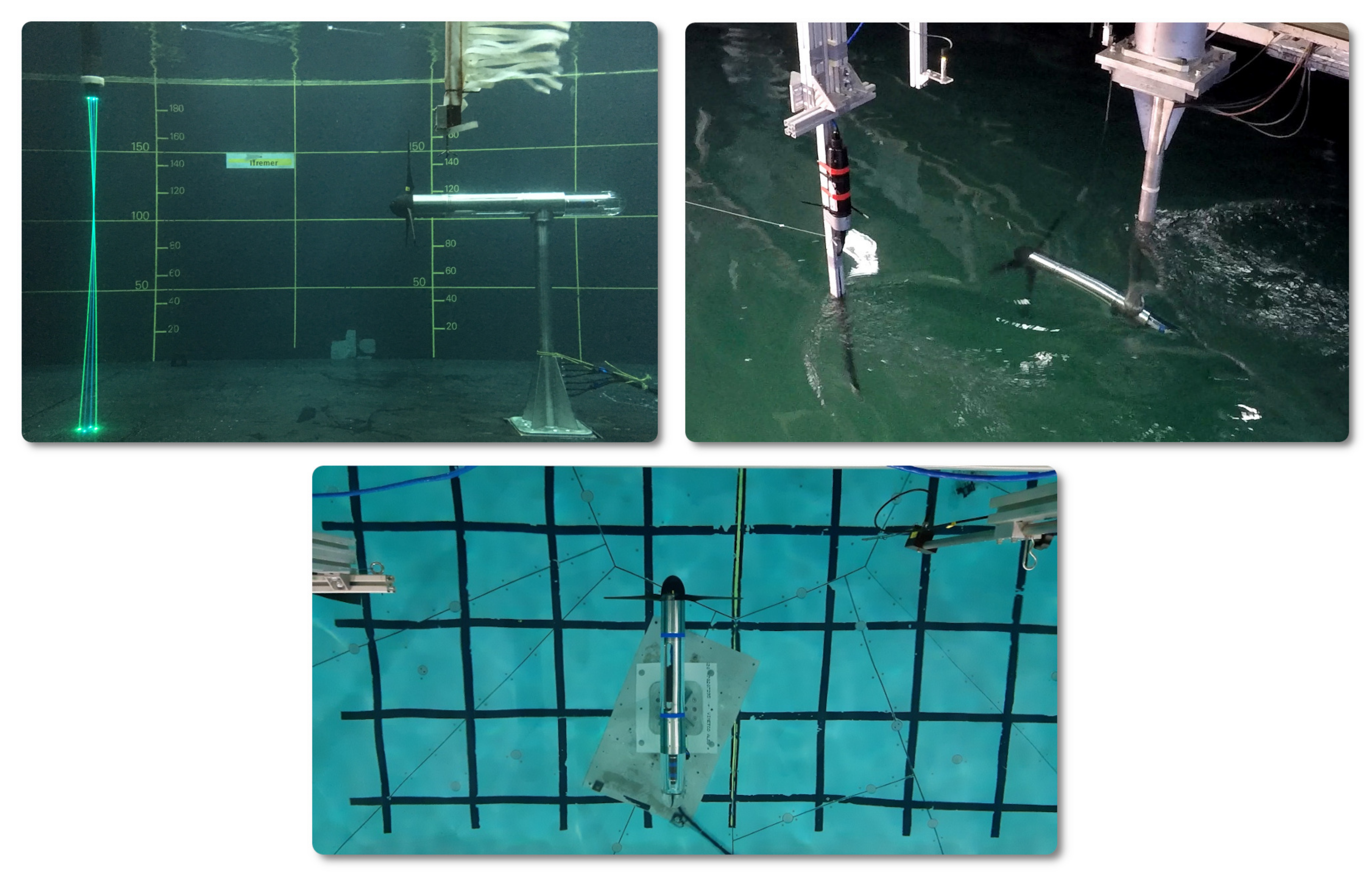
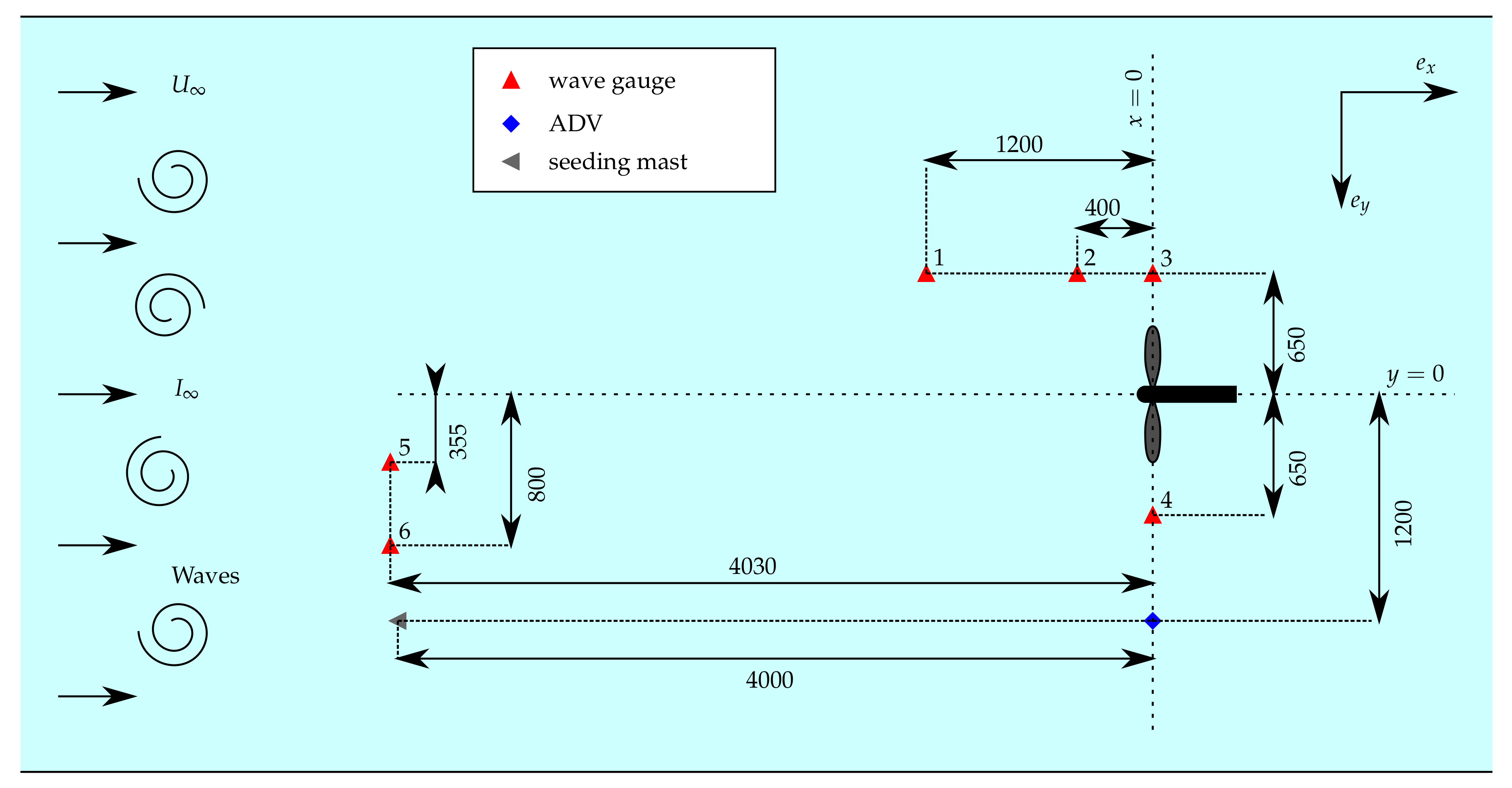
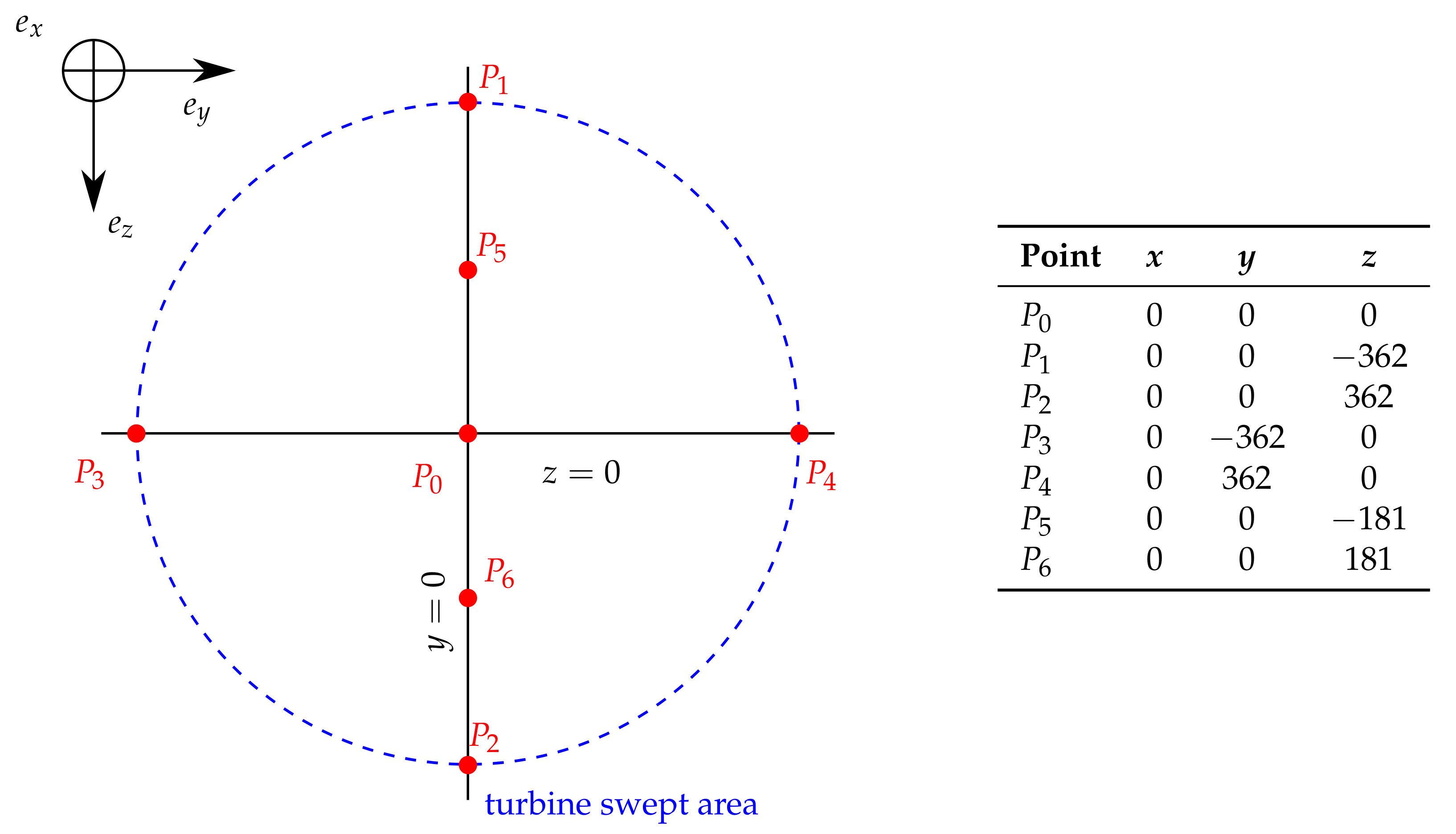
2.3. Flow Measurement and Characterisation

The flow stream is measured while the turbine is in operation using an Acoustic Doppler Velocimeter (ADV). The ADV is placed in line with the turbine hub at a distance of 1.2 m along the cross section of the tank (see Figure 6). At IFREMER and FLOWAVE, seeding particles are deposited in the tanks and continuous flow circulation permits a uniform dispersion in the flow stream. For the experiments at CNR-INM, a seeding mast is placed 4.0 m upfront of the ADV, in order to ensure a good measurement quality.
A number of wave probes are placed next to the turbine to measure the wave parameters set for each of the case scenarios. Three resistive wave probes are used at IFREMER and FLOWAVE: probes 1–3 as seen in Figure 6. A mix of resistive, ultrasound and dynamic wave probes are used in the CNR-INM tow tank: probes 3–6 as seen in Figure 6, where probes 4 and 6 are ultrasound wave gauges and probe 5 is a dynamic wave gauge. One single identical resistive wave probe is used in all facilities (probe 3). This is a crucial aspect of the test campaign, especially since the flow characteristics affected by the addition of waves is deemed to be relevant between facilities.
The flow stream is characterized in each of the facility without the turbine and for every generated wave and current flow condition. During these tests, ADV and wave gauges only are used in synchronization. The position of the ADV is adjusted to be exactly that of the turbine when operated, that is, at x = 0 . Depending on the facility, 3 or 5 ADV measurement points among the 7 displayed on Figure 7 are acquired over the turbine swept area in order to quantify a potential vertical or lateral velocity gradient: points P 0 , P 1 , P 2 , P 5 and P 6 are acquired at IFREMER, points P 0 , P 1 and P 2 are acquired at CNR-INM and points P 0 , P 1 , P 2 , P 3 and P 4 are acquired at FLOWAVE. These records are then processed to define the incoming (far upstream) velocity U required in Formulas (1)–(3). Results obtained during this flow characterization are presented and discussed in the following section.

3. Input Flow Characteristics

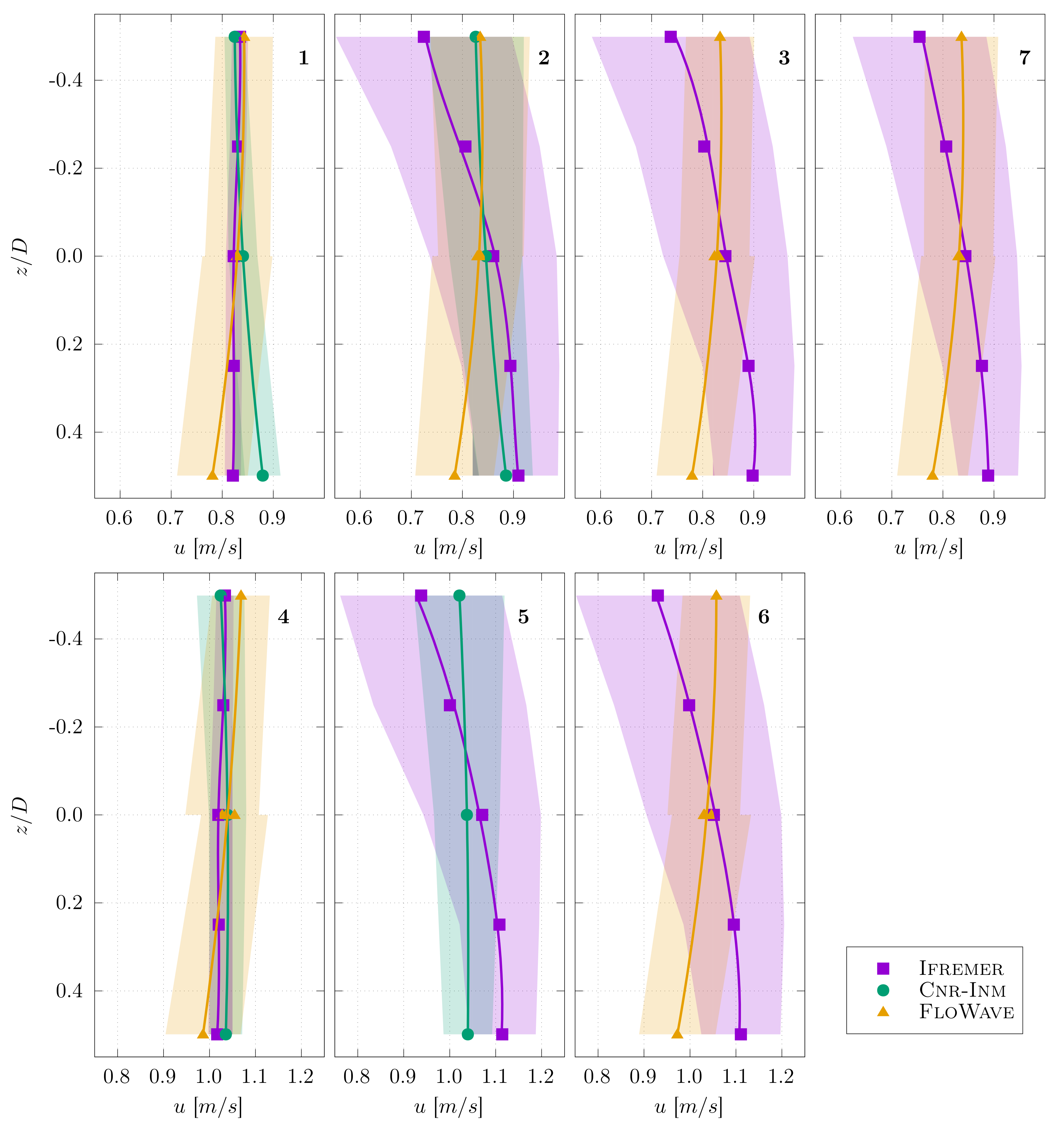
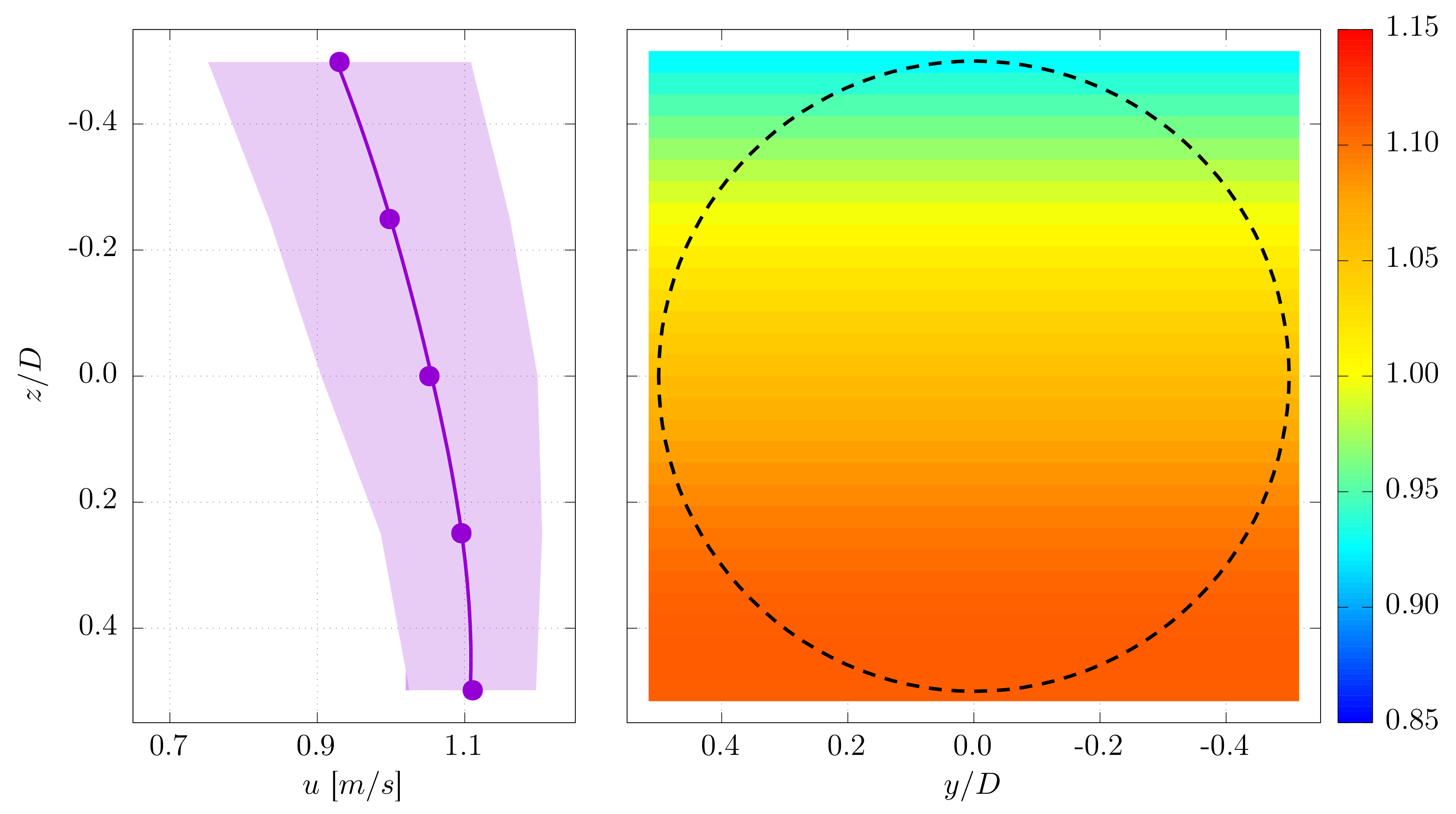
3.1. Flow Velocity Characterisation

Velocity measurements are carried out in each of the testing facilities and for every tested case (see Table 3) in order to characterize the flow perceived by the turbine. All these acquisitions are carried out without the turbine, but at the same position when operated. Figure 8 show the time average and standard-deviation of the stream-wise component of the velocity u. As seen on Figure 7, the vertical discretization of the profiles are composed of five depth points at IFREMER and three depth points at CNR-INM and FLOWAVE, between z / D = 0.5 and z / D = 0.5 , corresponding to the equivalent blades highest and lowest extremities respectively. For the FLOWAVE tank, two additional points are recorded on the sides, that is, z = 0 but y / D = [ 0.5 ; 0.5 ] . These two last points are plotted together at z = 0 on Figure 8.
Some cases are missing, mainly results coming from CNR-INM for cases 3, 7 and 6. This is mainly due to time constraints achieved at that facility which required extensive downtimes to achieve water settlement after wave testing; hence the authors decided to choose specific cases. One case is missing for FLOWAVE as well (case 5) because amplitudes of the wave at 0.7 Hz created with a flow of 1 m/s were too low. Due to the irrelevance of the test conditions, this case was omitted during the experiment and in consequence for the analysis.
The Goring & Nikora [31] de-spiking method has systematically been applied on every ADV record. Profiles presented for current-only cases (1 and 4) are quite linear and vertical for all tanks. The average shown for the deepest point ( z / D = 0.5 ) and case 1 at CNR-INM is different from the other facilities. This disparity can be associated to aliasing of the Doppler signal which is displayed as a series of spikes in the discrete signals. This happens again for the same depth and the same tank, for case 2. For these two particular records, the time average and standard-deviation seem to be affected when this is compared to the profile obtained for case 4. For the FLOWAVE tank, the deepest point shows a slightly lower average value. This is the same for every other tested case. For this particular tank, the standard-deviation is the highest for the current-only cases. Standard-deviation coloured areas profiles presented for this tank show a discontinuity at the depth z = 0 . This minor disparity is related to 3 measurement records ( y / D = [ 0.5 ; 0 ; 0.5 ] ) that were undertaken across the turbine section. For most of cases, these three points are quite similar meaning there is no horizontal shear in this tank, along the turbine diameter.
Velocity profiles displayed for the wave and current cases are significantly different from the current-only profiles, especially for the IFREMER tank. Wave and current profiles recorded in the IFREMER tank are not linear with the depth: a vertical gradient is visible on all profiles with the lowest average velocity at the top and the highest ones at the bottom. The difference can reach 0.2 m/s between the highest and lowest points depending on the cases. In parallel, the standard-deviation increases from the bottom to the top. This is due to the wave orbital velocities as well as to the fluctuations coming from the presence of the wavemaker in the flow, at the entry of the test section. For the CNR-INM towing tank, average profiles are vertical again and their standard-deviation increase from the bottom to the top, due to the wave orbital velocities. At the FLOWAVE tank, velocity profiles are quite similar between cases with the lowest velocities at z / D = 0.5 and with a constant standard-deviation with the depth.
With such vertical gradients on the average profile velocities, using the central measurement point (at z = 0 ) as the inflow velocity U is not accurate enough, especially in a tank comparison point of view. For this reason, a disc-integrated method is proposed in this study to account for the vertical variations of the velocity perceived by the turbine, as described by Mycek et al. [32]. A spline curve fits the ADV measurement points for each profile, as depicted by the violet curve on Figure 9 for case 6 at IFREMER flume tank. Then, this spline is extended along the transverse y dimension and the disc-integrated average is processed over the turbine diameter (the dashed black line). In addition, a particular attention is paid to the processing of the velocity average for thrust and power coefficients—the square or cubing of the velocity is processed prior to temporal and spatial averaging, as demonstrated by Blackmore et al. [33].
In the following, the disc-integrated velocity is systematically applied in the Formulas (1)–(3). This procedure is justified given two main considerations:
  • It accounts for the velocity gradient over the entire turbine disc. The hypothesis about a constant velocity along the transverse dimension y is at least confirmed by the measurements carried out at FLOWAVE, where the central point ( z = 0 ) is repeated for three different transverse positions: y / D = [ 0.5 ; 0 ; 0.5 ] , and results show a similar average velocity. Identical measurements have been carried out at IFREMER for previous trials showing the same results. At the towing tank of CNR-INM, the transversal velocity variation is null and thus, this approach does not alter the final velocity distribution.
  • There is no turbine effects linked to the momentum theory on the velocity measurement because the acquisition is carried out without the turbine, but at the same location.
Results obtained with this method are summarized in Table 4 as mean values of U , for all the test cases and the three tanks. As explained previously, some cases were discarded during the testing campaigns and these are indicated with NA. To relate power and loadings to the inflow parameters for all the cases, a similar corresponding velocity value is chosen when this information is unavailable; for example at CNR-INM for test case 3, the value obtained for test case 2 is used (same velocity with waves).
As it can be seen in Table 4, the velocity magnitudes acquired in each of the facilities are within the same order of magnitude. They are all slightly higher than the requested velocities (0.8 m/s and 1.0 m/s) by at least 2 cm/s. Differences appear however on velocity averages measured at the IFREMER flume between cases with or without wave: 2.2 cm/s between cases 1 and 2 and 3.2 cm/s between cases 4 and 5. On the contrary, results are closer in the other tanks, with a maximum difference of 5 mm/s between cases 1 and 2 at CNR-INM and cases 2 and 3 or 4 and 6 at FLOWAVE. The larger differences observed at IFREMER between cases with or without wave is due to the previously noticed sheared and turbulent velocity profiles when positioning the wavemaker into the tank, creating a blockage in the upper section of the water column.
Span-wise velocity components v and w are presented in Figure 10 and mostly for the data generated at the mid-hub section ( z = 0 ) and for points P 0 , P 3 and P 4 , when available. The average velocity of these components is lower than 1 cm/s for every case and facility. However, these values are globally slightly positive for v and negative for w. These average tendencies can be explained by slight misalignments of the ADV probe in the tanks.
Standard-deviation is globally higher for the wave and current cases, because of the wave orbital velocities and higher fluctuations. These variations are not clear for the FLOWAVE data, where the turbulence seems to dominate the fluctuating part of the velocity. The CNR-INM standard-deviations are particularly high for the v component and for cases 4 and 5 because of transverse vibrations of the ADV probe for 1 m/s velocity.
The turbulence intensity is displayed on Figure 11 for the same points. The classical Formula (4) is used to process the 3 dimensional turbulence rate ( σ stands for standard-deviation).
I 3 D = 100 × 1 3 σ ( u ) 2 + σ ( v ) 2 + σ ( w ) 2 u ¯ 2 + v ¯ 2 + w ¯ 2 .
The wave frequency component has been filtered and removed from the velocity measurements for all the wave and current tests, before processing the standard-deviation. So, the wave orbital velocities have not been accounted in these turbulence rate results. According to Figure 11, the turbulence intensity is between 2 and 16% for all cases and tanks. For FLOWAVE, the turbulence is quite constant, with values between 6 and 8% depending on the cases. For IFREMER, the current-only cases (1 and 4) show values lower than 2%, whereas for current and wave conditions the turbulence rate reaches 8% or higher. Finally, values obtained at CNR-INM are widely distributed with relatively high values. These values are higher than 14% for cases 4 and 5, that is, with flow velocity of 1 m/s. This results is explained by the ADV probe vibrations already observed on the large standard-deviation of the v component of the velocity on Figure 10.

3.2. The Wave Effects

For current and wave cases, the previously shown standard-deviation includes the wave orbital velocity component as well as the turbulence of the flow in the flume tanks. To separate and quantify the periodic part of this fluctuation linked to the wave, the Hilbert transform u ^ ( t ) of the stream-wise component of the velocity u ( t ) is processed using Formula (5).
u ^ ( t ) = 1 π u ( τ ) t τ d τ .
With this definition, u ( t ) and u ^ ( t ) form the complex conjugate pair and the analytic signal Z ( t ) can be introduced as:
Z ( t ) = u ( t ) + i u ^ ( t ) = a ( t ) e i θ ( t ) ,
in which:
a ( t ) = u ( t ) 2 + u ^ ( t ) 2 and θ ( t ) = arctan u ^ ( t ) u ( t ) .
As explained by Huang et al. [34], the polar coordinate expression of Equation (6) further clarifies the local nature of this representation: it is the best local fit of an amplitude and phase varying trigonometric function to u ( t ) . The magnitude a ( t ) of the analytic signal Z ( t ) is the instantaneous envelope of the original signal u ( t ) and θ ( t ) is its instantaneous phase. This last Equation (7) is used to process the envelope a ( t ) and its time-average and standard-deviation are presented on Figure 12.
Results obtained at IFREMER are different from those measured at FLOWAVE or CNR-INM—average and standard-deviation of the amplitude of the Hilbert transform are larger compared to the other tanks. These large values indicate a higher amplitude as well as a higher variation of the waves created in this tank. In addition, these waves are combined with a turbulent flow in the wake of the wavemaker, characterized by low frequency flow-induced variations, included in the amplitude of the Hilbert transform.
For the FLOWAVE tank, the average and the standard-deviation of the amplitude appear to be quite constant with the depth. For case 2 however, the velocity amplitude can be higher than 0.1 m/s, especially for z > 0 . For every other case, the average amplitude is lower than 0.1 m/s and the standard-deviation is about 0.05 m/s.
The two cases tested at CNR-INM show an increase of the average amplitude of the velocity from the bottom to the top, with values between 0.05 m/s and 0.13 m/s. The standard-deviation stays however low and constant with depth, indicating a low variation of the wave orbital velocity with time.
The larger amplitude of the periodic component of the velocity observed at IFREMER are confirmed by the analysis of the surface elevation measured by the wave gauge at the turbine position and displayed on Figure 13. The same method is applied to the wave gauge measurements—that is, the Hilbert transform is processed and the time average and standard-deviation of its amplitude are displayed.
For all the regular wave cases (2, 3, 5 and 6), wave amplitudes are higher at IFREMER compared to the other facilities and to the requested ones (Table 3). It is the contrary at FLOWAVE where the wave amplitudes are lower or equal than the requested parameters. For these two flume tank, because waves are created with the current, wave amplitudes are reduced and this effect needs to be accounted. Depending on the tank, this effect may be differently managed and compensated. For the two tested cases carried out in CNR-INM, the wave amplitudes correspond to the requested ones.
As for the velocity amplitude, the highest standard-deviation of the surface elevation is reached at IFREMER for all tested cases. This parameter stays quite low in the two other tanks, excepted for case 7 because of the irregular wave.

4. Performance Comparisons

As explained in the previous section, the velocity U is processed from the characterization of the inflow measured at the same position of the turbine (without the turbine). The disc-integrated method and the square or cubing of the velocity prior to temporal and spatial averaging enable an accurate processing of the power and thrust coefficients (Formulas (1) and (2)). These performance coefficients are shown and compared among the tanks and the cases in this section.

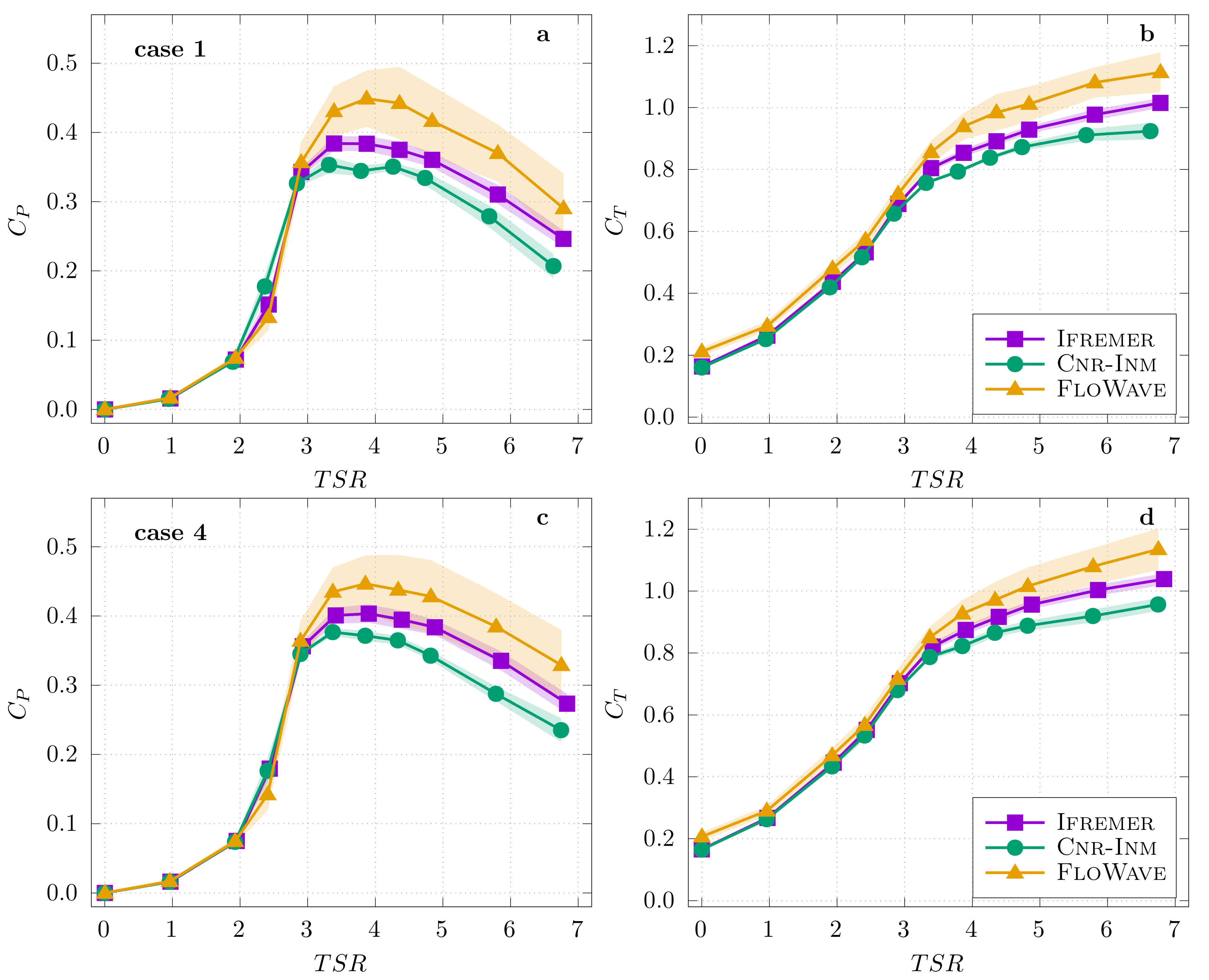
4.1. Turbine Performance Comparison with Current-Only

For the current-only cases (1 and 4), the power and thrust coefficients are displayed on Figure 14. Average performance as well as standard-deviation are presented on this figure for both flow velocities 0.8 m/s and 1.0 m/s. First of all, these results are quite similar in terms of curve tendency. However, a gap between the curves clearly appears from T S R > 3 —highest values are obtained in the FLOWAVE tank (yellow curves) as well as the highest standard-deviations. For the power coefficient (Figure 14a,c), the maximum difference between the tanks represents about 25% between CNR-INM (green curve) and FLOWAVE (yellow curve) at T S R = 4 . Concerning the thrust coefficient (Figure 14b,d), this maximum difference is reached for the highest T S R and is about 20% between the same two tanks. In terms of C P , the maximum values are higher or equal to 0.45 for T S R 4 . This maximum value is 0.38–0.40 at IFREMER (violet curve) and 0.35–0.37 at CNR-INM (green curve), with the highest values reached for case 4, that is, for the highest flow velocity of 1.0 m/s. This slight increase of the C P curve with the flow velocity is already mentioned in Gaurier et al. [10] as a Reynolds effect.
Similarly, the standard-deviation is twice as high for the results obtained at FLOWAVE compared to the others facilities. This last remark corresponds to the velocity profiles already observed on Figure 8, where the standard-deviation of the measured velocity for cases 1 and 4 is about twice as high in FLOWAVE compared to the same profiles obtained in the other tanks. The natural turbulence of the flow in FLOWAVE (Figure 11) explains such a large standard-deviation. With a lower gap, the standard-deviation is globally lower at CNR-INM (green curve) compared to IFREMER (violet curve), which is visible as well on the C P curves (Figure 14a,c), especially for 4 < T S R < 5 . This difference in terms of natural turbulence intensities between the tanks can partly explain the difference between the average coefficients—as already observed by Blackmore et al. [33], an increase of the turbulence characteristics can slightly increase the performance of the turbine.

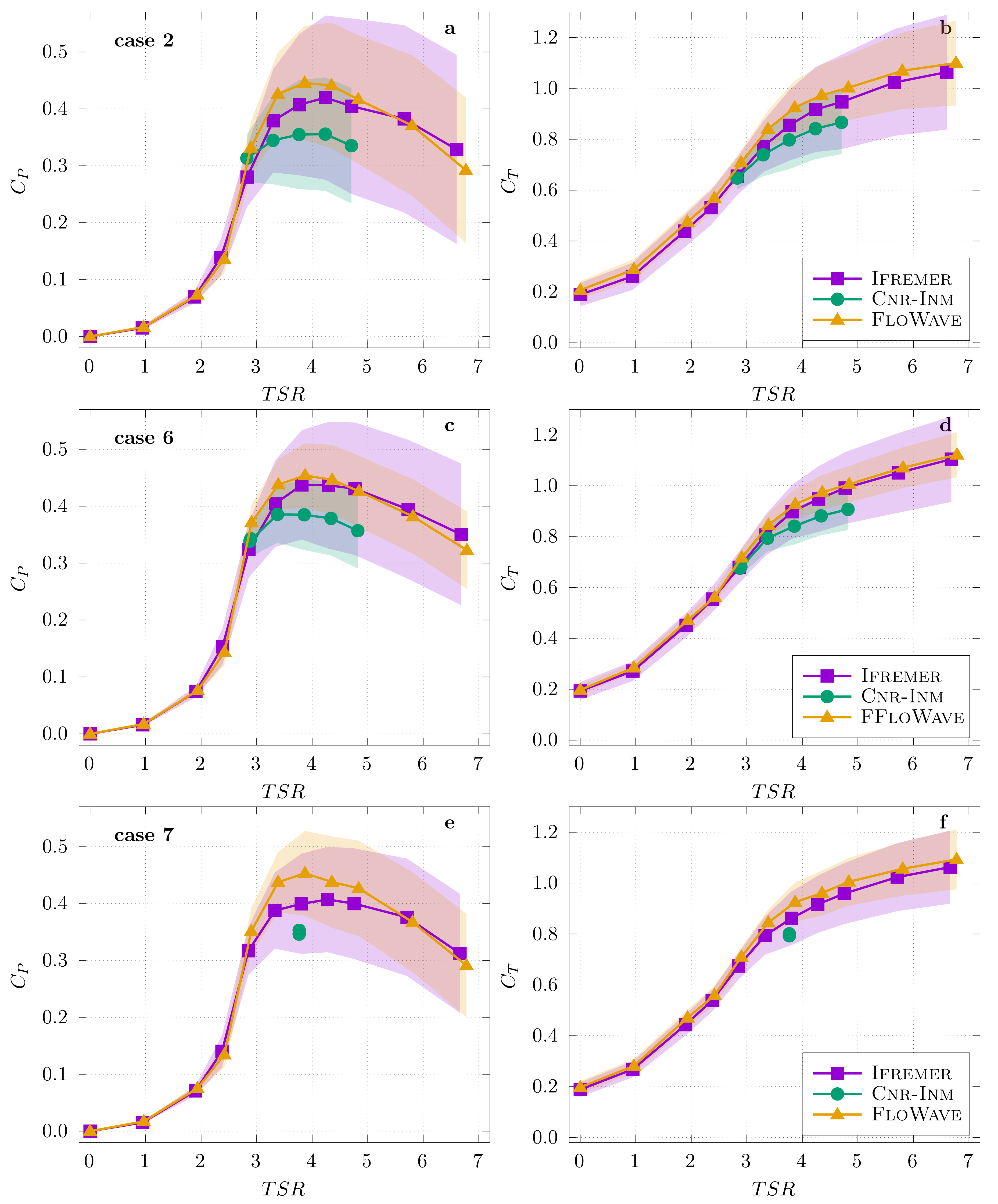
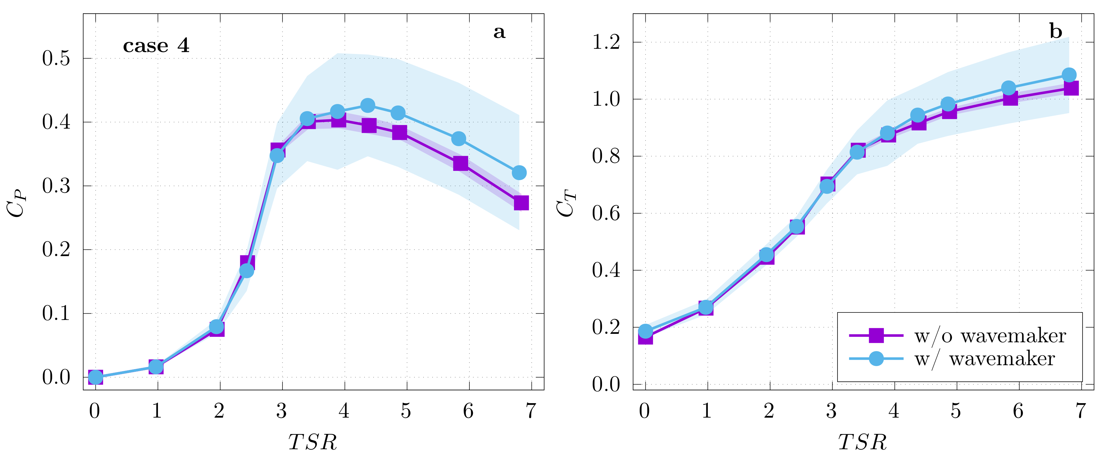
4.2. Turbine Performance Comparison with Current and Wave Conditions

Performing the same processing on the wave and current conditions leads to Figure 15 where results from cases 2, 6 and 7 are presented for flow velocities of 0.8 m/s and 1.0 m/s and regular or irregular waves, and for all the three tanks. Please note that these results are also displayed within an individual test site on Figure A1 for an easier comparison.
These curves are in relatively good agreement, especially for IFREMER and FLOWAVE results (violet and yellow curves), on the contrary to what is shown on Figure 14 for current-only cases. As already mentioned previously, the wavemaker at IFREMER is intrusive and increases the turbulence rate. As previously shown on Figure 11, the turbulence intensity in the tank of IFREMER is then higher than the one measured at FLOWAVE. This is directly visible in the standard-deviation part of the curves, with the highest values observed for C P and C T in the IFREMER flume tank. However, the turbulence is not the only explanation for this high standard-deviation—as mentioned in the previous section, the average wave amplitude is higher in this tank compared to the others from about 10 mm in CNR-INM to about 40 mm in FLOWAVE depending on the cases (see Figure 13). As a consequence, the amplitude of the periodic fluctuating part of the velocity is higher at IFREMER compared to the other tanks (as depicted on Figure 12). Such fluctuations in the velocity directly increase the standard-deviation of the turbine performance coefficients.
Power and thrust coefficients measured at CNR-INM are always lower or equal to those obtained at IFREMER or FLOWAVE (green versus violet and yellow curves on Figure 15): between 0.35 and 0.38 for C P and T S R = 4 at CNR-INM and between 0.40 and 0.45 for the same parameters at IFREMER and FLOWAVE. The blockage ratio, which is 5 times higher at IFREMER compared to CNR-INM, as observed in Table 1, may be an explanation for such a difference. However, this ratio is also very close between CNR-INM and FLOWAVE despite significant differences in their turbine performance results. This blockage effect is consequently not the only one explanation. It is further discussed in Section 5.1. The velocity fluctuations which are higher for the flume tanks of IFREMER and FLOWAVE compared to CNR-INM may be another explanation. Only considering the results obtained at IFREMER showing the largest variations between the cases as depicted by Figure A1, the highest turbine performance is measured for case 6. According to Figure 12, the amplitude of the orbital velocity in this tank is 0.15 m/s for case 2, 0.17 m/s for case 6 and 0.12 m/s for case 7, at z / D = 0 . The turbulence rates measured for the same corresponding cases are quite identical with 9%, 10% and 9.5% respectively (Figure 11). For the turbine power coefficient, that finally leads to C P ¯ = 0.41 , 0.44 and 0.40 (Figure 15a,c,e), respectively for cases 2, 6 and 7 and for T S R = 4 . The highest performance is then obtained for the highest amplitude of the velocity fluctuations, wherever those fluctuations come from the periodic wave orbital velocities or the turbulent velocity fluctuations. These velocity fluctuations are consequently another explanation for the lower performance coefficients obtained at CNR-INM compared to IFREMER or FLOWAVE. The turbulence effects are further discussed in Section 5.2.
Finally, only considering the turbine performance measured at CNR-INM and FLOWAVE (green versus yellow curves), average results are very close to those obtained for current-only cases (see Figure A1 as well). The main significant difference concerns the standard-deviation of these coefficients which are higher for the wave and current cases. For example, for T S R = 4 , σ ( C P ) = 0.10 for case 2 and σ ( C P ) = 0.06 for case 6 in both tanks, whereas the same parameter is σ ( C P ) = 0.01 at CNR-INM and σ ( C P ) = 0.04 at FLOWAVE, for cases 1 and 4 (without wave). The standard-deviation is then multiplied by 1.5 to 2.5 for FLOWAVE and by 6 to 10 for CNR-INM, between cases without and with waves. This difference in the increase of the standard-deviation of the turbine performance between the tanks can be explained by the flow turbulence already perceived by the turbine at FLOWAVE for the current-only cases, creating some fluctuations in the turbine measurements. When adding the wave to the current, the standard-deviation of these measurements increases again, due to the periodic wave orbital velocities and their interactions with the current, explaining the multiplier coefficients of 1.5 to 2.5. However, these coefficients are smaller for FLOWAVE compared to the same results at CNR-INM (6 to 10), because the fluctuations perceived by the turbine for the current-only tests in this tank are very low, due to the intrinsic characteristics of the towing tank, that is, without turbulence. In addition, the wave and current interactions occur at FLOWAVE (as well as at IFREMER) and can explain a different behaviour of the turbine compared to CNR-INM. This last point is further discussed in Section 5.3.

5. Discussion

In the previous section, some differences have been noticed between the turbine performance results obtained in the three tanks. The amplitude of these differences can reach 25% depending on the cases. These differences are mainly related to the different flow characteristics generated in the three tanks, as shown on Section 3 and discussed in Section 4.

5.1. Blockage Effects

The blockage ratio is 5 times higher at IFREMER than at CNR-INM or FLOWAVE (see Table 1) and it is essential to account for this parameter for turbine performance evaluation. In Gaurier et al. [10], authors used the method proposed by Bahaj et al. [11] to compensate for blockage effect differences. Applying the same method on the actual results leads to the blockage correction factor ( U T / U F ) 3 depicted on Figure 16 to be applied to the power coefficient.
These correction factors are slightly different from the ones presented in Gaurier et al. [10]: for example, for the IFREMER flume tank at T S R = 4 , ( U T / U F ) 3 = 0.93 , 3% lower than the value quantified for the previous study. These coefficients are based on the relative size of the facility compared to the turbine diameter and on the measured thrust coefficient. Here, the turbine diameter is slightly larger than in the previous study ( D = 0.724 m instead of D = 0.700 m) however this small gap does not explain such a difference. During the previous RRT, the thrust was not measured on the turbine rotor, but from a load-cell based on the top part of the supporting mast. In order to remove the drag part from the mast, authors subtracted the drag measured at T S R = 0 to the one measured at every other T S R . With this new turbine model, the thrust is now measured directly from the rotor, thus minimising errors related to measurement techniques.
The CNR-INM and IFREMER curves in Figure 16 follow a similar trend but with a difference in amplitude, explained by variations in the cross sectional areas of both facilities. Results obtained at FLOWAVE are however different, especially for T S R > 5 . These very last points show even lower values than those obtained for IFREMER. Contrary to the typical facilities, the FLOWAVE tank has a circular shape and therefore, quantifying the cross section is somewhat difficult to determine. For this study, the equivalent usable length of this tank (15 m as shown in Table 1) was considered as the total width. However this might not be the optimum choice, given two main factors:
  • The turbine cannot be located exactly in the mid-position of the tank due to the floor mounting design. Thus, it is likely that distances to the surrounding walls differ from either side.
  • The depth of the tank (2 m) is relatively small compared to the tank diameter. Thus, the depth could be predominant in terms of blockage for the turbine.
Applying these correction factors to the turbine performance curves leads to Figure 17 for cases 4 and 6. The blockage correction improves some of the curves, for example, decreasing the difference between CNR-INM and IFREMER for the current-only case 4. For the same case 4, the turbine power coefficient measured at FLOWAVE for T S R = 4 is still 13% different than from those obtained at CNR-INM and IFREMER. Furthermore, results measured at the IFREMER flume tank are still slightly higher than those from the CNR-INM towing tank for wave and current case 6 and for T S R > 3.5 . In addition, for the same wave and current case 6, results between FLOWAVE and IFREMER are very similar without correction (Figure 15) whereas they are quite different with the blockage correction here. Finally, the blockage correction method presented in Bahaj et al. [11] accounts for the tank section area, which can be problematic to define for a circular tank like FLOWAVE. In this study the actual tank diameter is taken as reference width, but this choice is questionable, since it is not supported by blockage correction models specific for circular tanks. For the wave and current cases, the blockage correction is not sufficient to explain the encountered differences between turbine performance measured in the tanks. Other parameters including turbulence and wave generation could be attributed to the result disparity.

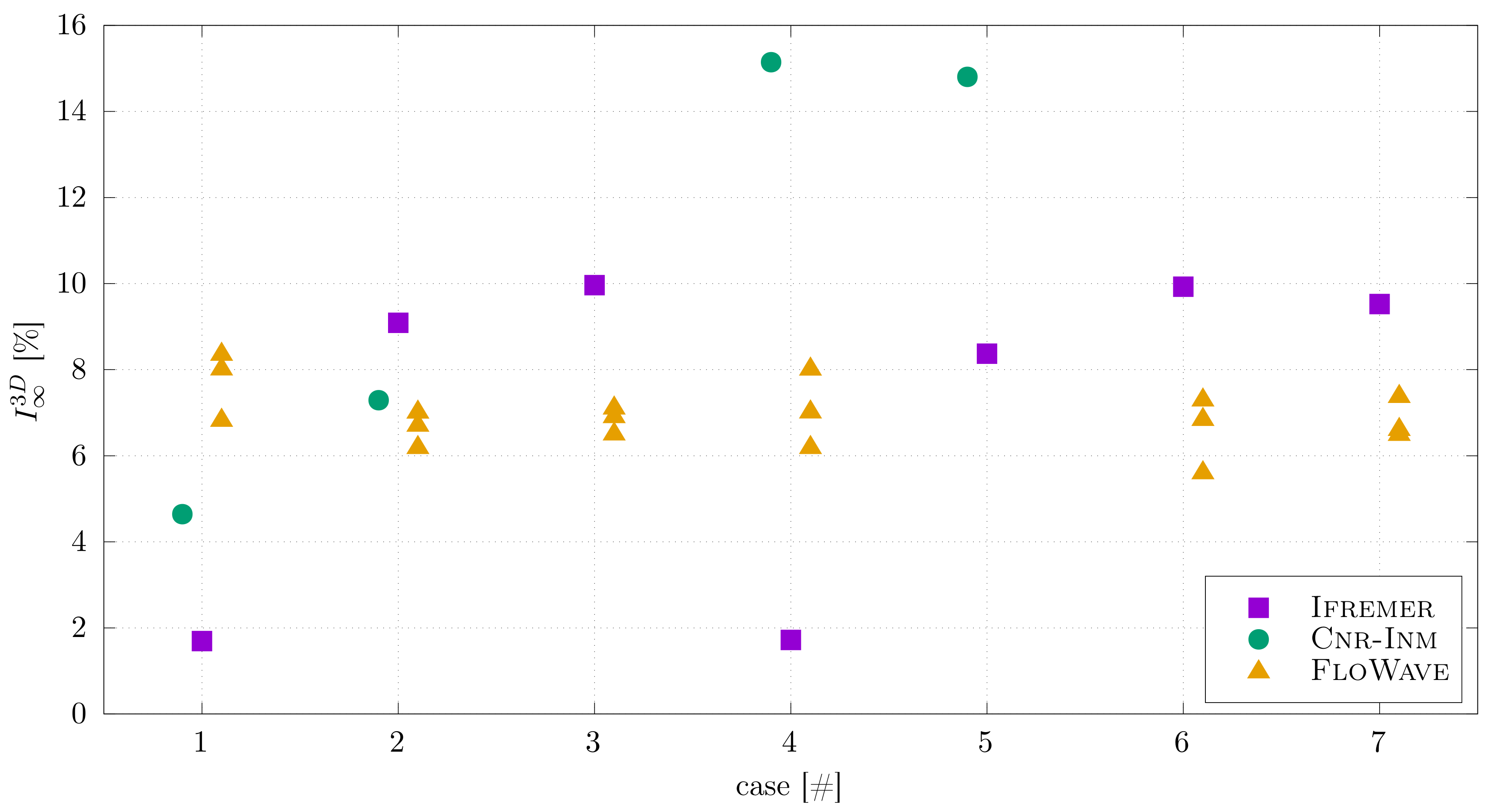
5.2. Turbulence Effects

As shown by Blackmore et al. [33], an increase of the flow turbulence characteristics can slightly increase the turbine performance and associated fluctuations. This turbulence effect has been tested only at IFREMER, where the wavemaker is a separate feature of the facility; that is, it can be added or removed from the facility. Without the presence of the wavemaker, the turbulence rate is I 2 % as depicted on Figure 11 for cases 1 and 4. With the presence of the wavemaker, the turbulence rate increases to I 8 % as the flow outlet is constrained by the bulky wavemaker. In this additional study, the two cases are studied: the operation of the turbine in the flume without wavemaker and with the wavemarker in position but inoperative (parked). Results are displayed in Figure 18 comparing the performance of the turbine operating at 1 m/s at low turbulence level (without wavemaker, case 4) and with higher turbulence rate (with parked wavemaker). The same exact data processing is performed for both cases.
According to these results, the presence of the parked wavemaker increases the turbine performance for T S R 4 . For the power coefficient, the increase of the time-average amplitude is about 8% at T S R = 4.4 . The standard-deviation significantly increases as well for both coefficients after T S R = 3 : for example, for T S R = 4 , σ ( C P ) is about 7 times higher with the parked wavemaker than to case 4 (without wavemaker).
Consequently, the turbulence effects can partially explain the difference observed in the power coefficient curves between FLOWAVE and CNR-INM/IFREMER for case 4 noticed on Figure 17, after accounting for the blockage ratio. As remarked previously, this difference is about 13% which is however higher than the effects of the turbulence observed at IFREMER previously (Figure 18) which is limited to 8%. Furthermore, these turbulence effects do not explain the difference between the power coefficient curves obtained at IFREMER and FLOWAVE for case 6 on Figure 17. These two last curves are processed from measurements carried out in quite a similar turbulent flow (Figure 11), but the results are still different by 3.5% for T S R = 4 after accounting for the blockage ratio: C P = 0.422 at FLOWAVE and C P = 0.407 at IFREMER. The wave and current interactions may explain such a difference.

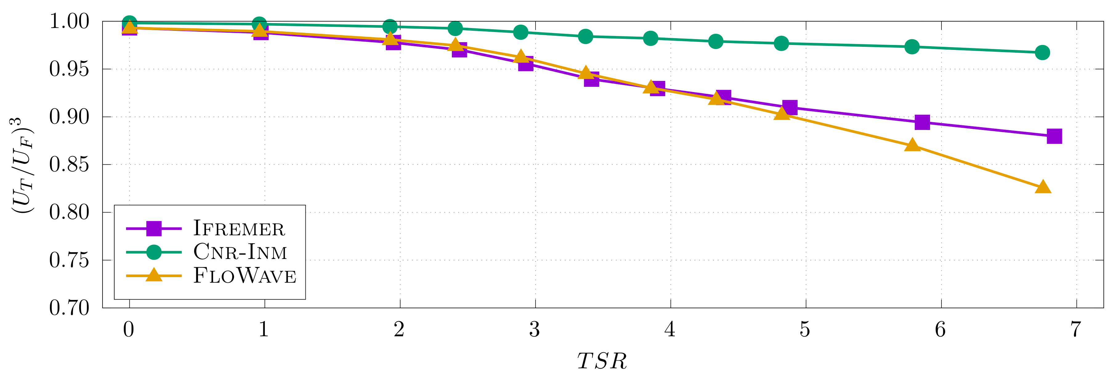
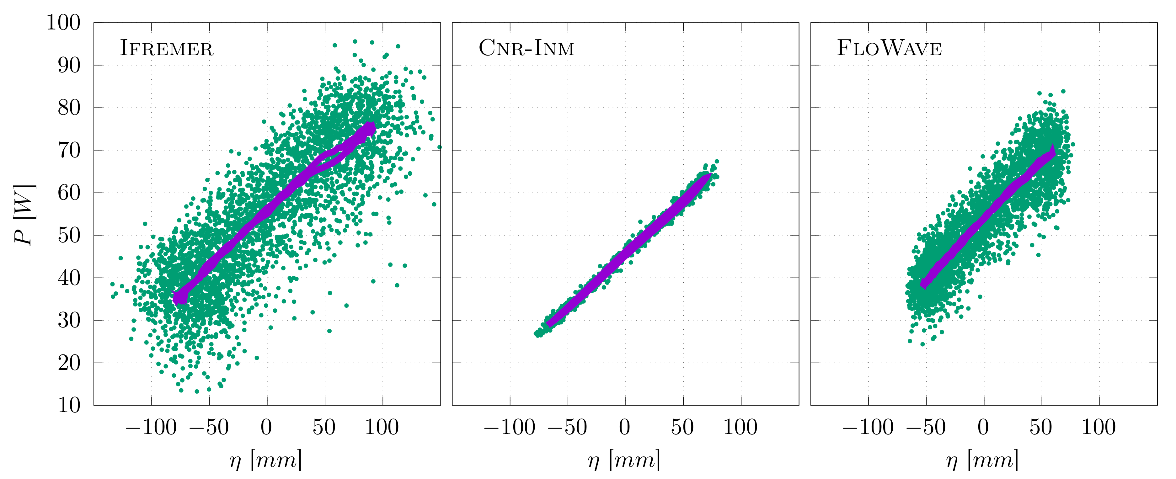
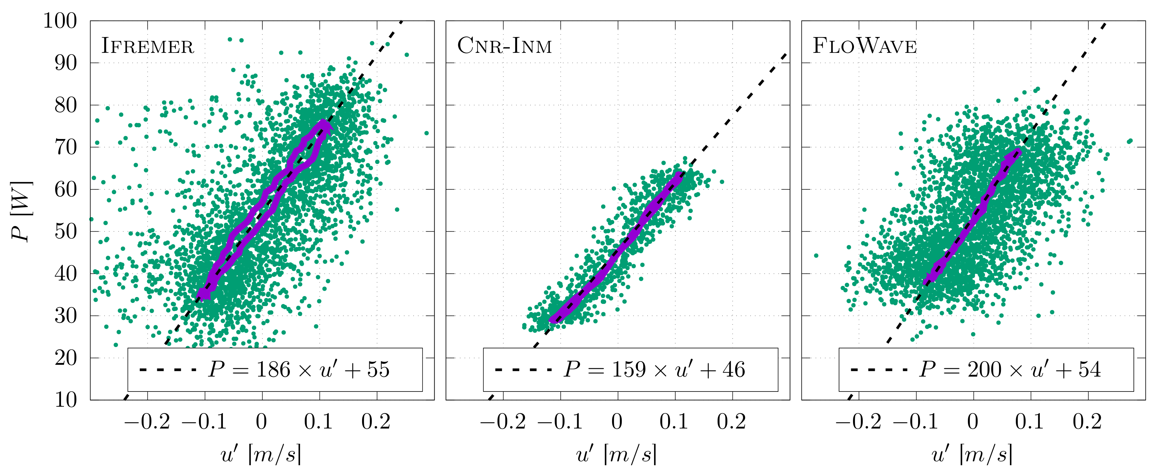
5.3. Wave and Current Interaction Effects

The wave and current interaction effects are not as easy as the turbulence or blockage effects to consider. It has been common knowledge for several years that current modifies wave amplitude and length and also, wave changes the vertical velocity profile. Brevik and Bjørn [35] carried out some experimental tests in 1979 with various waves and currents and compared their results to the theory. Klopman et al. [36] performed intensive tests in a wave and current flume tank on that subject, clearly showing these effects. To the authors’ knowledge however, this particular non-linear interaction applied on a marine turbine has never been compared. These type of experiment requires the same equipment tested at non interacting environments (towing tank) and where interactions can not be dismissive (flume tank).
Such a comparison can be done from this experimental campaign, using the flow velocity (ADV) and wave amplitude (wave probe 3) measurements acquired in synchronisation with the turbine performance and both located at the rotor plane (Figure 6). As a first attempt, a comparison was made for the results obtained for T S R = 4 on the wave and current case 2, between the three selected tanks. To visualize the wave and current effect on the turbine power production better, the same presentation proposed by Guo et al. [37] is picked out and displayed on Figure 19 and Figure 20, respectively versus the water level η and the velocity fluctuations u .
From these results and especially from the raw data (green points), it is first clearly noticeable that the wave amplitude variations are much higher in the flume tanks of IFREMER and FLOWAVE compared to the towing tank of CNR-INM. Consequently, the velocity fluctuations are higher as well in the same tanks. This corresponds to the results shown on Figure 12 and Figure 13. The wave phase average of these raw data, depicted by the violet curve, globally shows the same trend between the three tanks with a maximum of the turbine power production corresponding to a maximum of the wave elevation and a positive maximum of the velocity fluctuation.
As shown in the Table 4 the results of the disc-integrated average velocity are the same for IFREMER and CNR-INM but are lower for FLOWAVE for case 2. The turbine power presented on these last two Figure 19 and Figure 20 is however different between the three tanks: it is centred around 55 W for IFREMER, 46 W for CNR-INM and 54 W for FLOWAVE. These results explain the power coefficient curves plotted on Figure 15 for case 2:
  • the highest values are observed for FLOWAVE because of the low velocity (0.827 m/s) compared to the relatively high power (54 W)
  • the lowest values are obtained for CNR-INM because of the high velocity (0.848 m/s) compared to the relatively low power (46 W)
As depicted by the linear fit of the wave phase average displayed on Figure 20, the slope is the highest for FLOWAVE and the lowest for CNR-INM. That means the gain or loss in terms of turbine power is faster at FLOWAVE compared to CNR-INM, for the same given velocity fluctuation. An explanation for this phenomena could be the difference of the disc-integrated average velocity between these two facilities. However, the difference in the slope of the fit is similar between IFREMER and CNR-INM, with a slightly lower value for IFREMER compared to FLOWAVE. For these two facilities (IFREMER and CNR-INM), the disc-integrated average velocity is identical, as shown in Table 4.
This first attempt shows that there are differences in the turbine power production between the three facilities, for nearly identical wave and current flow conditions. Complementary studies are required to understand the origin of these differences better.

5.4. Synthesis on the Tidal Turbine Performance Characteristics

In 2015, Gaurier et al. [10] showed that Reynolds effects can have a significant impact on tidal turbine model performance (about 10% on the power coefficient) when it was subjected to current-only environments, by modifying the flow regime around the blade foil sections and thus the angle of the incident flow (angle of attack). Furthermore, authors argued that these Reynolds effects can be differently perceived by a turbine model in experimental tanks depending on flow turbulence (in circulating tanks) or carriage vibrations (in towing tanks) by destabilizing the laminar boundary layer on the blade foil sections. These effects are added to the previously explained blockage ratios and flow turbulence characteristics as additional sources of difference for turbine performance determination under current-only solicitations in hydrodynamic tanks.
For the combined wave and current loadings, the wave and current interactions have been addressed in the previous subsection as an extra source of difference for turbine performance determination between towing and circulating tanks. Draycott et al. [25] carried out variety of realistic combined current-wave scenarios at the FLOWAVE tank, with the objective to understand the characteristics of testing in a combined wave-current environment. They highlighted tank-specific effects related to the wave generation responding to the presence of current. For example, the same authors showed in Reference [38] a poorer absorption performance of the force-feedback wave paddles in current, at the same FLOWAVE tank. The wave absorption is differently managed in tanks, for example, force-feedback paddles or damping beaches with various efficiencies, which generates slightly different wave conditions. In Reference [25], these authors noticed there was some difficulty in generating large enough high frequency wave components for the highest current velocities, that is, higher than 0.5 m/s according to the authors. They argued that this is due to a combination of frequency-dependent paddle limits and the larger following currents reducing wave amplitudes significantly. In addition, they showed that the fluctuations in the current velocity introduced by turbulence cause temporally-variable wave modification by the current, which is responsible for a decrease in the repeatability of the wave measurements, introduces uncertainty and generates unpredictable wave-current interaction. They finally concluded that other circulating tanks will likely experience analogous response from wavemakers to the direct and indirect effects of the current generation, which is clearly the case at the IFREMER flume tank according to the presented results. These effects are only present in the flume tanks, that is, FLOWAVE and IFREMER, but can be the origin of the differences observed in the turbine model performance between the tanks. On the other side, there is no wave-current interaction in towing tanks, which is clearly far from the reality according to the study of Filipot et al. [24] who developed a method trying to separate the wave and coherent turbulence contributions from tidal energy site measurements. In addition, even though the repeatability is relatively high in the towing tanks, the acquisition time is always limited. In this study, the wave and current tests duration was about 60 s for the 1 m/s carriage velocity, which systematically requires multiple acquisitions, especially for irregular wave. This kind of limitation induces another type of uncertainties.
According to all these observations, the confidence in the experimental tests for the performance characteristics of a model tidal turbine in hydrodynamic tanks may be questionable, especially for simultaneous wave and current loadings. Depending on the cases, differences can reach 15% to 25% for the average power coefficient at the maximum of the curve ( T S R 4 ) between the three used facilities. The time-average and standard-deviation of the raw power and thrust parameters measured on the turbine are summarized in Table 5, for T S R corresponding to the maximum of the extracted power. Between the tanks, the difference is 15% to 20% for the average power and 10% to 20% for the average thrust, for all considered cases. The standard-deviation can be multiplied by factors 2 to 8 for the power and thrust coefficients, depending on the tanks. For most of the cases, the lowest values are reached in the towing tank and the highest ones in the flume tanks. From an industrial point of view, such differences in terms of experimental results can be significant for a turbine dimensional process.
The International Electrotechnical Commission (IEC) recommends that waves are considered in resource characterisation process [3] and additionally advises wave measurement programmes where wave orbital velocities are greater than 20% of the current speed [2]. At present there is no pan-European or worldwide consensus on appropriate test methodologies and practices to be implemented. According to this study, a defined standard for the prediction of unsteady wave loading on tidal turbines could help to improve the confidence on this kind of experimental trials.

6. Conclusions

This paper presents the results obtained into three different facilities on the performance of a horizontal axis tidal turbine model, when subjected to wave and current conditions. As observed in the inflow analysis, the exact same hydrodynamic conditions are difficult to obtain, between facilities. For current-only cases, the norm of the velocity differs by 1% or 2%. Such a difference is however taken into account when processing the normalized turbine performance power and thrust coefficients. For the wave and current cases, a disc-integrated average velocity method is established to account for the vertical gradient of the velocities, mainly appearing at IFREMER with about 20% difference between top and bottom of the blade tips. Nevertheless, the main differences between flow characteristics facilities lie in the standard-deviation of the main parameters like flow velocity or wave amplitude. The turbulence, the wave-current interactions and the difficulties to generate wave and current conditions encountered in the flume tanks are mainly responsible for such differences. These differences are finally related to the intrinsic characteristics of the tanks.
Such differences in the inflow characteristics lead to differences in the turbine performance in terms of power and thrust coefficients. Depending on the cases, these differences can reach 15% to 25% for the average power coefficient at the maximum of the curve ( T S R = 4 ) between facilities. Temporal fluctuations of these coefficients are significantly different as well, with ratios reaching 2 for some cases between facilities. The average differences can partially be corrected considering the blockage effect, especially between CNR-INM and IFREMER. However, the chosen method is difficult to apply for the circular tank of FLOWAVE. The flow turbulence is shown to be responsible for less than 10% difference in the power coefficient results, with higher performance for higher flow turbulence characteristics. Finally, the wave and current interactions seem to play a role in the measured turbine performance differences as well. A first attempt is given showing that the turbine power production differs between the facilities versus the wave amplitudes and velocity fluctuations. A deeper analysis is however required, accounting for the blade forces and moments to see if the conclusions obtained for the global response of the turbine (rotor scale) stay the same for a smaller and local level (blade scale). This should help to understand this phenomena better.

7. Data Accessibility

The corresponding raw data are available on the SEANOE platform [39].

Author Contributions

G.G., C.J., F.S., T.D. and B.S. conceptualised and formulated the hypothesis. B.G., S.O.-S. and R.M. conducted the formal analysis. B.G., G.G., J.-V.F. provided the experimental turbine model and measurement tools. B.G., J.-V.F., F.S., I.S., C.O. performed the investigation process and experiments. B.G., S.O.-S. and G.G. developed the methodology. B.G., S.O.-S. and G.G. wrote the original draft. F.S., I.S., T.D. and C.O. reviewed and revised the published work. All authors have read and agreed to the published version of the manuscript.

Funding

The MaRINET 2 project has received funding from the European Union’s Horizon 2020 research and innovation programme under grant agreement N. 731084. This work also received the support of the Met-Certified project, funding from the Interreg 2 Seas programme 2014–2020, co-funded by the European Regional Development Fund under subsidy contract N. 2S01-020. This project was partly financially supported by the European Union (FEDER), the French government, IFREMER and the region Hauts-de-France in the framework of the project CPER 2015–2020 MARCO.

Acknowledgments

The authors would like to thank Inès Belarbi and Thomas Bacchetti from IFREMER for their assistance in this experimental work. Finally, several insightful comments and meaningful suggestions provided by the anonymous reviewers helped us improve the quality of the presentation and generalise the results of the present study.

Conflicts of Interest

The authors declare no conflict of interest.

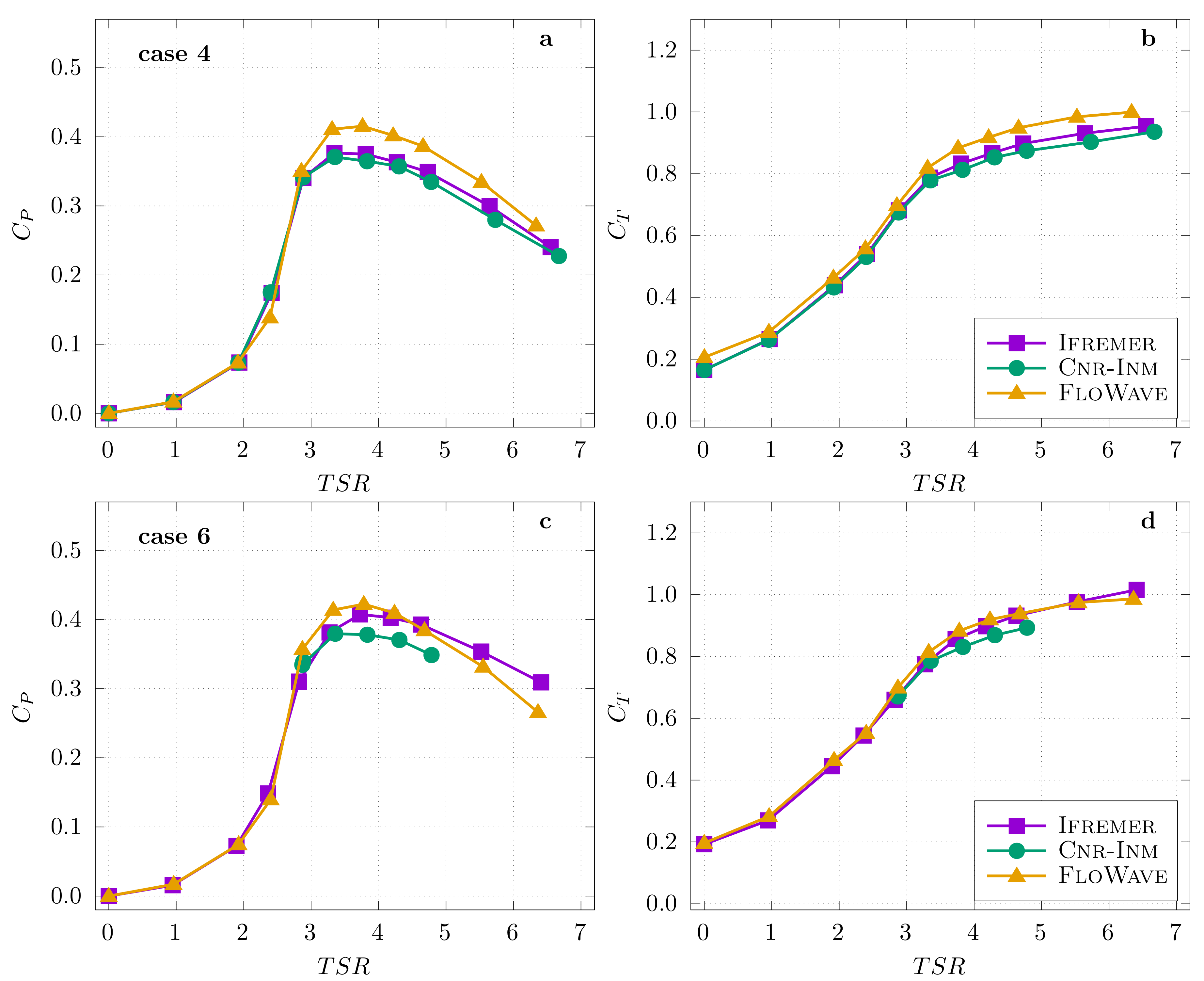
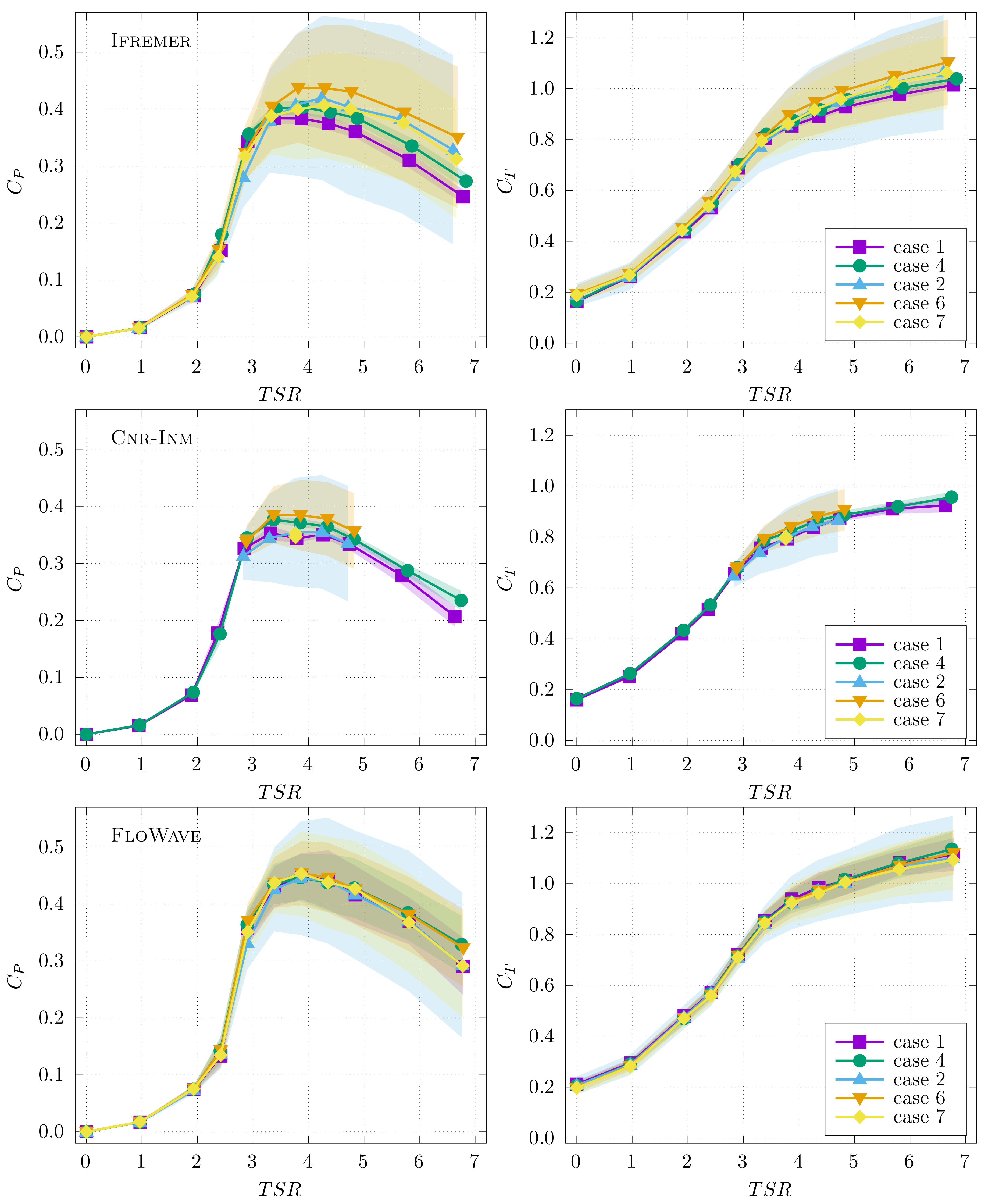
Appendix A. Turbine Performance Comparison within an Individual Test Site

Figure A1 displays the same turbine performance coefficients than those presented on Figure 14 and Figure 15. They are however shown within an individual test site. From these curves, results obtained at IFREMER show the smallest values for current-only cases 1 and 4. On the contrary, the largest ones are observed for the wave and current case 6. Results from CNR-INM show a similar trend but with a smaller gap between the lowest and the largest values: for example, for T S R = 4 , the C P difference is lower than 0.03 at CNR-INM but it is higher than 0.06 at IFREMER. Finally, results from FLOWAVE show very close values for all the cases. The only perceptible difference for the power coefficients is found for the two highest T S R , versus the flow velocity of 0.8 or 1.0 m/s.
Figure A1. Power (left) and thrust (right) coefficients comparison for the same test cases than Figure 14 and Figure 15: 1 current-only at 0.8 m/s, 4 current-only at 1.0 m/s, 2 regular wave with 0.8 m/s, 6 regular wave with 1.0 m/s and 7 irregular wave with 0.8 m/s, versus T S R and displayed within an individual test site
Jmse 08 00463 g0a1

References

  1. Aubrun, S.; Bastankhah, M.; Cal, R.B.; Conan, B.; Hearst, R.J.; Hoek, D.; Hölling, M.; Huang, M.; Hur, C.; Karlsen, B.; et al. Round-robin tests of porous disc models. J. Phys. Conf. Ser. 2019, 1256. [Google Scholar] [CrossRef]
  2. IEC. Marine Energy-Wave, Tidal and Other Water Current Converters-Part 200: Electricity Producing Tidal Energy Converters-Power Performance Assessment; Technical Report; International Electrotechnical Commission: Geneva, Switzerland, 2013. [Google Scholar]
  3. IEC. Marine Energy-Wave, Tidal and Other Water Current Converters-Part 201: Tidal Energy Resource Assessment and Characterization; Technical Report; International Electrotechnical Commission: Geneva, Switzerland, 2015. [Google Scholar]
  4. IEC. Marine Energy-Wave, Tidal and Other Water Current Converters-Part 202: Scale Testing of Tidal Stream Energy Systems; Technical Report; International Electrotechnical Commission: Geneva, Switzerland, 2021. [Google Scholar]
  5. Specialist Committee on Testing of Marine Renewable Devices. Recommended Procedures and Guidelines-Model Tests for Current Turbine. Technical Report. 2017. Available online: https://www.ittc.info/media/8127/75-02-07-038.pdf (accessed on 24 June 2020).
  6. Specialist Committee on Testing of Marine Renewable Devices. Recommended Procedures and Guidelines-Uncertainty Analysis-Example for Horizontal Axis Turbines. Technical Report. 2017. Available online: https://www.ittc.info/media/8141/75-02-07-0315.pdf (accessed on 24 June 2020).
  7. EquiMar. Protocols for the Equitable Assessment of Marine Energy Converters, 1st ed.; Number 213380; The Institute for Energy Systems, The University of Edinburgh: Edinburgh, UK, 2011. [Google Scholar]
  8. Germain, G.; Chapeleau, A.; Gaurier, B.; Macadré, L.M.; Scheijgrond, P. Testing of marine energy technologies against international standards. Where do we stand? In Proceedings of the 12th European Wave and Tidal Energy Conference, Cork, Ireland, 27 August–1 September 2017. [Google Scholar]
  9. Germain, G.; Gaurier, B.; Harrold, M.J.; Ikhennicheu, M.; Scheijgrond, P.; Southall, A.; Trasch, M. Protocols for testing marine current energy converters in controlled conditions.Where are we in 2018? In Proceedings of the 4th Asian Wave and Tidal Energy Conference, Taipei, Taiwan, 9–13 September 2018. [Google Scholar]
  10. Gaurier, B.; Germain, G.; Facq, J.V.; Johnstone, C.; Grant, A.D.; Day, A.H.; Nixon, E.; Di Felice, F.; Costanzo, M. Tidal energy “round Robin” tests comparisons between towing tank and circulating tank results. Int. J. Mar. Energy 2015, 12, 87–109. [Google Scholar] [CrossRef] [Green Version]
  11. Bahaj, A.S.; Molland, A.F.; Chaplin, J.R.; Batten, W.M.J. Power and thrust measurements of marine current turbines under various hydrodynamic flow conditions in a cavitation tunnel and a towing tank. Renew. Energy 2007, 32, 407–426. [Google Scholar] [CrossRef]
  12. Murray, R.E.; Ordonez-Sanchez, S.; Porter, K.E.; Doman, D.A.; Pegg, M.J.; Johnstone, C. Towing Tank and Flume Testing of Passively Adaptive Composite Tidal Turbine Blades. In Proceedings of the 12th European Wave and Tidal Energy Conference, Cork, Ireland, 27 August–1 September 2017. [Google Scholar]
  13. Gaurier, B.; Davies, P.; Deuff, A.; Germain, G. Flume tank characterization of marine current turbine blade behaviour under current and wave loading. Renew. Energy 2013, 59, 1–12. [Google Scholar] [CrossRef] [Green Version]
  14. Galloway, P.W.; Myers, L.E.; Bahaj, A.B.S. Quantifying wave and yaw effects on a scale tidal stream turbine. Renew. Energy 2014, 63, 297–307. [Google Scholar] [CrossRef]
  15. Martinez, R.; Payne, G.S.; Bruce, T. The effects of oblique waves and currents on the loadings and performance of tidal turbines. Ocean Eng. 2018, 164, 55–64. [Google Scholar] [CrossRef]
  16. Ordonez-Sanchez, S.; Allmark, M.; Porter, K.; Ellis, R.; Lloyd, C.; Santic, I.; O’Doherty, T.; Johnstone, C. Analysis of a Horizontal-Axis Tidal Turbine Performance in the Presence of Regular and Irregular Waves Using Two Control Strategies. Energies 2019, 12, 367. [Google Scholar] [CrossRef] [Green Version]
  17. Draycott, S.; Payne, G.; Steynor, J.; Nambiar, A.; Sellar, B.; Venugopal, V. An experimental investigation into non-linear wave loading on horizontal axis tidal turbines. J. Fluids Struct. 2019, 84, 199–217. [Google Scholar] [CrossRef]
  18. McNaughton, J.; Harper, S.; Sinclair, R.; Sellar, B. Measuring and Modelling the Power Curve of a Commercial-Scale Tidal Turbine. In Proceedings of the 11th European Wave and Tidal Energy Conference, Nantes, France, 6–11 September 2015. [Google Scholar]
  19. Durán Medina, O.; Schmitt, F.G.; Calif, R.; Germain, G.; Gaurier, B. Turbulence analysis and multiscale correlations between synchronized flow velocity and marine turbine power production. Renew. Energy 2017, 112, 314–327. [Google Scholar] [CrossRef] [Green Version]
  20. Gaurier, B.; Ikhennicheu, M.; Druault, P.; Germain, G.; Facq, J.V.; Pinon, G. Etude Expérimentale des Effets de Sillage d’un Large Obstacle posé sur le Comportement D’Une Hydrolienne. 2018. Available online: https://archimer.ifremer.fr/doc/00482/59334/62112.pdf (accessed on 24 June 2020).
  21. Gaurier, B.; Germain, G.; Pinon, G. How to correctly measure turbulent upstream flow for marine current turbine performances evaluation? In Advances in Renewable Energies Offshore-Proceedings of the 3rd International Conference on Renewable Energies Offshore, RENEW 2018, Lisbon, Portugal, 8–10 October 2018; Taylor & Francis Group: London, UK, 2019; pp. 23–30. [Google Scholar]
  22. Davies, P.; Germain, G.; Gaurier, B.; Boisseau, A.; Perreux, D. Evaluation of the durability of composite tidal turbine blades. Philos. Trans. R. Soc. A Math. Phys. Eng. Sci. 2013, 371, 20120187. [Google Scholar] [CrossRef] [PubMed]
  23. Suzuki, T.; Mahfuz, H. Fatigue characterization of GFRP and composite sandwich panels under random ocean current loadings. Int. J. Fatigue 2018, 111, 124–133. [Google Scholar] [CrossRef]
  24. Filipot, J.F.; Prevosto, M.; Maisondieu, C.; Le Boulluec, M.; Thomson, J. Wave and turbulence measurements at a tidal energy site. In Proceedings of the 11th Current, Waves and Turbulence Measurement, St. Petersburg, FL, USA, 2–6 March 2015; pp. 1–9. [Google Scholar] [CrossRef] [Green Version]
  25. Draycott, S.; Sutherland, D.; Steynor, J.; Sellar, B.; Venugopal, V. Re-creating waves in large currents for tidal energy applications. Energies 2017, 10. [Google Scholar] [CrossRef] [Green Version]
  26. Gaurier, B.; Germain, G.; Facq, J.V.; Bacchetti, T. Wave and Current Flume Tank of IFREMER at Boulogne-sur-mer. Description of the Facility and Its Equipment; Technical Report; Ifremer: Brest, France, 2018. [Google Scholar] [CrossRef]
  27. Institute of Marine Engineering. Consiglio Nazionale delle Ricerche-Towing Tanks; Institute of Marine Engineering: London, UK, 2019. [Google Scholar]
  28. Sutherland, D.R.; Noble, D.R.; Steynor, J.; Davey, T.; Bruce, T. Characterisation of current and turbulence in the FloWave Ocean Energy Research Facility. Ocean Eng. 2017, 139, 103–115. [Google Scholar] [CrossRef]
  29. Payne, G.S.; Stallard, T.; Martinez, R. Design and manufacture of a bed supported tidal turbine model for blade and shaft load measurement in turbulent flow and waves. Renew. Energy 2017, 107, 312–326. [Google Scholar] [CrossRef]
  30. SixAxes. Société Française, Spécialisée Dans l’étude et la Fabrication de Chaîne de Mesure de Force Depuis plus de 22 Ans; SixAxes: Argenteuil, France, 2017. [Google Scholar]
  31. Goring, D.G.; Nikora, V.I. Despiking acoustic doppler velocimeter data. J. Hydraul. Eng. 2002, 128, 117–126. [Google Scholar] [CrossRef] [Green Version]
  32. Mycek, P.; Gaurier, B.; Germain, G.; Pinon, G.; Rivoalen, E. Experimental study of the turbulence intensity effects on marine current turbines behaviour. Part I: One single turbine. Renew. Energy 2014, 66, 729–746. [Google Scholar] [CrossRef] [Green Version]
  33. Blackmore, T.; Myers, L.E.; Bahaj, A.S. Effects of turbulence on tidal turbines: Implications to performance, blade loads, and condition monitoring. Int. J. Mar. Energy 2016, 14, 1–26. [Google Scholar] [CrossRef] [Green Version]
  34. Huang, N.E.; Shen, Z.; Long, S.R.; Wu, M.C.; Shih, H.H.; Zheng, Q.; Yen, N.C.; Tung, C.C.; Liu, H.H. The empirical mode decomposition and the Hilbert spectrum for nonlinear and non-stationary time series analysis. R. Soc. London. Ser. A Math. Phys. Eng. Sci. 1998, 454, 903–995. [Google Scholar] [CrossRef]
  35. Brevik, I.; Bjørn, A. Flume experiment on waves and currents. I. Rippled bed. Coast. Eng. 1979, 3, 149–177. [Google Scholar] [CrossRef]
  36. Klopman, G. Vertical structure of the flow due to wave and currents-Laser-Doppler flow measurements for waves following or opposing a current. In WL Report H840-30, Part II, for Rijkswaterstaat; Technical Report; Deltares (WL): Delft, The Netherlands, 1994. [Google Scholar]
  37. Guo, X.; Yang, J.; Gao, Z.; Moan, T.; Lu, H. The surface wave effects on the performance and the loading of a tidal turbine. Ocean Eng. 2018, 156, 120–134. [Google Scholar] [CrossRef]
  38. Draycott, S.; Steynor, J.; Davey, T.; Ingram, D.M. Isolating incident and reflected wave spectra in the presence of current. Coast. Eng. J. 2018, 60, 39–50. [Google Scholar] [CrossRef]
  39. Gaurier, B.; Ordonez-Sanchez, S.; Germain, G.; Facq, J.V.; Johnstone, C.; Salvatore, F.; Santic, I. MaRINET2 Tidal “Round Robin” Dataset: Comparisons Between Towing and Circulating Tanks Test Results for a Tidal Energy Converter Submitted to Wave and Current Interactions. SEANOE: Brest, France, 2018. [Google Scholar] [CrossRef]
Figure 1. Side views (top) and top view (bottom) of the flume tank of IFREMER at Boulogne-sur-mer, France.
Jmse 08 00463 g001
Figure 2. Schematic of the towing tank of CNR-INM at Rome, Italy.
Jmse 08 00463 g002
Figure 3. Schematic of the FLOWAVE circular combined wave and current test tank at Edinburgh, UK.
Jmse 08 00463 g003
Figure 4. The 3-bladed instrumented turbine in the wave and current flume tank of IFREMER (top left-hand side), in the towing tank of CNR-INM (top right-hand side) and in the FLOWAVE circular wave and current tank (bottom).
Jmse 08 00463 g004
Figure 5. Schematic of the blade roots and the waterproof torque Q and thrust T transducer.
Jmse 08 00463 g005
Figure 6. Schematic top-view of the test set-up used in the tanks. ADV is used in every tank but the seeding mast is required at CNR-INM only. The wave gauges 1 to 3 are used at IFREMER and FLOWAVE. Wave gauges 3 to 6 at CNR-INM. Dimensions are given in mm and the presented tank width represents the IFREMER size.
Jmse 08 00463 g006
Figure 7. Front view of the ADV measurement points depicted by red circles inside the turbine swept area and their coordinates expressed in mm.
Jmse 08 00463 g007
Figure 8. Vertical profiles of the average and standard-deviation of the stream-wise component of the velocity at the turbine location. Numbers 1 to 7 stand for the 7 different generated test cases (see Table 3).
Jmse 08 00463 g008
Figure 9. Disc-integrated velocity average: the Acoustic Doppler Velocimeter (ADV) measurements profile (case 6 at IFREMER flume tank) is spline fitted and extended in the transverse y direction (coloured plot). The spatial average is then processed on the turbine swept area (dashed black line). In this example, U = 1.047 m/s.
Jmse 08 00463 g009
Figure 10. Average and standard-deviation of the transverse v and vertical w span-wise components of the velocity measured with ADV at z = 0 ( P 0 , P 3 and P 4 ) versus case numbers.
Jmse 08 00463 g010
Figure 11. Turbulence intensity I 3 D processed from the velocity measured with ADV at z = 0 ( P 0 , P 3 and P 4 ) versus case numbers. For the wave and current tests, the wave frequency component has been filtered and removed from the velocity measurements.
Jmse 08 00463 g011
Figure 12. Vertical profiles of the average and standard-deviation of the amplitude of the Hilbert transform of the stream-wise component of the velocity at the turbine location. Numbers 2 to 7 stand for the different generated test cases (see Table 3).
Jmse 08 00463 g012
Figure 13. Average and standard-deviation of the amplitude of the Hilbert transform of the surface elevation η , at the turbine location, versus the case number (see Table 3).
Jmse 08 00463 g013
Figure 14. Power (a,c) and thrust (b,d) coefficients comparison for current-only cases: 1 at 0.8 m/s (a,b) and 4 at 1.0 m/s (c,d), versus T S R .
Jmse 08 00463 g014
Figure 15. Power (a,c,e) and thrust (b,d,f) coefficients comparison for wave and current cases: 2 regular wave with 0.8 m/s (a,b), 6 regular wave with 1.0 m/s (c,d) and 7 irregular wave with 0.8 m/s (e,f), versus T S R (see Table 3 for cases details).
Jmse 08 00463 g015
Figure 16. Blockage correction factor ( U T / U F ) 3 versus T S R to be applied to the power coefficient, according to the method presented by Bahaj et al. [11]. These coefficients are processed from case 4 (current-only at 1.0 m/s).
Jmse 08 00463 g016
Figure 17. Power (a,c) and thrust (b,d) coefficients comparison accounting for blockage correction: Case 4 with current-only at 1.0 m/s (a,b), case 6 with regular wave and current of 1.0 m/s (c,d), versus T S R .
Jmse 08 00463 g017
Figure 18. Power (a) and thrust (b) coefficients comparison for current-only case 4 at 1.0 m/s without wavemaker and with the parked wavemaker at IFREMER, versus T S R , showing the turbulence effects on the turbine performance.
Jmse 08 00463 g018
Figure 19. Power production of the turbine P versus the water level η measured by the wave probe 3 (cf. Figure 6), for the wave and current case 2 at T S R = 4 . Green points stand for the raw data and violet curve is the wave phase average of the power versus the wave phase average of the surface elevation.
Jmse 08 00463 g019
Figure 20. Power production of the turbine P versus the stream-wise fluctuation of the velocity u measured by the ADV on the side of the turbine (cf. Figure 6), for the wave and current case 2 at T S R = 4 . Green points stand for the raw data, violet curve is the wave phase average of the power versus the wave phase average of the fluctuating velocity and dashed line stands for its best linear fit.
Jmse 08 00463 g020
Table 1. Testing facilities main characteristics. Note that the maximum velocity is limited in the flume tanks when including waves. The diameter of the FLOWAVE tank is 25 m according to schematic Figure 3, but an equivalent usable length of 15 m is considered in the following sections.
Laboratory NameIFREMERCNR-INMFLOWAVE
Type of tankflumetowingflume
Length [m]1822015
Width × Depth [m]4 × 29 × 3.515 × 2
Blockage ratio [%]5.11.31.4
Speed range [m/s]0.1 to 2.20.1 to 100.1 to 1.6
Turbulence int. [%]1.5 to 15NA5 to 11
Wave freq. [Hz]0.5 to 20.4 to 1.250.2 to 1.2
Wave max. amp. [mm]150450450
Table 2. Transducer measuring range.
Torque and Thrust Transducer
Thrust500 N
Torque50 N·m
Table 3. Summary of the test matrix. The wave parameters are the required ones, that is, in every tank these characteristics have to be adjusted to account for the flow velocity (amplitude) or the carriage motion (frequency).
CaseTypeFlow SpeedWaveWave
[m/s]freq. [Hz]ampl. [mm]
1current0.8--
2regular0.80.675
3regular0.80.535
4current1.0--
5regular1.00.775
6regular1.00.655
7irregular0.8 T P = 1.67  s H S = 100  mm
Table 4. U expressed in m/s and processed with the disc-integrated method from ADV measurements carried out without the turbine.
Case #IFREMERCNR-INMFLOWAVE
10.8260.8430.825
20.8480.8480.827
30.846NA0.822
41.0241.0371.036
51.0561.036NA
61.047NA1.031
70.840NA0.826
Table 5. Average and standard-deviation of the row power and thrust measured on the turbine for current-only cases (1 and 4) and for combined wave and current cases (2, 6 and 7). For each case and each tank, T S R is chosen to correspond to the highest power value, that is,  T S R 4 . Numbers highlighted in colour correspond to the highest (red) or lowest (blue) parameter values, for each tested case.
Case #14267
P ¯ [W]IFREMER44.589.256.4109.252.0
CNR-INM43.886.945.789.545.4
FLOWAVE52.9104.053.5104.553.7
σ ( P ) [W]IFREMER1.22.919.424.011.8
CNR-INM1.51.212.811.65.5
FLOWAVE4.89.612.013.08.8
T ¯ [N]IFREMER112.9188.7139.0206.6135.3
CNR-INM111.0174.5125.6176.2119.5
FLOWAVE132.5206.1131.5204.2130.8
σ ( T ) [N]IFREMER1.53.225.324.416.6
CNR-INM0.81.817.911.57.7
FLOWAVE6.09.815.013.310.9

