Validation and Application of a New Software Tool Implementing the PISA Design Methodology

Abstract

The PISA (Pile Soil Analysis) research project has resulted in a new methodology for the design of offshore wind turbine monopile foundations. A new software tool called PLAXIS Monopile Designer (MoDeTo) has been developed that automates the PISA design methodology. It facilitates the calibration of the so-called soil reaction curves by automated three-dimensional finite element calculations and it allows for a quick design of monopiles using the calibrated soil reaction curves in a one-dimensional finite element model based on Timoshenko beam theory. The monopile design approach has been validated for sand- and clay-type soils which are common in North Sea soil deposits. The paper presents a validation exercise based on the PISA research project proposal of a rule-based parametric model—General Dunkirk Sand Model (GDSM)—for Dunkirk sand as well as an application of the tool for a project involving an offshore wind turbine on a monopile foundation in sandy layered soil in which the PISA design is compared to the conventional API design. The paper concludes with a discussion of the results and the differences between the various methods.

1. Introduction

In the last decade, offshore wind has proven to become a viable option in the transition from fossil to renewable energy sources. Given the relatively shallow depth of the southern part of the North Sea, monopiles are the most favorable and cost-effective type of wind turbine foundations, and the further evolution beyond XL monopiles will extend their applicability to larger wind turbines and potentially deeper water depths in the future.

The PISA (Pile Soil Analysis) joint industry research project [1,2,3] has led to an innovative design methodology for monopiles. In contrast to conventional design methods, it takes account of the positive effects of large diameter piles when subjected to bending moment and lateral loading at the top. Within the PISA method distinction is made between numerical-based design (NBD) and rule-based design (RBD). In the former, three-dimensional (3D) finite element calculations are performed to calibrate soil reactions within a given design space or calibration space (range of lengths, diameters, and other design parameters). The calibrated soil reactions, representing particular soil types or ground profiles, are then used alongside a one-dimensional (1D) Timoshenko beam model with Winkler spring supports, to perform site-specific design optimizations. Alternatively, the PISA method allows for the RBD, in which pre-calibrated soil reactions for different soil types are used; the latter is mostly used in concept design studies.

In collaboration with the University of Oxford, the PISA design methodology was implemented in a validated software tool called PLAXIS Monopile Designer or Monopile Design Tool (MoDeTo) [4,5,6]. This tool automates the creation and calculation of 3D finite element models and the process of calibrating soil reaction curves, and it facilitates the quick design optimization by means of a 1D finite element beam model using the calibrated soil reaction curves.

Meanwhile, the PISA research group has worked on a dedicated soil model for Dunkirk sand, the General Dunkirk Sand Model (GDSM) [7]. This 1D model, consisting of a set of rule-based parameterized soil reaction curves, validated for various relative densities, is supposed to form a good representation of sandy soil layers in the southern part of the North-Sea. The GDSM is used in the first part of this paper to validate the monopile designer for sandy soils. The second part of this paper describes a practical application involving a wind turbine on a monopile foundation in a sandy layered seabed. The paper ends with a discussion of the results and conclusions.

2. Method

According to the PISA design methodology, soil reaction curves are defined as four-parameter conic functions in which the parameters are depth-dependent. There are four types of soil reactions: (1) lateral stress along the shaft, (2) bending moment along the shaft as a result of opposite shear stress in the front and rear side of the pile, (3) shear stress at the base, and (4) bending moment as a result of normal stress distribution at the base. Hence a total of 16 depth-dependent parameters are defined in terms of depth variation functions (dvf’s). In the NBD, the determination and calibration of the dvf’s is based on a series of 3D finite element calculations and the requirement that the area between the load-displacement curve from the 3D finite element models and the curve from the corresponding 1D Timoshenko beam model with soil reactions, is minimized using a two-step optimization procedure (first-stage calibration + correction). The optimization is based on normalized soil reaction curves. For details on the optimization method and corresponding accuracy metric η, reference is made to Byrne et al. 2019 [8]. The finite element models shall cover a range of monopile dimensions with variations in height above mudline where the load is applied (h), embedment depth (L), outer diameter (D_out), and wall thickness (t). This so-called calibration space or design space is used to provide some flexibility in optimizing the final design while ensuring the validity of the calibrated soil reactions, as long as the final design is within this space.

3. Validation of Monopile Designer for Dunkirk Sand

In the first part of this contribution we consider the validation of the monopile designer based on the Sand modelling framework as described in Burd et al. [7], for which sandy soils with a relative density (D_r) in the range 45% ≤ D_r ≤ 90% were considered. Burd et al. describe the General Dunkirk Sand Model (GDSM) as a collection of soil reactions in which the coefficients in the dvf’s have been expressed in terms of D_r. The GDSM has been validated for monopiles with an L/D ratio in the range 2–6 and a h/D ratio in the range 5–15.

For our validation of the monopile designer we consider Dunkirk sand with a relative density of 75%. As a reference, we use the soil reactions based on the GDSM for D_r = 75%, backed by the original 3D finite element calculations used for the calibration/validation of the GDSM with the Critical State constitutive model for sand by Taborda et al. [9]. The soil profile as defined in the monopile designer is listed in

Table 1. Soil profile, as defined in the monopile designer, representing Dunkirk sand with D_r = 75%.

Top (m)	Bottom (m)	γ′ (kN/m3)	G0,mid (MN/m2)	φ′ (°)	Ψ (°)	K0 (-)
0	−90	10.09	205.3	39	9	0.37

. For the Numerical Based Design (NBD), this soil profile was translated into a single soil layer when generating the PLAXIS 3D finite element models, using the Hardening Soil small-strain (HSsmall) model by Benz [10] with drained (effective) parameters as listed in

Table 2. Parameters of the Hardening Soil small-strain (HSsmall) model, representing Dunkirk sand with D_r = 75%.

Parameter	Symbol	Value	Unit
Effective unit weight	γ′	10.09	kN/m3
Reference secant stiffness in triaxial compression	E50ref	45,000	kN/m2
Reference tangent stiffness in primary oedometric loading	Eoedref	45,000	kN/m2
Reference triaxial unloading/reloading stiffness	Eurref	135,000	kN/m2
Stress-dependency of stiffness	m	0.5	-
Effective cohesion	c′	0.1	kN/m2
Effective friction angle	φ′	39	°
Dilatancy angle	Ψ	9.0	°
Strain at which G has reduced to 70%	γ0.7	0.000125	-
Reference small-strain shear modulus	G0ref	194,000	kN/m2
Reference stress	pref	100	kN/m2
Unloading/reloading Poisson’s ratio	νur	0.2	-
K0 stress ratio in normally consolidated condition	K0nc	0.3707	-
Friction ratio	Rf	0.906	-
Tensile strength	σt	0.0	kN/m2

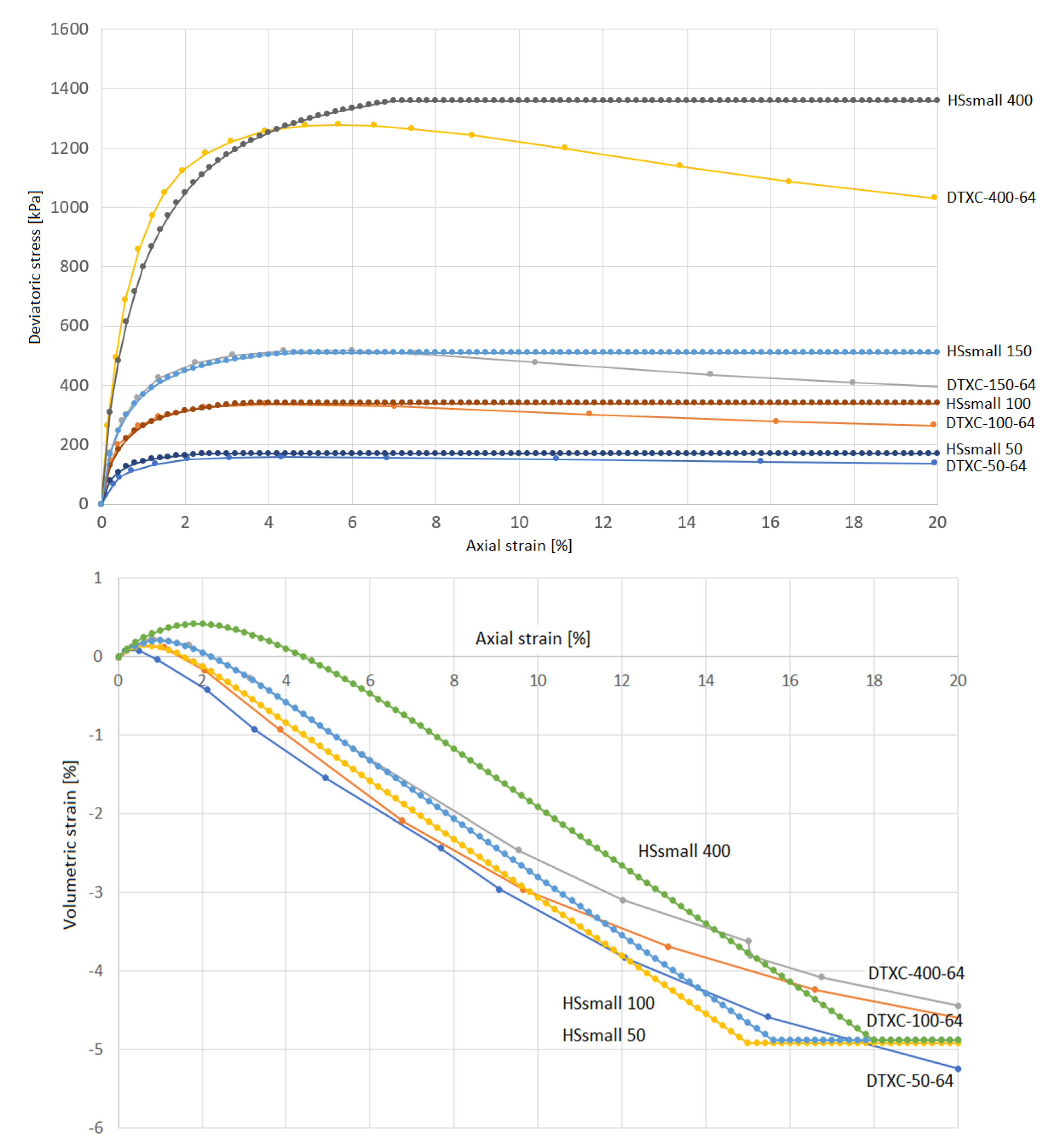
. Parameter values are mostly based on correlations by Brinkgreve et al. [11], considering D_r = 75%. The HSsmall parameter set was tested under drained triaxial compression test conditions at initial isotropic stresses of 50, 100, 150, and 400 kN/m², and the stress–strain behavior was compared with triaxial test data on Dunkirk sand with an initial void ratio of e₀ ≈ 0.64 (D_r ≈ 75%) from the PISA project, digitized from [9]. A dilatancy cut-off was imposed at a maximum void ratio of 0.72, equivalent to a volumetric strain (expansion) of nearly 5%, to account for Critical State. Results of the triaxial test simulations (HSsmall ###) in comparison with digitized lab test data (DTXC-###-64) are shown in Figure 1, where ### indicates the corresponding initial isotropic stress in kN/m². Although HSsmall does not capture the softening behavior, the overall stress and strain response is quite accurate for these test conditions.

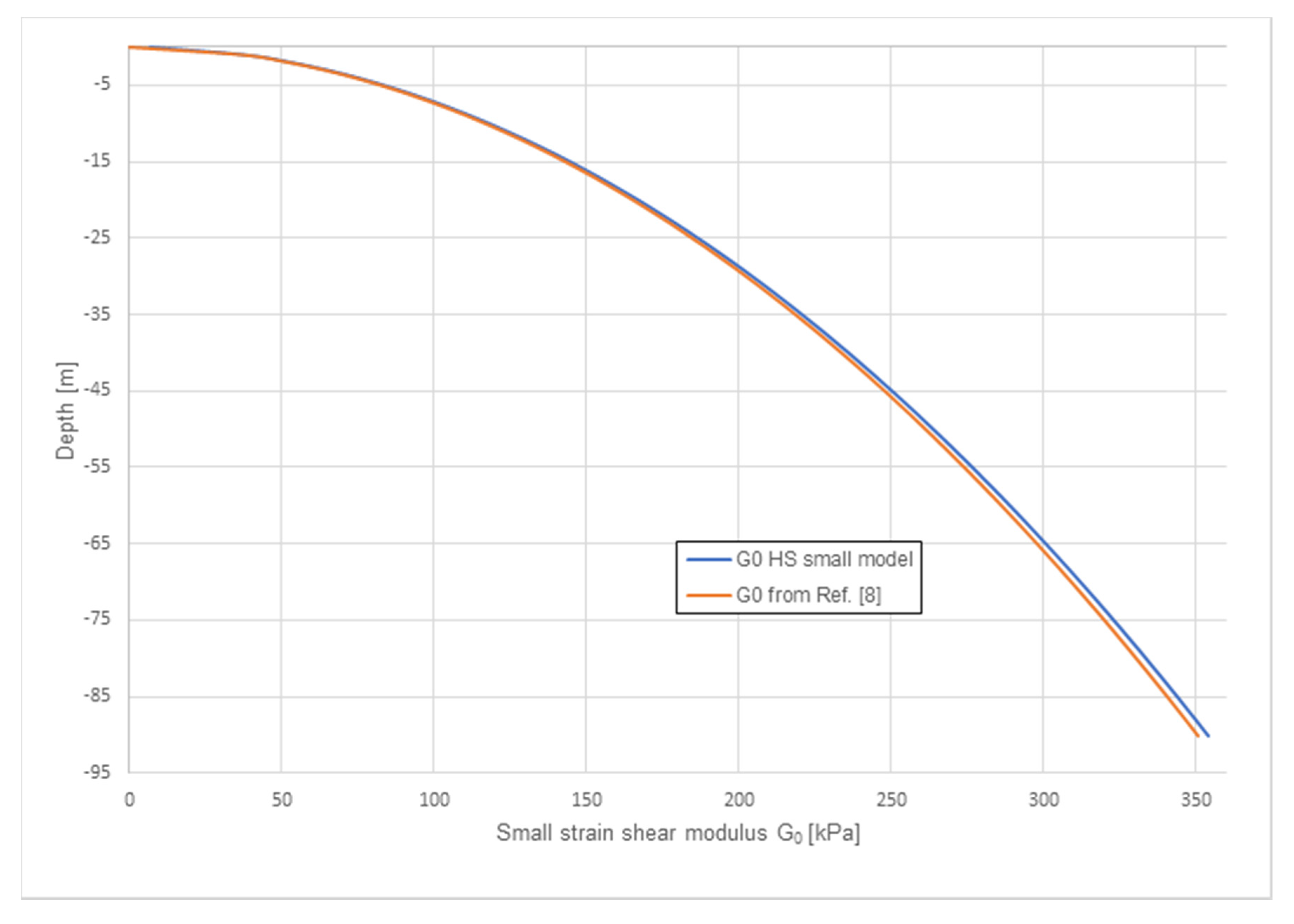
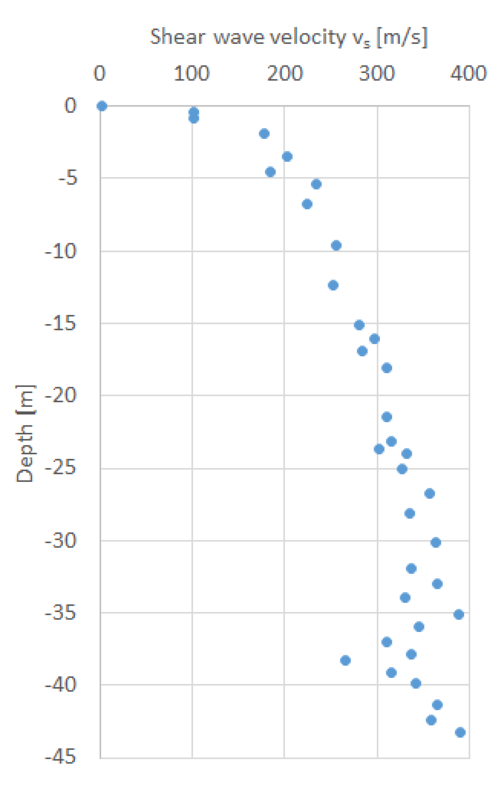
An important parameter is the small-strain shear modulus G₀. In the HSsmall model, this parameter is stress-dependent and hence depth-dependent. With a reference value G₀^ref = 194,000 kN/m² for a reference confining pressure of 100 kN/m² this will give the G₀-profile as depicted in Figure 2. The G₀-profile is plotted over digitized data from [9]. It can be concluded that the modelled G₀-profiles are quite similar.

To calibrate the soil reaction curves, a calibration space with nine models was defined, with design parameter combinations as listed in

Table 3. Calibration space for validation case.

Model	h (m)	L (m)	Dout (m)	h/D (-)	L/D (-)	t (m)	vmax (m)
1	50	20	10.0	5.0	2.0	0.091	9.9
2	75	20	10.0	7.5	2.0	0.091	14.0
3	100	40	10.0	10.0	4.0	0.091	7.8
4	75	40	10.0	7.5	4.0	0.091	10.8
5	25	10	5.0	5.0	2.0	0.045	5.1
6	25	20	5.0	5.0	4.0	0.045	4.3
7	50	20	5.0	10.0	4.0	0.045	6.1
8	75	15	7.5	10.0	2.0	0.068	7.5
9	37.5	30	7.5	5.0	4.0	0.068	6.0

. This calibration space was chosen after a preliminary analysis in which the h/D-range and L/D-range were investigated. It is narrower than what was considered for the GDSM development. Our observation is that using a narrow h/D and L/D range in the calibration space produces more accurate soil reaction curves. In practice, designers generally have a good feel for appropriate monopile dimensions, so ranges can be narrow.

To assure sufficient data, far into the nonlinear range of soil reactions, a lateral prescribed displacement v_max is applied at the top of the pile (z = h) such that at mudline level (z = 0) a lateral displacement around 0.2 times the pile diameter is obtained in the last calculation phase.

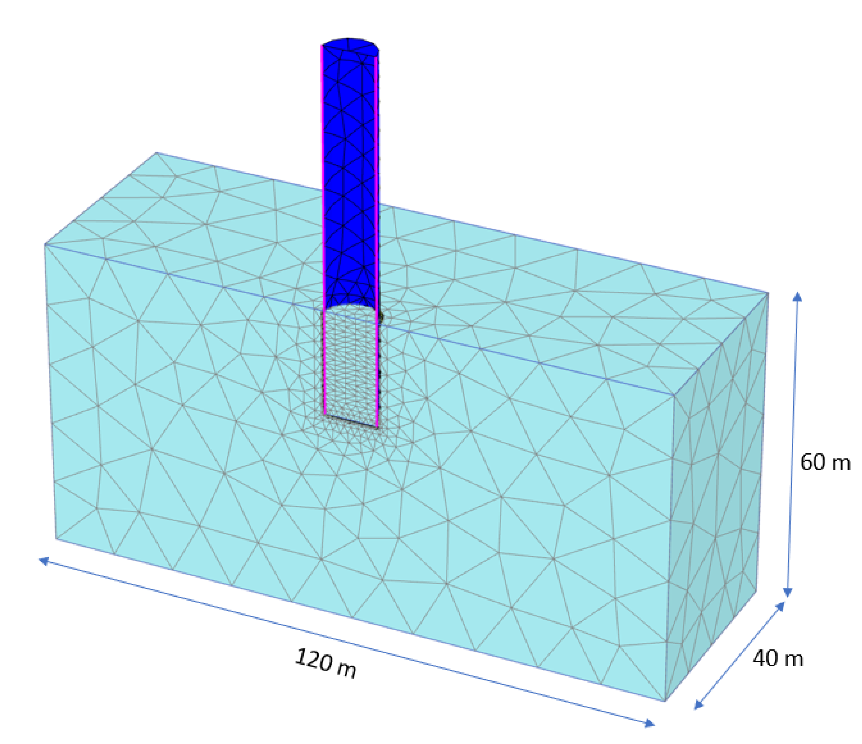
The finite element models generated by the monopile designer are optimized in terms of element mesh and calculation steps such that an accurate solution is obtained within an acceptable calculation time. For details on the choices made in the automated model generation, the reference is made to the PLAXIS MoDeTo manual [4]. Only one symmetric half of the 3D geometry is modelled. The mesh consists of quadratic 10-node tetrahedral soil elements and six-node MITC6 shell elements for the steel pile wall. Steel properties are defined by linear elastic behavior with Young’s modulus E = 200·10⁶ kN/m² and Poisson’s ratio ν = 0.3. Between the pile wall and the soil and at the pile base, 12-node interface elements are used to model soil-structure interaction and to ‘collect’ the soil reactions. In absence of softening and Critical State behavior, the wall friction angle in the interface elements is assumed 29° and the dilatancy angle 0°. One of the used finite element models is shown in Figure 3.

Each model calculation consists of four calculation phases; each calculation is performed according to small-deformation theory and in all calculations the soil behavior is assumed drained: (Phase 1) setting up the initial stress state; (Phase 2) activating the monopile; (Phase 3) applying prescribed displacement for small displacement solution (0.001·v_max); (Phase 4) applying prescribed displacement for large displacement solution (v_max). It is the idea that Phase 3 provides accurate data to calibrate the small-strain response, which is needed for any Fatigue Limit State (FLS) design criterion, while Phase 4 provides data to calibrate the large strain response and bearing capacity, which is needed for any Ultimate Limit State (ULS) design criterion.

4. Validation Results

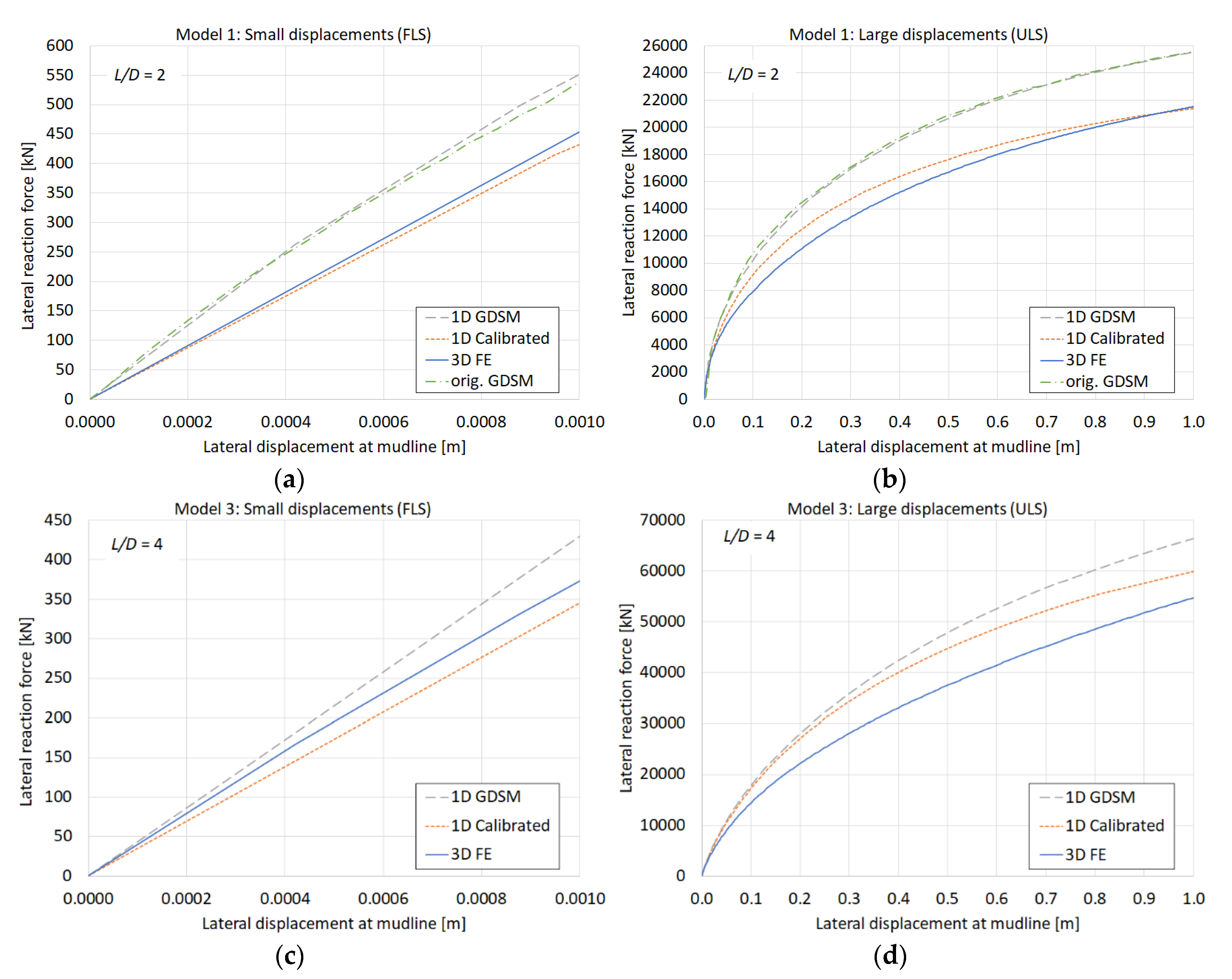
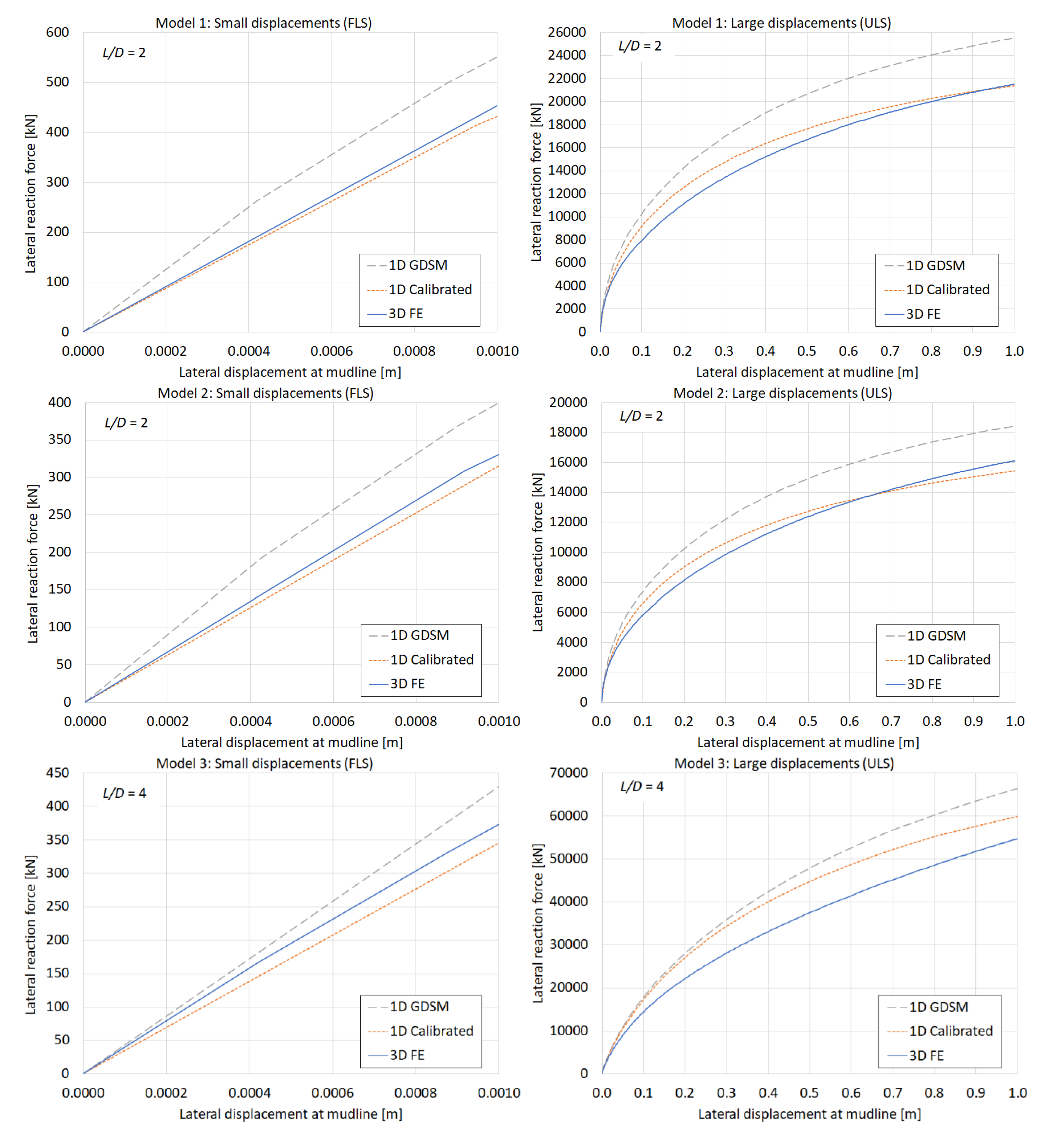
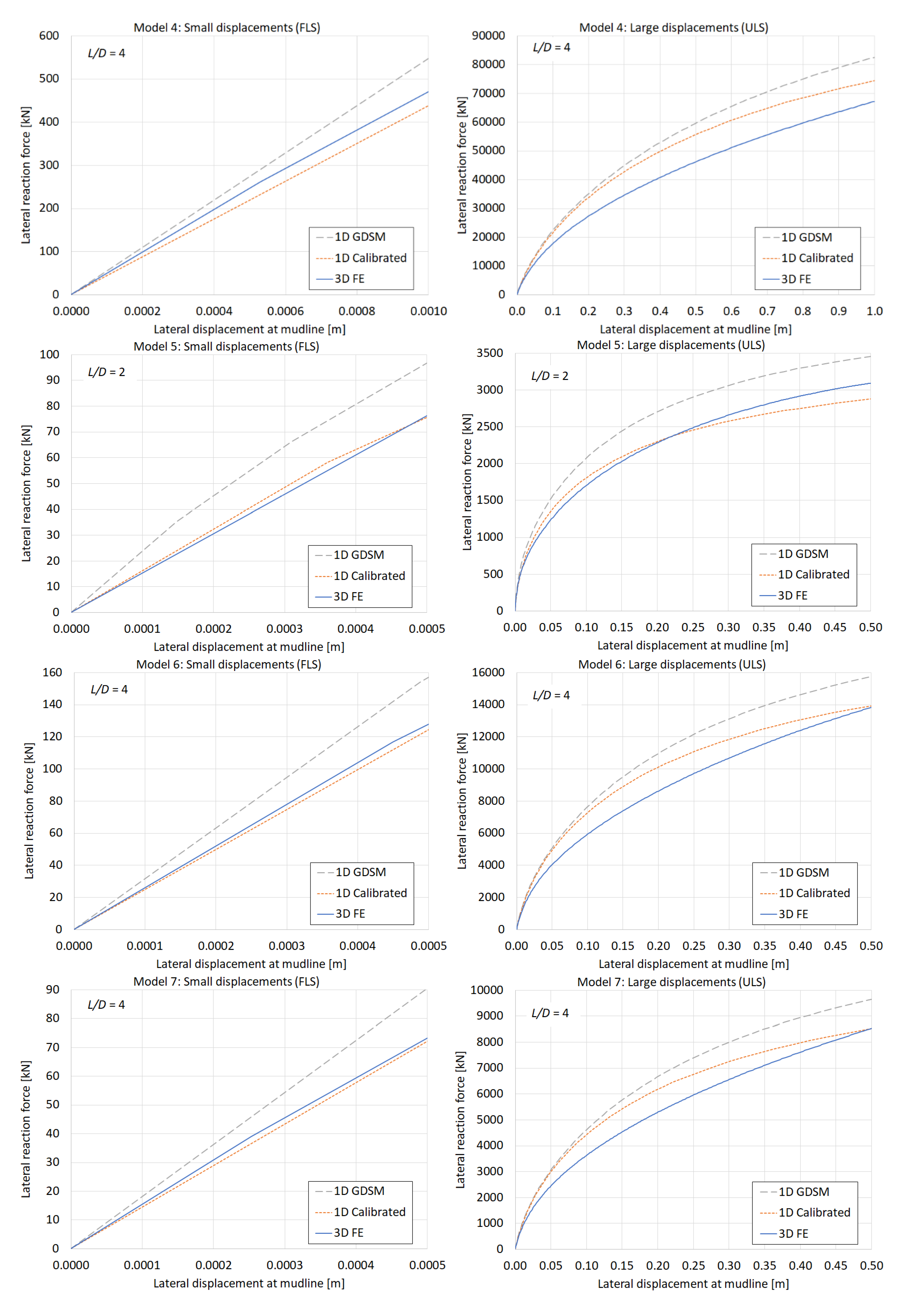
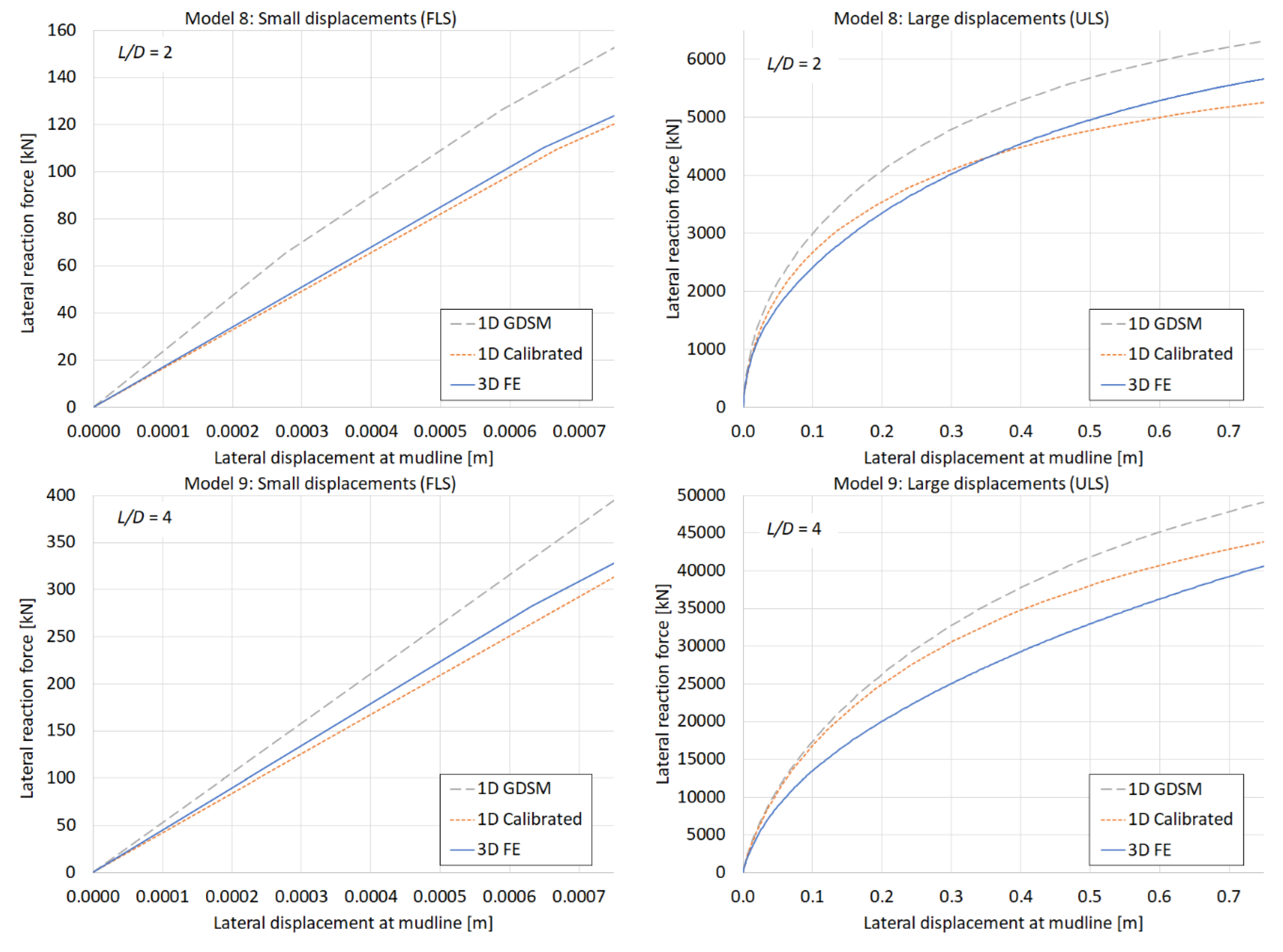
Figure 4 shows load-displacement curves (lateral reaction force due to prescribed displacement versus lateral displacement at mudline level to a maximum of 0.1·D) from two of the Models 1–9 (Model 1 and 3); a complete overview of results is shown in Appendix A, with an indication of the accuracy metric η for each 3D model and the corresponding 1D model; both for small (FLS) and large (ULS) displacements. Each graph shows (1) the curves from the 3D finite element calculations (3D FE), (2) the 1D calculations from the monopile designer with the calibrated soil reactions based on the 3D finite element models (1D Calibrated), and (3) the 1D calculations from the monopile designer with soil reactions according to the GDSM as a reference solution (1D GDSM). Moreover, the results for Model 1 also include a comparison with digitized data from the original GDSM calculation for the same case (Model 1 ≅ C1) by the PISA research team [7], which validates the GDSM implementation in the monopile designer.

We can discover some trends in the curves.

• Overall, the small displacement solutions of the calibrated 1D models (1D Calibrated) are similar as the corresponding 3D finite element solutions (3D FE), whereas they are conservative compared to the GDSM solutions (1D GDSM).
• For large displacements, the 1D Calibrated solutions are more ‘curved’ than the corresponding 3D FE solutions. In most cases, this results in a higher load in the mid displacement range, but also a ‘bearing capacity’ at maximum displacement that is closer to the corresponding 3D FE solution (some are even lower).
• For large displacements, the 3D FE solutions overall show a lower stiffness and bearing capacity compared to the GDSM solutions, but the corresponding 1D Calibrated solutions are generally closer to GDSM solutions.
• Following points 2 and 3 (for large displacements), distinction can be made between the lower and higher L/D ratios: for the higher L/D ratios (L/D = 4; Models 3, 4, 6, 7, and 9), the 1D Calibrated solutions tend to be stiffer than the 3D FE solutions and show a better correspondence to the GDSM solutions than for the lower L/D ratios (L/D = 2; Models 1, 2, 5, and 8). A further nuance for the low L/D ratios can be seen in that the 1D Calibrated solutions tend to be better (at least in terms of bearing capacity) for larger diameter piles (Models 1 and 2).
• No clear trend can be observed with respect to the h/D ratio.

A further analysis revealed that the calibration of soil reaction curves, based on a simple two-step parameterization (first-stage calibration + correction), may not be accurate enough and may require a more refined parameter optimization. To improve this, the so-called second-stage optimization might be implemented in the calibration procedure [7,8]. This improvement could reduce the curvature of the 1D Calibrated curves, such that they better match the 3D FE curves, although they will be generally on the conservative side compared to the GDSM solutions (just like the 3D FE solutions), at least for normally consolidated stress states.

5. Application Case: 11 MW Wind Turbine in the North Sea

In this section we describe a realistic case involving a 11 MW wind turbine at a particular site in the North Sea, dominated by sandy layered soil, for which the ground conditions apply as listed in

Table 4. Soil strata and corresponding relative density (D_R) and over-consolidation ratio (OCR) at the project site.

Top (m)	Bottom (m)	DR (%)	OCR (-)
0	−2	82	1.0
−2	−3.9	65	10.0
−3.9	−6.5	62	10.0
−6.5	−9.6	61	10.0
−9.6	−13.2	59	8.0
−13.2	−17.3	64	6.1
−17.3	−20.7	65	5.1
−20.7	−23.8	57	4.4
−23.8	−25.8	68	4.1
−25.8	−30.0	73	3.7
−30.0	−31.0	72	3.5
−31.0	−32.5	61	3.3
−32.5	−60.0	70	3.2

and shown in Figure 5.

The ground conditions in Table 4 and Figure 5 were translated into distinct soil layers with varying properties, as listed in

Table 5. Soil data of the application case.

Top (m)	Bottom (m)	γ′ (kN/m3)	G0 (MN/m2)	φ′ (°)	Ψ (°)	K0 (-)
0	−2	7.9	51.89	41	11	0.3
−2	−3.9	9.1	50.08	39	9	1.6
−3.9	−6.5	9.6	52.44	39	9	1.6
−6.5	−9.6	9.9	66.19	39	9	1.6
−9.6	−13.2	10.0	87.50	38	8	1.4
−13.2	−17.3	10.2	122.01	39	9	1.2
−17.3	−20.7	10.4	150.85	39	9	1.0
−20.7	−23.8	10.1	161.33	38	8	1.0
−23.8	−25.8	10.6	185.13	40	10	0.9
−25.8	−30.0	10.9	196.30	40	10	0.8
−30.0	−31.0	11.0	212.42	40	10	0.8
−31.0	−32.5	10.6	196.46	39	9	0.8
−32.5	−60.0	11.0	299.31	40	10	0.8

.

To calibrate the soil reactions for this case, a calibration space with eight models was defined with design parameter combinations as listed in

Table 6. Calibration space for the application case.

Model	h (m)	L (m)	Dout (m)	t (m)	vmax, z = h (m)
1	30	24	6.0	0.08	4.5
2	72	24	6.0	0.08	9.0
3	30	12	6.0	0.08	6.0
4	72	12	6.0	0.08	13.0
5	63	36	9.0	0.08	8.5
6	90	36	9.0	0.08	12.0
7	63	18	9.0	0.08	12.0
8	90	18	9.0	0.08	16.5

. Once the parameter combinations are defined, the whole process to Generate the models, to Calculate the models, and to Parameterize the soil reactions, is fully automated, but it takes several hours to complete this step. An example of a calculated finite element model is shown in Figure 6. The results of the calibration can be visualized in terms of load-displacement curves, pile deflection curves, soil reaction curves (the four components) for all individual models as well as the calibrated dvf’s of the parameters of the soil reaction curves (not presented herein).

6. Design Optimization

The calibrated soil reactions were used in the 1D calculation to design the monopile. The loading conditions (except the vertical component, which is absent here), are in line with Panagoulias et al. [12]; however, note that the site conditions are different here in the sense that the soil is less competent (on average, lower G₀, smaller φ′, smaller OCR). The loading involves a static lateral load H = 15 MN acting at a height h = 35 m, resulting in a bending moment M = 525 MNm at mudline level.

In principle, the following design criteria are applicable:

• Serviceability Limit State (SLS) criterion: under a lateral load H acting at height h, the average rotation at mudline must be less than 0.25°.
• Ultimate Limit State (ULS) criterion: considering a global safety factor of 1.5 according to the Working Stress Design approach, the working load shall be increased by this factor to obtain the design load, and the resulting lateral displacement at mudline must be less than 0.1 times the monopile diameter.

For the design process an initial embedment depth L = 30 m was assumed, with the idea to optimize the design parameter L, while the height above mudline h, the diameter D and the wall thickness t were preselected and assumed constant (h = 35 m, D = 8.0 m, and t = 0.08 m).

The design was optimized by subsequently changing the embedment depth L (in steps of 1 m) until both SLS and ULS design criteria were just satisfied. This process is rather quick, since it requires only a few seconds to run the 1D analysis and to inspect the results for a given combination of design parameters against the design criteria. In this way, an optimized embedment depth L = 38 m (L/D = 4.75) was found, based on the SLS design criterion, whereas the ULS criterion lead to an embedment depth of L = 21 m, which is not decisive here. Based on the 1D design model with L = 38 m, a 3D design verification finite element model was generated and calculated, which proved that the results are indeed within the design criteria. In fact, using more 3D FE calculations, the embedment depth could be further reduced to L = 33 m to just meet the SLS design criterion.

Two issues shall be noticed here:

• There is a significant difference between the embedment depth resulting from the SLS design criterion and the ULS design criterion.
• The L/D ratio (4.75) exceeds the range that was considered in the calibration space [2,3,4], so the 1D results may be unreliable.

In addition to the PISA design method, the design was also performed according to the ‘p-y approach’ [13] to enable a comparison with the conventional API design method. This method is also available in the monopile designer. It resulted in an embedment depth of L = 27 m based on the SLS criterion. However, the reliability of the API design is also debated here, since the pile’s load-deflection behavior is much stiffer than what is obtained from the 3D FE calculation, while the latter is supposed to be the better representation of the real situation. More details on this issue will be provided in Section 7.

7. Discussion of Results

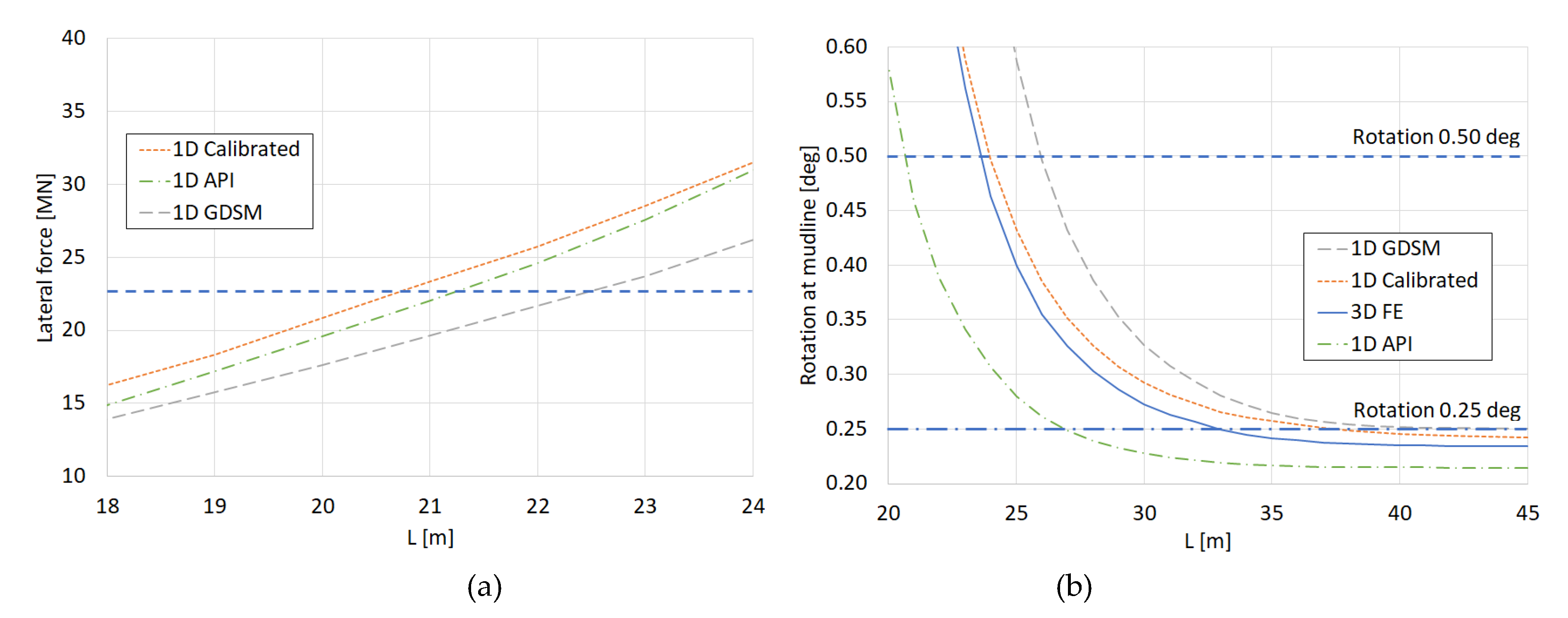
In addition to the design optimization, more insight was obtained in the influence of the embedment depth L by performing various calculations and comparing the results from different design methods in view of the SLS and ULS design criteria. Figure 7a shows the results for the ULS conditions (bearing capacity defined as the design load giving a displacement of 0.1 D at mudline; design capacity is 22.5 MN) and Figure 7b shows the results for the SLS conditions (rotation θ at mudline for the working load; design threshold is initially θ = 0.25°).

Figure 7a shows that the ULS results from the different design calculations are consistent in the sense that the optimized embedded depth determined by different design methods leads to relatively minor differences. However, Figure 7b shows that the SLS results are quite different. It is remarkable that the design curve becomes rather horizontal around the initial allowable rotation requirement of 0.25°. This leads to the conclusion that beyond a certain embedded pile length, the rotation becomes independent from the embedment depth. Given the bending moment formed by the applied lateral force at height h above mudline, the pile rotation is dominated by the pile’s bending stiffness and the soil stiffness in the upper part of the seabed, such that an increased pile length does not influence the rotation anymore. This is an undesirable situation.

There are two ways to avoid the rather horizontal part of the design curve:

• Increasing the pile diameter D.
• Relax the rotation requirement.

The first option will most likely lead to a reduction of the pile length. This was verified for a pile diameter of 8.5 m and, indeed, the embedment depth becomes less sensitive for this larger pile diameter. However, a larger pile diameter may have disadvantages as well (more steel and pile weight above the mudline; stiffer pile, attracting more stress in the pile; possibly less favorable fatigue conditions; reduced drivability of the pile), so this solution may not be preferred.

The second option is already adopted in recent designs of support structures, for which designers, project owners, and wind turbine suppliers agree on relaxing the SLS threshold requirement without jeopardizing the project’s viability.

In our application case, we consider a relaxation of the SLS design criterion to allow a maximum rotation of 0.50° to avoid the rather horizontal part of the curve. From Figure 7b) we can deduct a required embedment depth L = 24 m (L/D = 3) based on the 1D Calibrated solutions, which is within the calibration space. This also happens to be more in line with the solutions from the ULS design requirement. The corresponding 3D finite element model gives very similar results and the same optimized embedment depth. Hence, there is consistency between the 1D Calibrated and the 3D FE solutions, while it is also good to note that the 1D Calibrated solutions are still a bit on the conservative side with respect to the 3D FE solutions.

A further comparison is made with the GDSM solutions. In contrast to the validation case in Section 4, both for the ULS conditions as well as for the SLS conditions, the GDSM model gives rather conservative solutions here, which leads to an overestimation of the embedment depth. This can be explained by the fact that the GDSM has been primarily calibrated for normally consolidated soil. However, the soil in this application is over-consolidated and, hence, stiffer. The over-consolidation and stiffness are taken into account in the 1D Calibrated soil reactions based on the 3D FE calculations, which explains why the 1D Calibrated solution predicts less rotation than the GDSM solution.

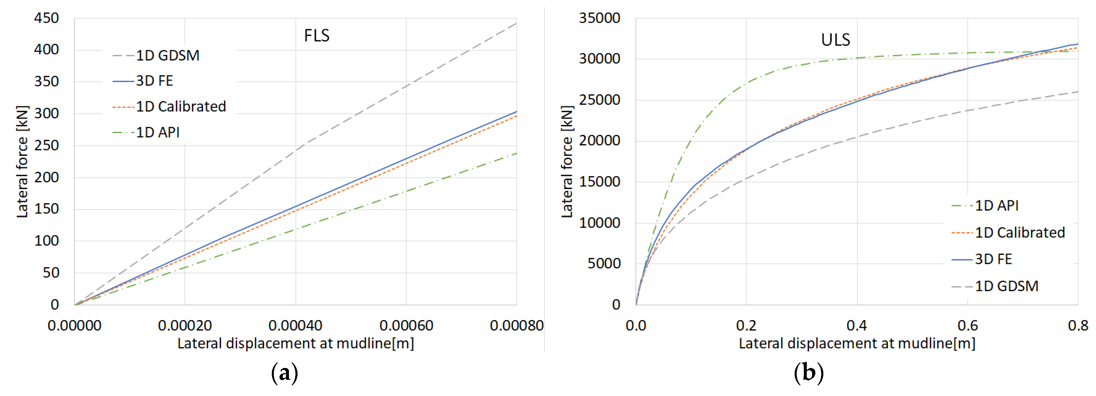
A comparison with the API design method shows a slightly lower ULS bearing capacity but a significantly smaller SLS rotation compared to the 3D FE and 1D Calibrated methods. The slightly lower bearing capacity can be explained by the fact that high friction angles, as present here, are cut-off at 40° in the API method, whereas the high friction angles are taken into account in the other methods. The significantly smaller rotation under SLS conditions (as already mentioned at the end of Section 6) indicates a much higher stiffness in the mid-range of displacements, which can be seen from Figure 8b. This figure shows the load-deflection curves for the different design methods, considering a pile with the designed embedment depth of L = 24 m (based on the 1D Calibrated results for the updated rotation requirement θ = 0.50°). Why the API design method is so much stiffer in the mid-range cannot really be explained from a physical point of view. It is far from the 3D FE results, while the latter are supposed to be most representative of this specific situation.

From the same Figure 8b, it can also be seen that the 1D Calibrated results and the 3D FE results match very well, whereas the overall load-deflection behavior of the GDSM model is less stiff, which confirms the earlier remark that this model has not been calibrated for over-consolidated soil. Nonetheless, the GDSM model could still be used as a first approximation in a concept design study when detailed soil data is absent, whereas it is beneficial to use the PISA numerical based design method (i.c, calibration of 1D model based on 3D FE models) in the final design when more soil data is available.

Although no FLS criteria were formulated for this case, the small displacement diagram in Figure 8a is still interesting to show. In contrast to the right-hand diagram, the 1D GDSM solution is stiffer and the 1D API solution is softer than the 1D Calibrated and 3D FE results for small displacements. The latter can be explained by the fact that the API p-y curves are linear between zero and a substantial fraction of the maximum displacement, while the other solutions involve true small-strain stiffness. This would make the API design method unreliable for FLS design.

8. Conclusions

This paper presents a validation and application of the PLAXIS Monopile Designer (MoDeTo) based on the PISA design method for typical sandy soil as present in the North Sea. After a detailed analysis of the results and a comparison between different design methods, the following conclusions can be summarized:

• Results from the monopile designer, both from 3D finite element calculations as well as from 1D Calibrated soil reactions, are in line with previous results from the PISA research team.
• Although the response from the 1D Calibrated soil reactions is more or less similar as the response from the 3D finite element (FE) calculations, they could be closer if the so-called second-stage optimization would be used to calibrate the soil reactions.
• For normally consolidated sandy soils, as considered in the validation case, the results from the calibrated soil reactions are in line with (although a bit conservative compared to) the results from the General Dunkirk Sand Model (GDSM). For over-consolidated sandy soils, as considered in the application case, the GDSM is more conservative, but could still serve for concept design purposes. Nevertheless, the PISA numerical based design and use of calibrated soil reactions has the advantage of providing a site-specific calibrated response.
• According to the PISA approach, in sandy soils, the SLS design criterion is often decisive as it leads to the largest embedment depth.
• The curve describing the pile rotation as a function of the embedment depth can become rather horizontal near the SLS design criterion. This means, a small reduction in pile rotation requires a significant increase in embedment depth to fulfill the SLS design criterion (if it can be fulfilled at all), which is undesirable. Very competent soil conditions, as considered in [12], seem to be less ‘sensitive’ with respect to the SLS design criterion, although in those cases the SLS criterion still prevails.
• To avoid the undesirable situation as mentioned above, it might be considered to allow for a more relaxed (increased) rotation requirement, since otherwise it may make the monopile unnecessarily expensive. A larger rotation of, for example, 0.50° would seem tolerable, provided the ULS criterion is fulfilled. This would also bring the embedment depth L based on SLS design closer to L based on ULS design.
• Given that the API design method does not explicitly consider the (very) high soil stiffness at small deformations, care must be taken when using this method for FLS design.