Modeling Assessment of Tidal Energy Extraction in the Western Passage


 ,
,  , ,
, ,
Abstract
1. Introduction
2. Methods
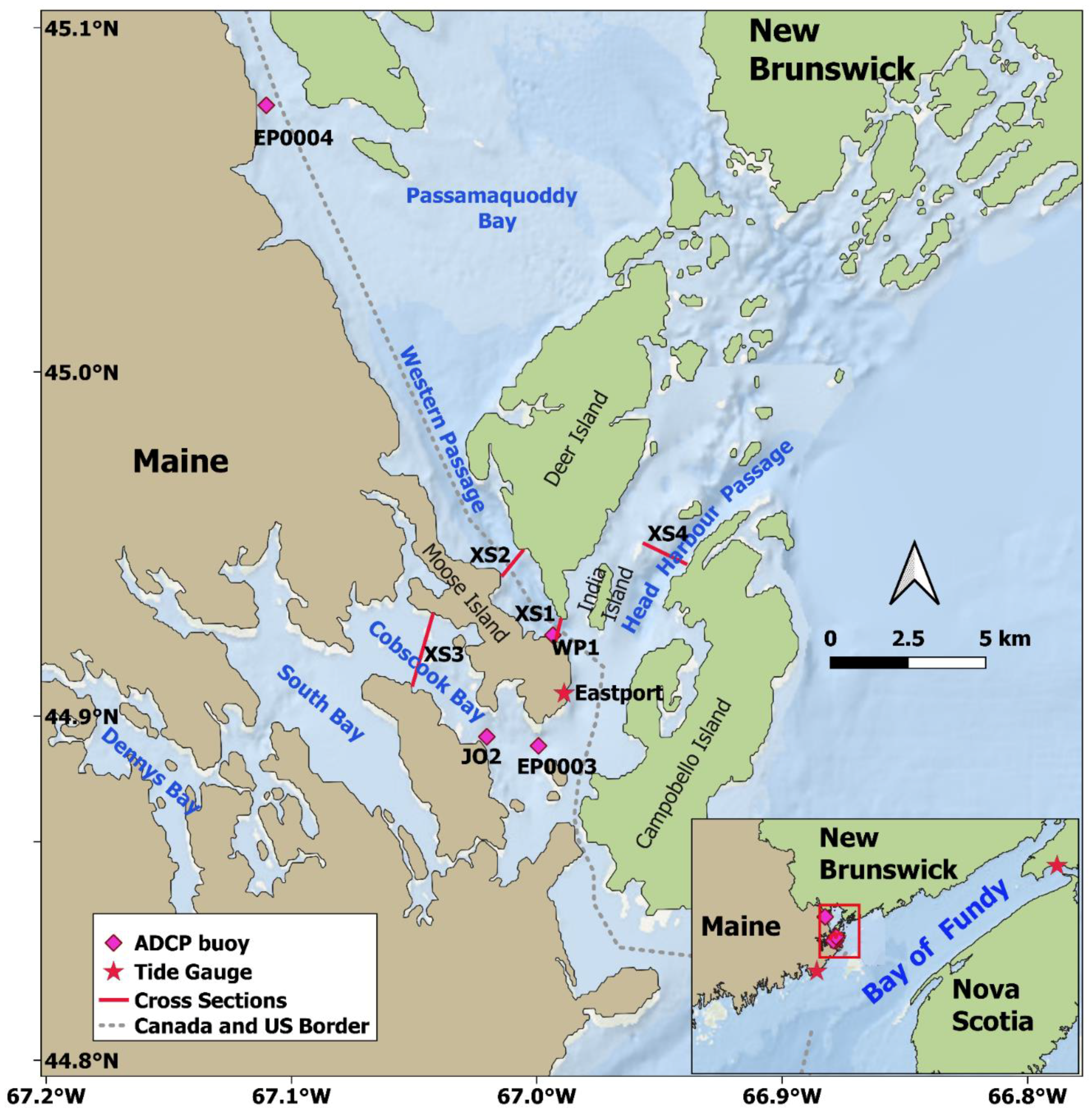
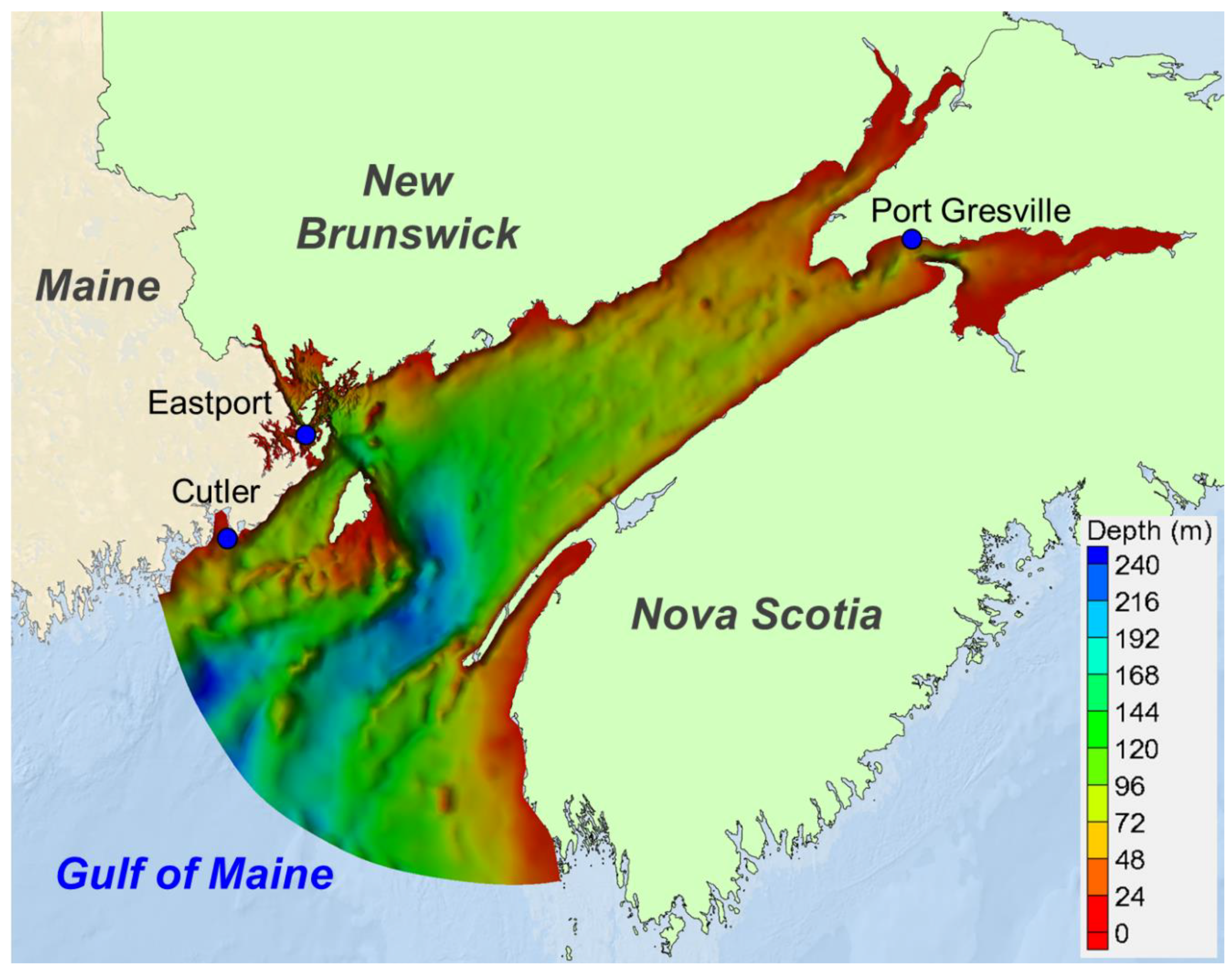
2.1. Study Site
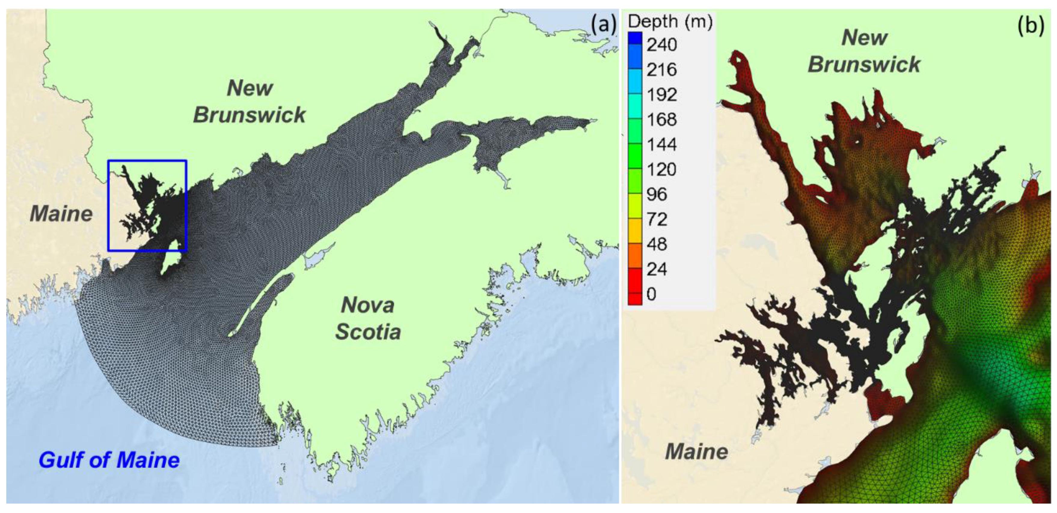
2.2. Tidal Hydrodynamic Model
2.3. Model Configurations and Boundary Conditions
2.4. Observation Data for Model Calibration and Validation
3. Results and Discussion
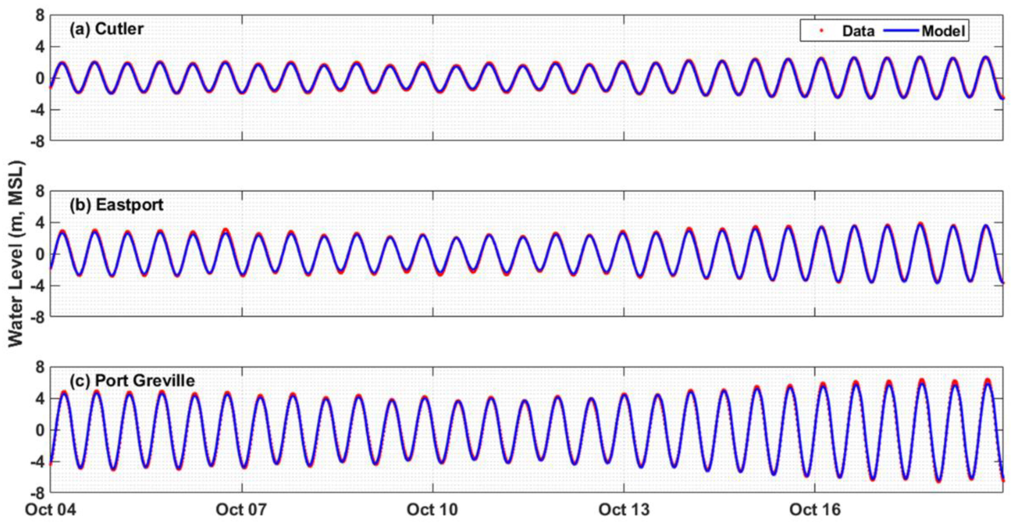
3.1. Model Calibration
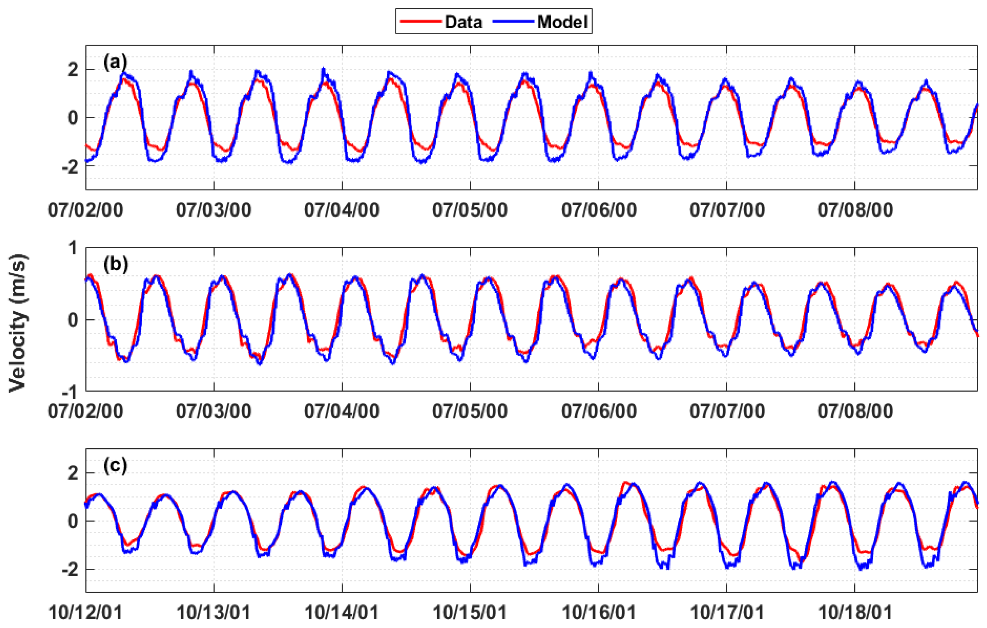
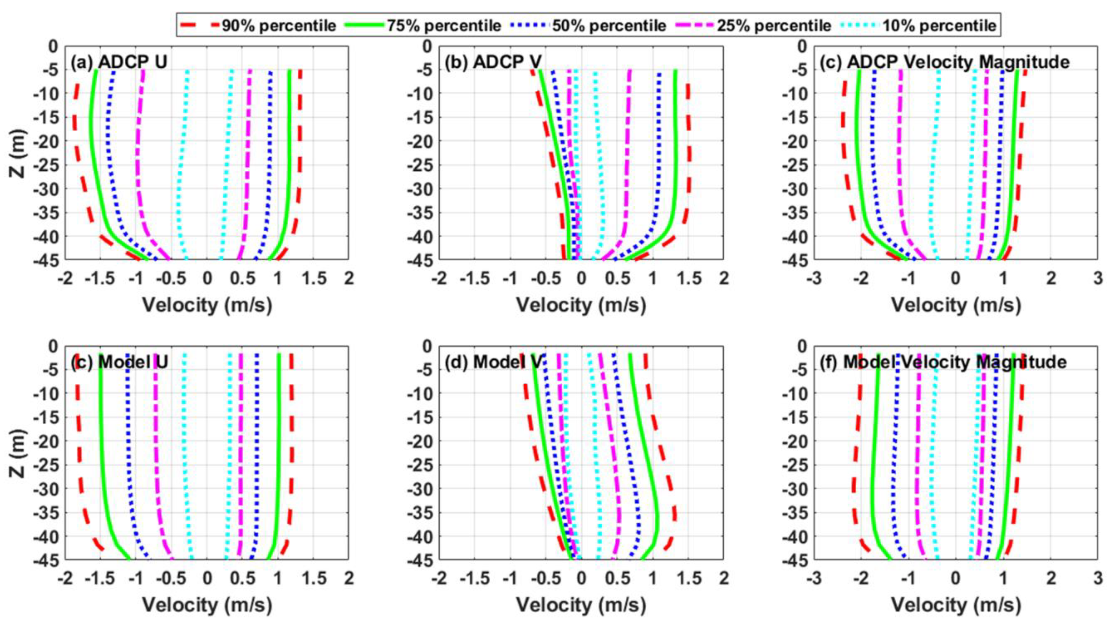
3.2. Model Validation
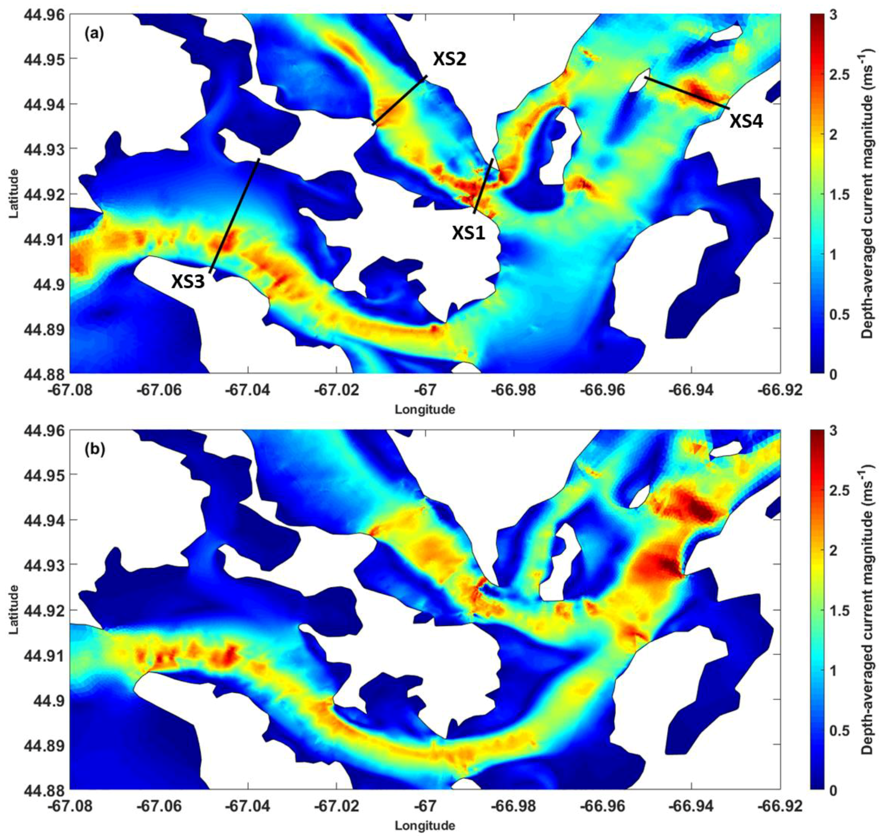
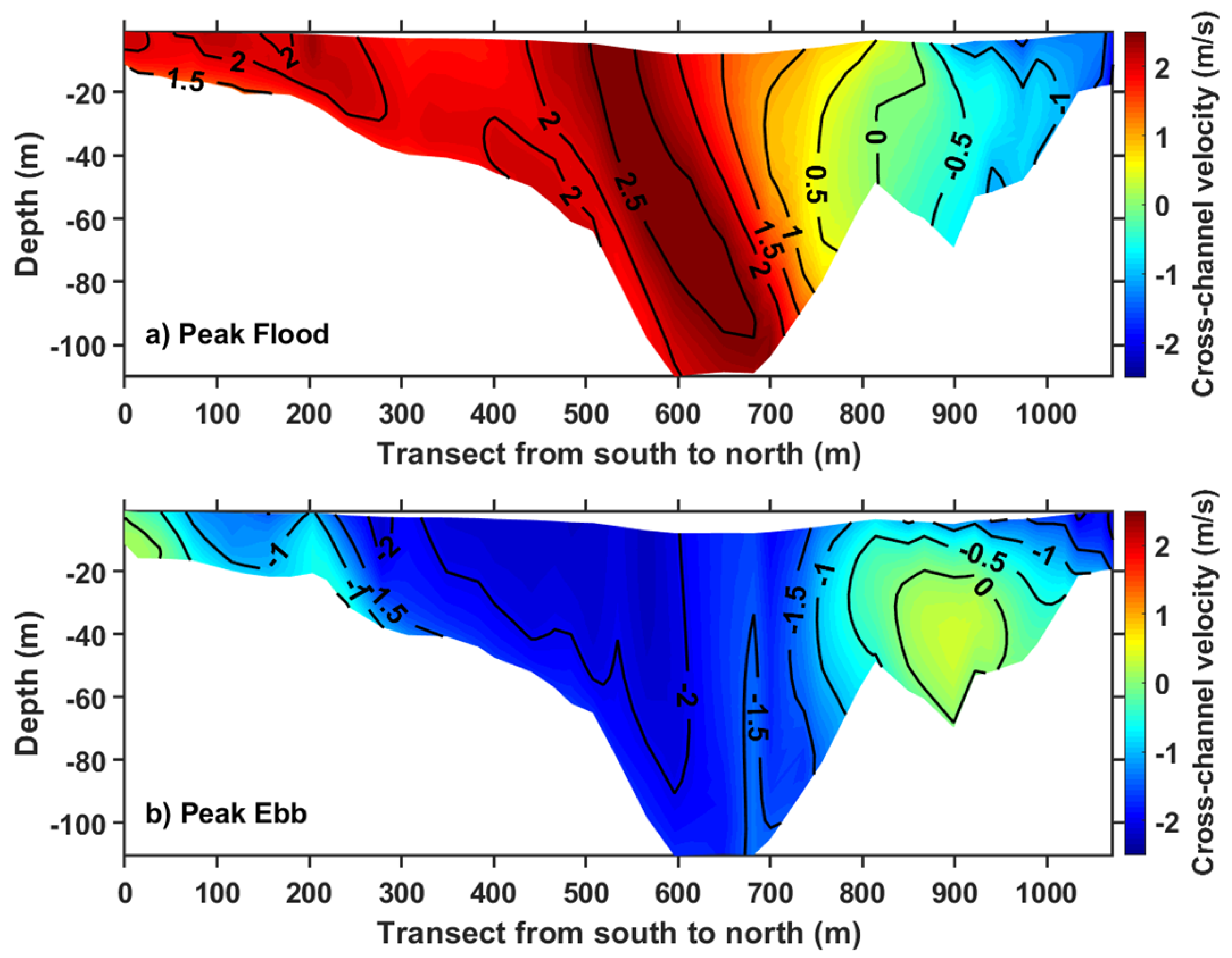
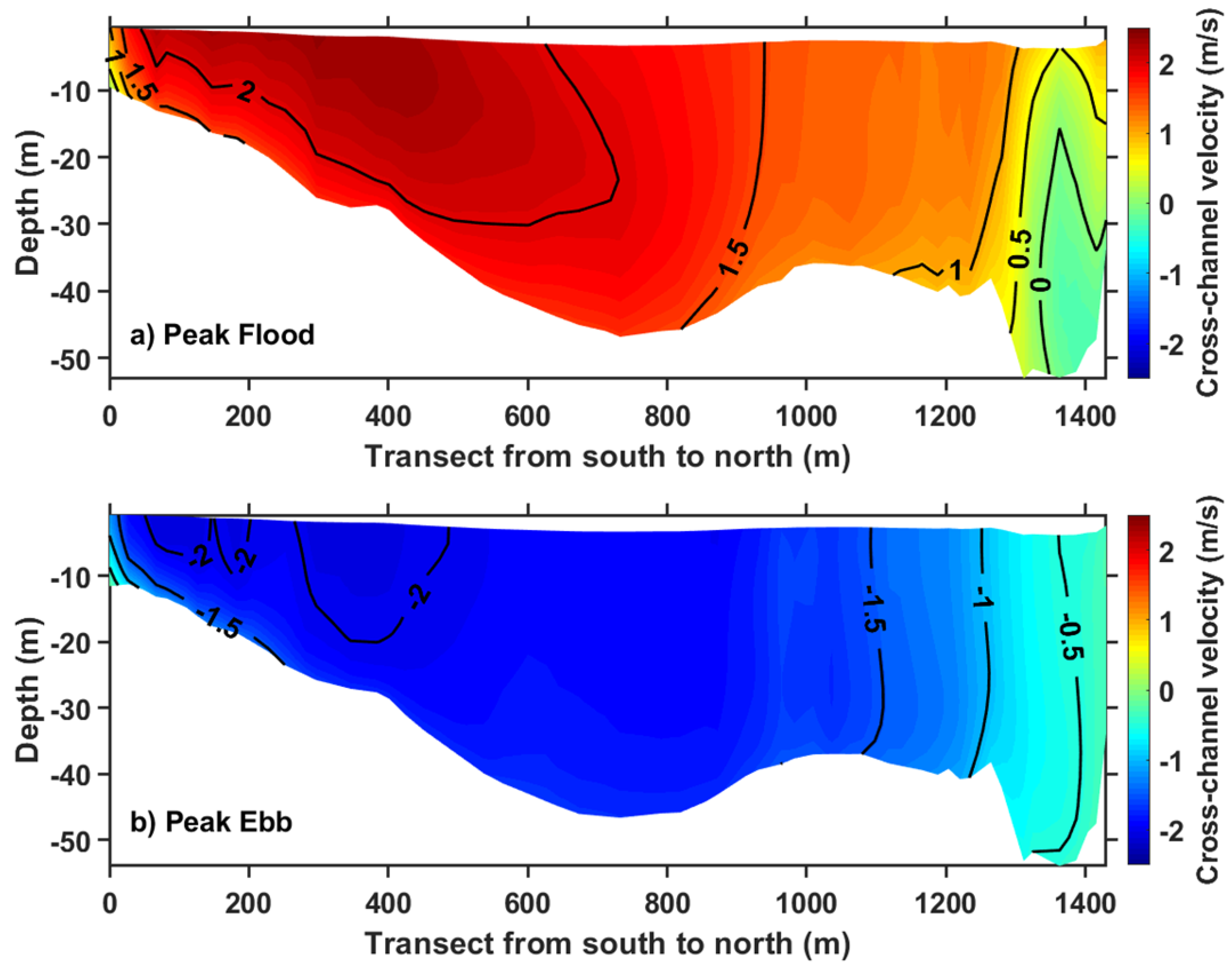
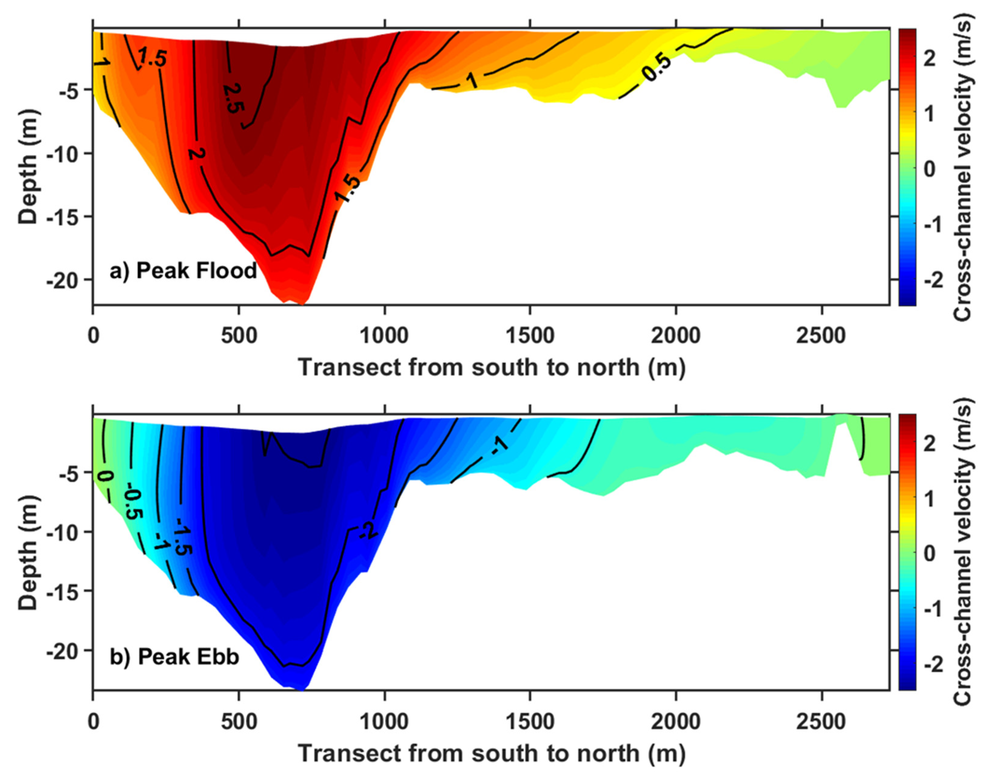
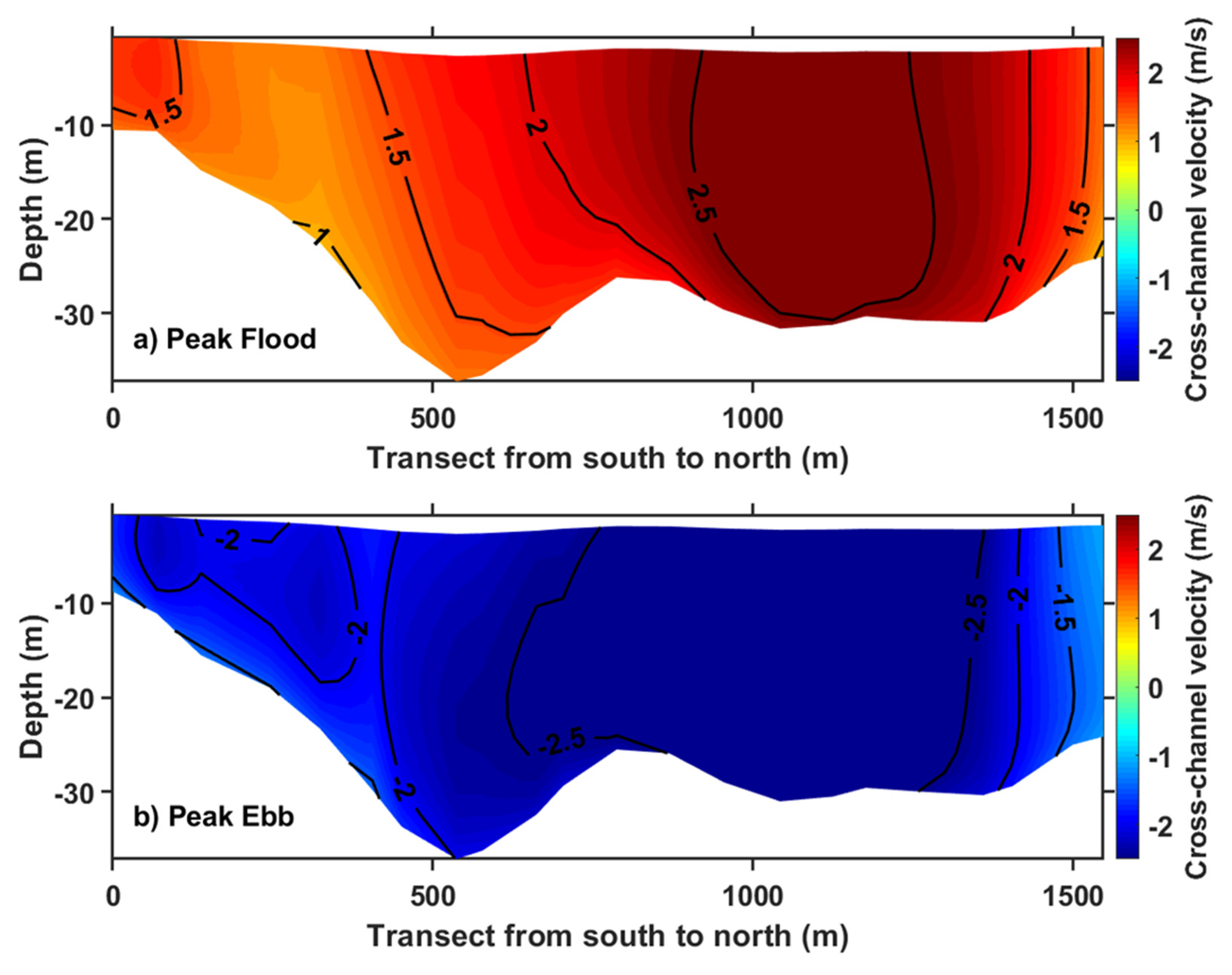
3.3. Characteristics of Tidal Hydrodynamics
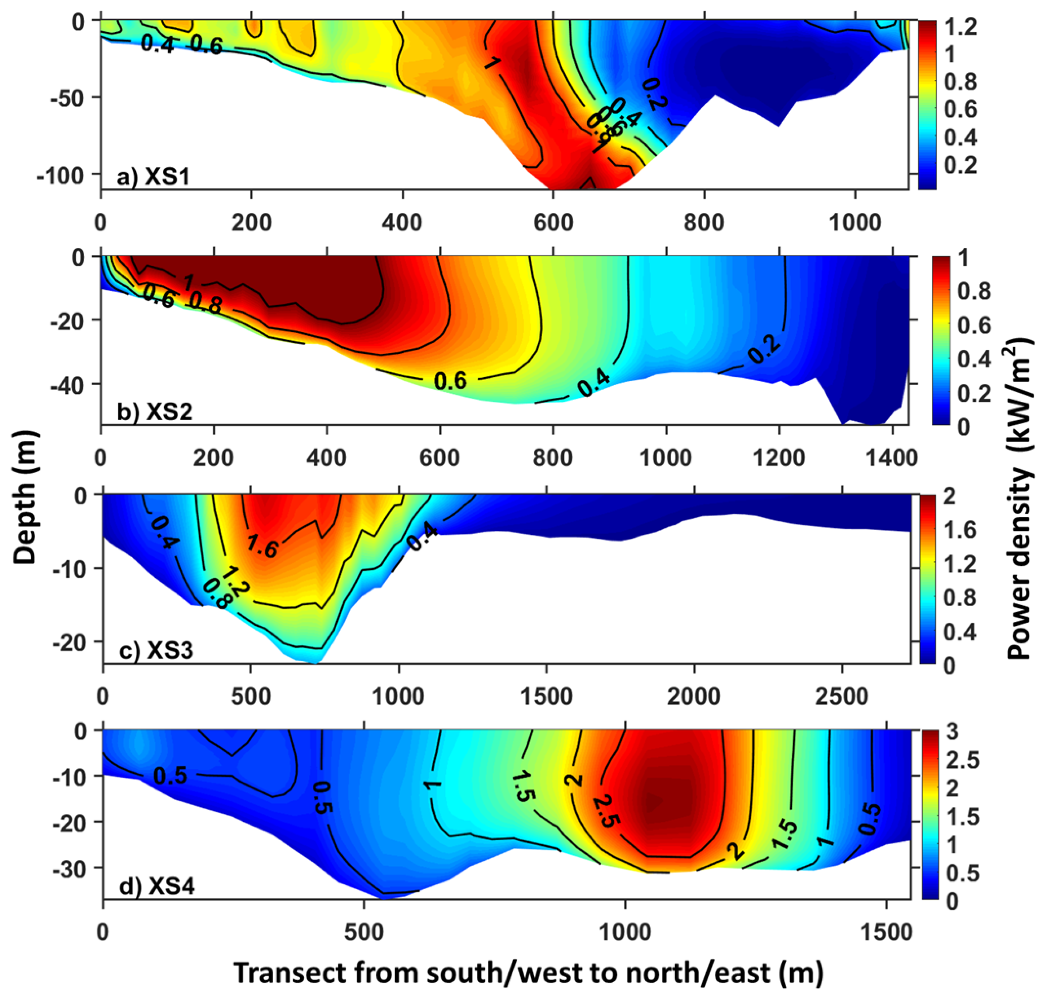
3.4. Along-Channel Kinetic Energy Flux
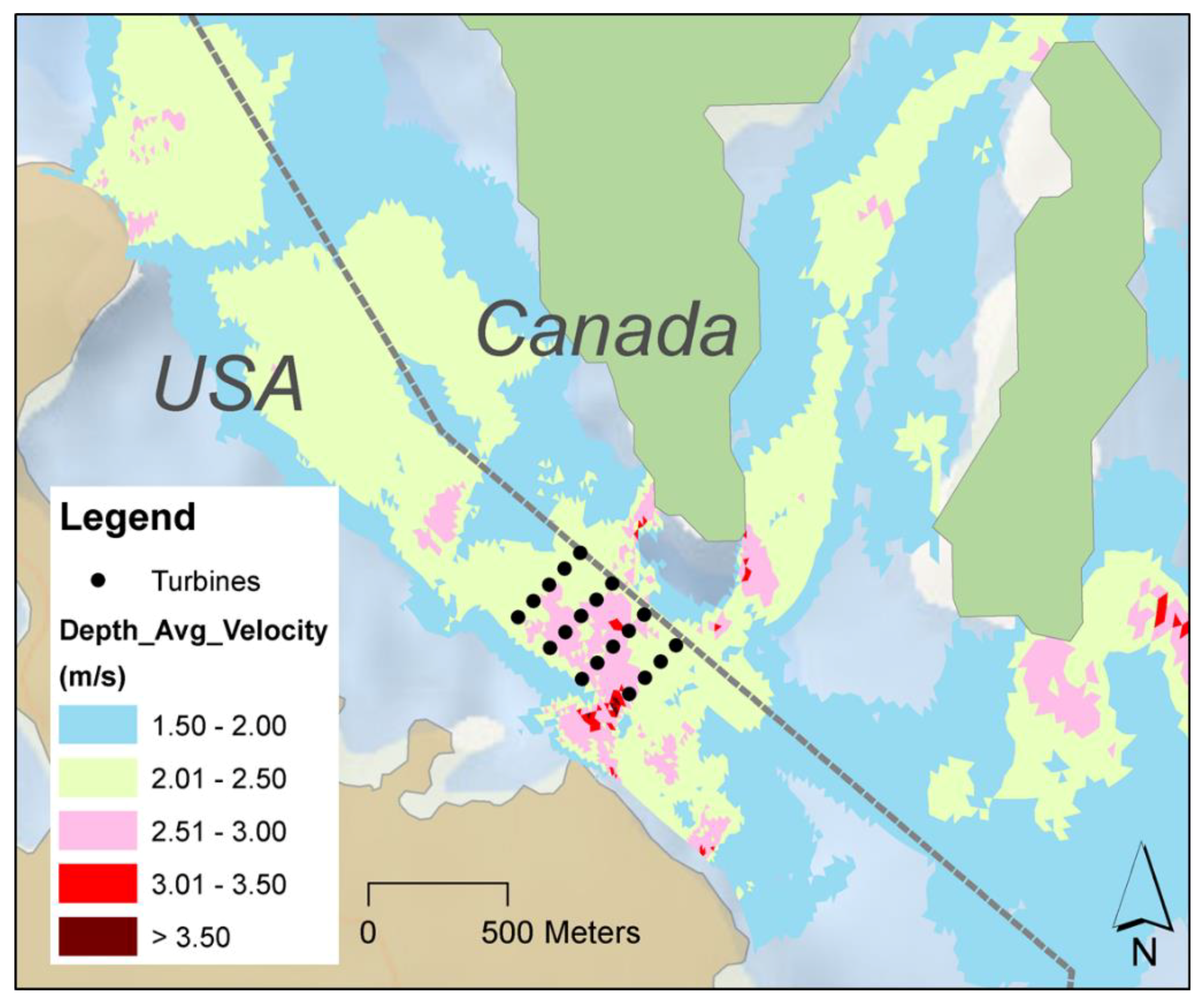
3.5. Energy Extraction in the Western Passage
4. Summary
Author Contributions
Funding
Acknowledgments
Conflicts of Interest
References
- Uihlein, A.; Magagna, D. Wave and tidal current energy—A review of the current state of research beyond technology. Renew. Sustain. Energy Rev. 2016, 58, 1070–1081. [Google Scholar] [CrossRef]
- Bahaj, A.S. New research in tidal current energy. Philos. Trans. R. Soc. A Math. Phys. Eng. Sci. 2013, 371, 20120501. [Google Scholar] [CrossRef] [PubMed][Green Version]
- Bryden, I.G.; Couch, S.I.; Owen, A.; Melville, G. Tidal current resource assessment. Proc. Inst. Mech. Eng. Part A J. Power Energy 2007, 221, 125–135. [Google Scholar] [CrossRef]
- Hussain, A.; Arif, S.M.; Aslam, M. Emerging renewable and sustainable energy technologies: State of the art. Renew. Sustain. Energy Rev. 2017, 71, 12–28. [Google Scholar] [CrossRef]
- Garrett, C.; Cummins, P. The power potential of tidal currents in channels. Proc. R. Soc. A Math. Phys. Eng. Sci. 2005, 461, 2563–2572. [Google Scholar] [CrossRef]
- Garrett, C.; Cummins, P. Maximum power from a turbine farm in shallow water. J. Fluid Mech. 2013, 714, 634–643. [Google Scholar] [CrossRef]
- Yang, Z.Q.; Wang, T.P.; Copping, A.E. Modeling tidal stream energy extraction and its effects on transport processes in a tidal channel and bay system using a three-dimensional coastal ocean model. Renew. Energy 2013, 50, 605–613. [Google Scholar] [CrossRef]
- Blanchfield, J.; Garrett, C.; Wild, P.; Rowe, A. The extractable power from a channel linking a bay to the open ocean. Proc. Inst. Mech. Eng. Part A J. Power Energy 2008, 222, 289–297. [Google Scholar] [CrossRef]
- Bahaj, A.S.; Myers, L. Analytical estimates of the energy yield potential from the Alderney Race (Channel Islands) using marine current energy converters. Renew. Energy 2004, 29, 1931–1945. [Google Scholar] [CrossRef]
- Vennell, R.; Funke, S.W.; Draper, S.; Stevens, C.; Divett, T. Designing large arrays of tidal turbines: A synthesis and review. Renew. Sustain. Energy Rev. 2015, 41, 454–472. [Google Scholar] [CrossRef]
- Adcock, T.A.A.; Draper, S. Power extraction from tidal channels—Multiple tidal constituents, compound tides and overtides. Renew. Energy 2014, 63, 797–806. [Google Scholar] [CrossRef]
- Defne, Z.; Haas, K.A.; Fritz, H.M.; Jiang, L.D.; French, S.P.; Shi, X.; Smith, B.T.; Neary, V.S.; Stewart, K.M. National geodatabase of tidal stream power resource in USA. Renew. Sustain. Energy Rev. 2012, 16, 3326–3338. [Google Scholar] [CrossRef]
- Thiebaut, M.; Filipot, J.F.; Maisondieu, C.; Damblans, G.; Duarte, R.; Droniou, E.; Chaplain, N.; Guillou, S. A comprehensive assessment of turbulence at a tidal-stream energy site influenced by wind-generated ocean waves. Energy 2020, 191, 116550. [Google Scholar] [CrossRef]
- Thiebaut, M.; Sentchev, A.; du Bois, P.B. Merging velocity measurements and modeling to improve understanding of tidal stream resource in Alderney Race. Energy 2019, 178, 460–470. [Google Scholar] [CrossRef]
- Lewis, M.; McNaughton, J.; Marquez-Dominguez, C.; Todeschini, G.; Togneri, M.; Masters, I.; Allmark, M.; Stallard, T.; Neill, S.; Goward-Brown, A.; et al. Power variability of tidal-stream energy and implications for electricity supply. Energy 2019, 183, 1061–1074. [Google Scholar] [CrossRef]
- Wilcox, K.W.; Zhang, J.T.; McLeod, I.M.; Gerber, A.G.; Jeans, T.L.; McMillan, J.; Hay, A.; Karsten, R.; Culina, J. Simulation of device-scale unsteady turbulent flow in the Fundy Tidal Region. Ocean Eng. 2017, 145, 59–76. [Google Scholar] [CrossRef]
- Work, P.A.; Haas, K.A.; Defne, Z.; Gay, T. Tidal stream energy site assessment via three-dimensional model and measurements. Appl. Energy 2013, 102, 510–519. [Google Scholar] [CrossRef]
- Cowles, G.W.; Hakim, A.R.; Churchill, J.H. A comparison of numerical and analytical predictions of the tidal stream power resource of Massachusetts, USA. Renew. Energy 2017, 114, 215–228. [Google Scholar] [CrossRef]
- Marta-Almeida, M.; Cirano, M.; Soares, C.G.; Lessa, G.C. A numerical tidal stream energy assessment study for Baia de Todos os Santos, Brazil. Renew. Energy 2017, 107, 271–287. [Google Scholar] [CrossRef]
- Li, X.R.; Li, M.; McLelland, S.J.; Jordan, L.B.; Simmons, S.M.; Amoudry, L.O.; Ramirez-Mendoza, R.; Thorne, P.D. Modelling tidal stream turbines in a three-dimensional wave-current fully coupled oceanographic model. Renew. Energy 2017, 114, 297–307. [Google Scholar] [CrossRef]
- Yang, Z.; Wang, T.; Copping, A.; Geerlofs, S. Modeling of in-stream tidal energy development and its potential effects in Tacoma Narrows, Washington, USA. Ocean Coast. Manag. 2014, 99, 52–62. [Google Scholar] [CrossRef]
- Sutherland, G.; Foreman, M.; Garrett, C. Tidal current energy assessment for Johnstone Strait, Vancouver Island. Proc. Inst. Mech. Eng. Part A J. Power Energy 2007, 221, 147–157. [Google Scholar] [CrossRef]
- Wang, T.P.; Yang, Z.Q. A modeling study of tidal energy extraction and the associated impact on tidal circulation in a multi-inlet bay system of Puget Sound. Renew. Energy 2017, 114, 204–214. [Google Scholar] [CrossRef]
- Yang, Z.; Wang, T. Modeling the effects of tidal energy extraction on estuarine hydrodynamics in a stratified estuary. Estuaries Coasts 2013, 38, 187–202. [Google Scholar] [CrossRef]
- Wang, T.; Yang, Z.; Copping, A. A modeling study of the potential water quality impacts from in-stream tidal energy extraction. Estuaries Coasts 2013, 38, 173–186. [Google Scholar] [CrossRef]
- Kadiri, M.; Ahmadian, R.; Bockelmann-Evans, B.; Rauen, W.; Falconer, R. A review of the potential water quality impacts of tidal renewable energy systems. Renew. Sustain. Energy Rev. 2012, 16, 329–341. [Google Scholar] [CrossRef]
- IEC. Marine Energy—Wave, Tidal and Other Water Current Converters—Part 201: Tidal Energy Resource Assessment and Characterization; IEC TS 62600-201; International Electrotechnical Commission: Geneva, Switzerland, 2015. [Google Scholar]
- Rao, S.; Xue, H.J.; Bao, M.; Funke, S. Determining tidal turbine farm efficiency in the Western Passage using the disc actuator theory. Ocean Dyn. 2016, 66, 41–57. [Google Scholar] [CrossRef]
- Karsten, R.; Swan, A.; Culina, J. Assessment of arrays of in-stream tidal turbines in the Bay of Fundy. Philos. Trans. R. Soc. A Math. Phys. Eng. Sci. 2013, 371, 20120189. [Google Scholar] [CrossRef]
- Phoenix, A.; Nash, S. Specification of the thrust coefficient when using the momentum sink approach for modelling of tidal turbines. J. Renew. Sustain. Energy 2018, 10, 044502. [Google Scholar] [CrossRef]
- Roc, T.; Conley, D.C.; Greaves, D. Methodology for tidal turbine representation in ocean circulation model. Renew. Energy 2013, 51, 448–464. [Google Scholar] [CrossRef]
- Yang, Z.; Copping, A. Marine Renewable Energy—Resource Characterization and Physical Effects; Springer: Berlin/Heidelberg, Germany, 2017. [Google Scholar]
- Ahmadian, R.; Falconer, R.; Bockelmann-Evans, B. Far-field modelling of the hydro-environmental impact of tidal stream turbines. Renew. Energy 2012, 38, 107–116. [Google Scholar] [CrossRef]
- Kilcher, K.; Thresher, R.; Tinnesand, H. Marine Hydrokinetic Energy Site Identification and Ranking Methodology Part II: Tidal Energy; National Renewable Energy Laboratory: Golden, CO, USA, 2016; p. 30.
- Brooks, D.A. The tidal-stream energy resource in Passamaquoddy-Cobscook Bays: A fresh look at an old story. Renew. Energy 2006, 31, 2284–2295. [Google Scholar] [CrossRef]
- Amante, C.; Eakins, B.W. ETOPO1 1 Arc-Minute Global Relief Model: Procedures, Data Sources and Analysis; NOAA Technical Memorandum NESDIS NGDC-24 2009; National Geophysical Data Center, NOAA: Boulder, CO, USA, 2009.
- Chen, C.; Liu, H.; Beardsley, R.C. An unstructured grid, finite-volume, three-dimensional, primitive equations ocean model: Application to coastal ocean and estuaries. J. Atmos. Ocean. Technol. 2003, 20, 159–186. [Google Scholar] [CrossRef]
- Chen, C.B.; Robert, C.; Cowles, G. An unstructured grid, finite-volume coastal ocean model (FVCOM) system. Oceanography 2006, 19, 78–89. [Google Scholar] [CrossRef]
- Mellor, G.L.; Yamada, T. Development of a turbulence closure-model for geophysical fluid problems. Rev. Geophys. 1982, 20, 851–875. [Google Scholar] [CrossRef]
- Xuan, J.; Yang, Z.; Huang, D.; Wang, T.; Zhou, F. Tidal residual current and its role in the mean flow on the Changjiang Bank. J. Mar. Syst. 2016, 154, 66–81. [Google Scholar] [CrossRef]
- Lai, Z.; Ma, R.; Gao, G.; Chen, C.; Beardsley, R.C. Impact of multichannel river network on the plume dynamics in the Pearl River estuary. J. Geophys. Res. Ocean. 2015, 120, 5766–5789. [Google Scholar] [CrossRef]
- Chen, T.Q.; Zhang, Q.H.; Wu, Y.S.; Ji, C.; Yang, J.S.; Liu, G.W. Development of a wave-current model through coupling of FVCOM and SWAN. Ocean Eng. 2018, 164, 443–454. [Google Scholar] [CrossRef]
- Xiao, Z.Y.; Wang, X.H.; Roughan, M.; Harrison, D. Numerical modelling of the Sydney Harbour Estuary, New South Wales: Lateral circulation and asymmetric vertical mixing. Estuar. Coast. Shelf Sci. 2019, 217, 132–147. [Google Scholar] [CrossRef]
- Khangaonkar, T.; Sackmann, B.; Long, W.; Mohamedali, T.; Roberts, M. Simulation of annual biogeochemical cycles of nutrient balance, phytoplankton bloom(s), and DO in Puget Sound using an unstructured grid model. Ocean Dyn. 2012, 62, 1353–1379. [Google Scholar] [CrossRef]
- Khangaonkar, T.; Nugraha, A.; Hinton, S.; Michalsen, D.; Brown, S. Sediment transport into the Swinomish Navigation Channel, Puget Sound—Habitat restoration versus navigation maintenance needs. J. Mar. Sci. Eng. 2017, 5, 19. [Google Scholar] [CrossRef]
- Luo, L.; Wang, J.; Schwab, D.J.; Vanderploeg, H.; Leshkevich, G.; Bai, X.Z.; Hu, H.G.; Wang, D.X. Simulating the 1998 spring bloom in Lake Michigan using a coupled physical-biological model. J. Geophys. Res. Ocean. 2012, 117. [Google Scholar] [CrossRef]
- Hakim, A.R.; Cowles, G.W.; Churchill, J.H. The impact of tidal stream turbines on circulation and sediment transport in Muskeget Channel, MA. Mar. Technol. Soc. J. 2013, 47, 122–136. [Google Scholar] [CrossRef]
- Yang, Z.Q.; Wang, T.P.; Leung, R.; Hibbard, K.; Janetos, T.; Kraucunas, I.; Rice, J.; Preston, B.; Wilbanks, T. A modeling study of coastal inundation induced by storm surge, sea-level rise, and subsidence in the Gulf of Mexico. Nat. Hazards 2014, 71, 1771–1794. [Google Scholar] [CrossRef]
- Wang, T.P.; Yang, Z.Q. The nonlinear response of storm surge to sea-level rise: A modeling approach. J. Coast. Res. 2019, 35, 287–294. [Google Scholar] [CrossRef]
- Yoon, J.J.; Shim, J.S. Estimation of storm surge inundation and hazard mapping for the southern coast of Korea. J. Coast. Res. 2013, 65 (Suppl. 1), 856–861. [Google Scholar] [CrossRef]
- Ge, J.; Much, D.; Kappenberg, J.; Nino, O.; Ding, P.; Chen, Z. Simulating storm flooding maps over HafenCity under present and sea level rise scenarios. J. Flood Risk Manag. 2014, 7, 319–331. [Google Scholar] [CrossRef]
- Chen, C.S.; Beardsley, R.C.; Luettich, R.A.; Westerink, J.J.; Wang, H.; Perrie, W.; Xu, Q.C.; Donahue, A.S.; Qi, J.H.; Lin, H.C.; et al. Extratropical storm inundation testbed: Intermodel comparisons in Scituate, Massachusetts. J. Geophys. Res. Ocean. 2013, 118, 5054–5073. [Google Scholar] [CrossRef]
- Egbert, G.D.; Erofeeva, S.Y. Efficient inverse modeling of barotropic ocean tides. J. Atmos. Ocean. Technol. 2002, 19, 183–204. [Google Scholar] [CrossRef]
- Murray, R.O.; Gallego, A. A modelling study of the tidal stream resource of the Pentland Firth, Scotland. Renew. Energy 2017, 102, 326–340. [Google Scholar] [CrossRef]
- Haverson, D.; Bacon, J.; Smith, H.C.M.; Venugopal, V.; Xiao, Q. Modelling the hydrodynamic and morphological impacts of a tidal stream development in Ramsey Sound. Renew. Energy 2018, 126, 876–887. [Google Scholar] [CrossRef]
- Plew, D.R.; Stevens, C.L. Numerical modelling of the effect of turbines on currents in a tidal channel—Tory Channel, New Zealand. Renew. Energy 2013, 57, 269–282. [Google Scholar] [CrossRef]


| Station | Type | Longitude | Latitude | Depth (m) | Year |
|---|---|---|---|---|---|
| Eastport, ME | Tide Gage | −66.985 | 44.903 | 6.7 | 2000 |
| Cutler, ME | XTide | −64.967 | 45.567 | 5.9 | 2000 |
| Port Greville, NS | XTide | −64.550 | 45.400 | 11.8 | 2000 |
| EP0003 | ADCP | −66.996 | 44.888 | 34.1 | 2000 |
| EP0004 | ADCP | −67.101 | 45.076 | 32.0 | 2000 |
| JO2 | ADCP | −67.017 | 44.891 | 32.0 | 2001 |
| WP1 | ADCP | −66.989 | 44.920 | 45.0 | 2017 |
| Water Level | Cutler | Eastport | Port Greville |
|---|---|---|---|
| RMSE (m) | 0.15 | 0.26 | 0.41 |
| SI | 0.12 | 0.15 | 0.13 |
| R2 | 0.99 | 0.99 | 0.99 |
| Depth-Average Velocity | EP0003 | EP0004 | J02 |
|---|---|---|---|
| RMSE (m/s) | 0.38 | 0.14 | 0.27 |
| SI | 0.42 | 0.41 | 0.33 |
| R2 | 0.97 | 0.94 | 0.96 |
| Water Level (m) | M2 | N2 | S2 | K1 | O1 | P1 | Q1 | M6 | MK3 | MS4 |
|---|---|---|---|---|---|---|---|---|---|---|
| Data (WP1) | 2.72 | 0.38 | 0.54 | 0.09 | 0.14 | 0.06 | 0.06 | 0.15 | 0.02 | 0.18 |
| Model | 2.62 | 0.38 | 0.52 | 0.08 | 0.15 | 0.06 | 0.02 | 0.17 | 0.02 | 0.09 |
| Difference | −0.11 | 0.01 | −0.03 | −0.01 | 0.01 | 0.01 | −0.04 | 0.03 | 0.00 | −0.09 |
| Percentage Error | 3.9 | 1.5 | 4.8 | 10.9 | 5.4 | 12.8 | 66.9 | 18.7 | 3.1 | 53.3 |
| Current (m/s) | M2 | N2 | S2 | K1 | O1 | P1 | Q1 | M6 | MK3 | MS4 |
|---|---|---|---|---|---|---|---|---|---|---|
| Data (WP1) | 1.67 | 0.25 | 0.34 | 0.07 | 0.04 | 0.21 | 0.11 | 0.07 | 0.06 | 0.12 |
| Model | 1.46 | 0.23 | 0.31 | 0.04 | 0.04 | 0.20 | 0.04 | 0.06 | 0.04 | 0.03 |
| Difference | −0.21 | −0.02 | −0.03 | −0.02 | −0.01 | −0.01 | −0.07 | −0.01 | −0.02 | −0.09 |
| Percentage Error | 12.4 | 8.5 | 7.8 | 32.1 | 13.9 | 3.9 | 62.9 | 13.2 | 26.6 | 71.9 |
| Total Turbines | Turbine Spacing | Hub Height | Turbine Diameter | Avg. Extracted Power (kW) | Power per Turbine (kW) |
|---|---|---|---|---|---|
| 19 | 80 m × 160 m | 15 m | 20 m | 4810 | 253 |
© 2020 by the authors. Licensee MDPI, Basel, Switzerland. This article is an open access article distributed under the terms and conditions of the Creative Commons Attribution (CC BY) license (http://creativecommons.org/licenses/by/4.0/).
Share and Cite
Yang, Z.; Wang, T.; Xiao, Z.; Kilcher, L.; Haas, K.; Xue, H.; Feng, X. Modeling Assessment of Tidal Energy Extraction in the Western Passage. J. Mar. Sci. Eng. 2020, 8, 411. https://doi.org/10.3390/jmse8060411
Yang Z, Wang T, Xiao Z, Kilcher L, Haas K, Xue H, Feng X. Modeling Assessment of Tidal Energy Extraction in the Western Passage. Journal of Marine Science and Engineering. 2020; 8(6):411. https://doi.org/10.3390/jmse8060411
Chicago/Turabian StyleYang, Zhaoqing, Taiping Wang, Ziyu Xiao, Levi Kilcher, Kevin Haas, Huijie Xue, and Xi Feng. 2020. "Modeling Assessment of Tidal Energy Extraction in the Western Passage" Journal of Marine Science and Engineering 8, no. 6: 411. https://doi.org/10.3390/jmse8060411
APA StyleYang, Z., Wang, T., Xiao, Z., Kilcher, L., Haas, K., Xue, H., & Feng, X. (2020). Modeling Assessment of Tidal Energy Extraction in the Western Passage. Journal of Marine Science and Engineering, 8(6), 411. https://doi.org/10.3390/jmse8060411