Uncertainty Analysis of Ship Model Propulsion Test on Actual Seas Based on Monte Carlo Method

Abstract

As a new testing technology, large-scale ship model tests on the sea are advantageous in addressing the scale effect in ship models and in simulating ship navigation conditions. In this study, the uncertainty of a ship model propulsion test on the sea was analyzed using the Monte Carlo method, and the influence of the test environment was quantified. We used a 25 m-long ship model for the propulsion performance test. Based on the procedure recommended by the International Standardization Organization (ISO), several tests were conducted on the Yellow Sea (the northwestern part of the East China Sea). The results demonstrate that the wind and waves in the environment are the two factors that have the greatest influence on the test accuracy. This study will aid the development of sea trials, and the analysis method used in the propulsion test is also suitable for many complex ship tests.

1. Introduction

The propulsion test of ship models on actual seas is a test performed using a large-scale model in a natural water environment. The test site is selected in an offshore area where the wind, waves, and currents are similar to the navigation conditions of a real ship. This ensures that the performance of the ship propulsion system can be predicted more accurately. Since the test object is a large-scale model, such tests can also effectively alleviate the scale effect in the towing-tank tests, so as to improve the accuracy of extrapolation calculation. It also significantly saves manpower, materials, and financial resources compared to tests using a full-scale ship, so that repeated tests can be carried out. In addition, it is difficult to modify the full real ship once it has been built and launched. Hence, the method has broad development prospects. However, as this kind of test technology is still in the exploratory stage and there is insufficient comparative research data, it is necessary to evaluate the uncertainty of the test to determine the reliability of its scheme and the validity of the measurement data.

Uncertainty indicates the degree of trust in the measurement results. For the ship model test, the International Towing Tank Conference (ITTC) initially followed the American Institute of Aeronautics and Astronautics (AIAA) standard (1995) to analyze the uncertainty from the viewpoint of bias and precision errors [1,2]. Stern et al. provided a summary of the AIAA standard for the experimental uncertainty assessment methodology [3]. They assert that the benefits of uncertainty analysis far outweigh the time it takes to evaluate measurement results. Subsequently, concomitant with the widespread application of the “Guide to the Expression of Uncertainty in Measurement (GUM)” around the world [4], the uncertainty Analysis Committee of ITTC also voted in to recommend the use of this method to evaluate relevant experiments [5]. In order to compare the characteristics of the old and new methods, Delen et al. used two ITTC (2002 and 2014) procedures based on different standards to analyze the uncertainty of ship model resistance tests in towing tanks [6]. With the gradual improvement of the uncertainty analysis method of resistance tests, Nikolov et al. studied the uncertainty of tow-tank testing of high-speed planning craft, in order to generate more data to incorporate into the evaluation process [7].

The test sites used in the above studies were all in towing tanks, and most of them evaluated resistance tests. With the diversification of the experimental environment and the complexity of the computational model, the traditional rules based on the Taylor series method (TSM) cannot fully meet the present evaluation needs [8]. Recently, several scholars have used the Monte Carlo method (MCM) to study the uncertainty of ship tests, especially for trials on actual seas. For example, Insel analyzed the navigation test of a group of sister ships at sea by utilizing the ITTC standard speed/powering trial analysis procedure with Monte Carlo simulations, with particular focus on the influence of the Beaufort scale and other uncertainty factors [9]. Kamal introduced the MCM into the extrapolation prediction of dynamic ship performances [10]. By referring to the ITTC1978 procedure, the uncertainty caused by the error source in the resistance and propulsion test was studied. Samples were taken from the existing sea trial and towing tank test, and the uncertainty of the system was calculated. Woodward analyzed the uncertainty of the maneuverability test of the ship model, showed the transfer process of the uncertainty component by the MCM, and determined the error source [11,12]. Subsequently, Vrijdag compared the advantages and disadvantages of the linear method and the MCM in ship performance prediction and analyzed the factors that significantly influence ship speed and bollard pull predictions [13]. Gavrilin analyzed the maneuvering sea trial results of the ship “Gunnerus” and proposed a method to evaluate the uncertainty of test results caused by environmental impact using a simulation model based on the MCM [14]. Aldous detailed and categorized the relevant sources of uncertainty in performance measurements and proposed a method to quantify the overall uncertainty on a ship performance indicator based on the MCM [15]. A sensitivity analysis was also conducted on the sources of uncertainty to highlight the relative importance of each source. Seo studied the speed and power performance results of real ships using the MCM [16]. Based on the correction method of real ship data published by the ISO, the Monte Carlo results were approximated to the normal distribution, and the uncertain sources under actual sea conditions were analyzed.

This present study was conducted with the objective of using prototype ships to perform the tests. However, for ship model propulsion tests on real seas, there is no relevant uncertainty evaluation data. Therefore, in this study, according to the methodology recommended by the ISO, the uncertainty of large-scale ship model propulsion tests on actual seas was evaluated and analyzed based on the Monte Carlo numerical simulation method. The uncertainty of the environment and propulsion efficiency were also simulated and calculated using an adaptive program.

The aim is to quantify the uncertainty caused by various factors in the test through the analysis of a ship model propulsion test on actual seas, so as to obtain the influence of different error sources on the measurement accuracy. The main part of this study is to analyze the interference of the test environment and discuss the influence of wind wave and current. At the same time, the uncertainty variation trend caused by wind and waves of different degrees was simulated through the program, which provided data reference for similar experiments and clarified the direction of further work.

2. Materials and Methods

2.1. Methods

Presently, there are two main evaluation methods in the field of measurement uncertainty. One is the traditional Taylor series method. The initial concept of bias and precision error and the type A and B methods are based on the Taylor series method. The other method is the MCM, which involves the use of a computer to record a large number of samples from the assumed distribution and then repeated execution of the test simulations to obtain the evaluation uncertainty [8].

2.1.1. Guide to the Expression of Uncertainty in Measurement (GUM, Based on Taylor Series Method)

In most cases, the final result Y cannot be obtained directly but is determined from N other quantities X₁, X₂,…, X_N through a functional relationship f:

$$Y=f(X_1,X_2,\dots ,X_N).$$

(1)

The definition of f expresses the entire measurement process and includes all the quantities that may lead to the uncertainty of Y. According to the Joint Committee for Guides in Metrology (JCGM), uncertainty can be divided into three categories: standard, combined, and expanded [4].

The value of the standard uncertainty u is equal to the positive square root of the estimated variance. To facilitate the distinction, the GUM method is divided into types A and B according to different evaluation methods. Among them, type A represents the uncertainty components obtained by the statistical analysis of a series of observed data, while the components obtained by the other methods are classified as type B.

The combined standard uncertainty is evaluated based on the transfer rule of uncertainty, and the correlation between variables was not considered in this study. Thus, the equation can be expressed as follows:

$$u_c{}^2(y)={\displaystyle \sum _{i=1}^N{c}_i{}^2{u}^2(x_i)},$$

(2)

where c_i represents the sensitivity coefficient. In some applications, it is often necessary to provide a measure of uncertainty; that is, an interval containing most of the data. The formula for calculating the expanded uncertainty is as follows:

$$U=k{u}_c(y).$$

(3)

Generally, k ranges from 2 to 3, and for normal distribution functions, k = 2 corresponds to an inclusion probability of approximately 95.45%. In addition, to express the degree of deviation of the data more clearly, this study added the concept of relative uncertainty to the evaluation.

2.1.2. Monte Carlo Method (MCM)

The MCM is a supplementary document for the GUM proposed by the JCGM, which can solve some complex non-linear problems [17]. The point of this method is to repeatedly sample the probability density function of the input X_i. The main implementation steps of the adaptive MCM are as follows:

• Initialize the parameter setting.
• Establish the model according to the data reduction and set the distribution of the input.
• Use the computer to simulate the output object.
• Use the stability judgment program to judge whether the output meets the requirement of numerical tolerance.
• Obtain the final report.

2.2. Sea Trials

2.2.1. Ship Model

The full-scale ship of this test was the 230000DWT ‘CSB FORTUNE’, and the main body of the model’s shell was made of fiberglass. The ship model is shown in Figure 1.

The main parameters of the ship model are listed in

Table 1. Main parameters of the ship model.

LOA (m)	LWL (m)	Lpp (m)	B (m)	D (m)	D (m)	S (m2)	∇ (m3)	λ
24.99	24.62	24.20	4.04	1.87	1.39	144.75	115.20	1:13

.

2.2.2. Test Process

The propulsion test site was a sea in Qingdao, China. To meet the approximate requirements of sea conditions set in ISO, the test was performed when the wind and waves were mild [18]. To reduce the blocking effect, the experiment was performed at the time of the day when the tide rose above half tide.

The test contents included the measurement and analysis of the wind, wave, and current at sea, the motion attitude of the ship model in the wind and waves, and the hydrodynamic performance of the propeller. Among them, the test contents of wind, wave, and current included the wind speed, wind direction, wave height, and current parameters. The motion attitude test content mainly included the navigation trajectory, roll, and trim and acceleration of the head and tail of the ship model. The propeller test content included its thrust and torque.

Before the test, it was necessary to conduct preparatory work in the wharf, including adjusting the floating state and debugging the measuring instruments, as shown in Figure 2a. After waiting for the water level to rise, the auxiliary ship assisted with leaving the port and towing the main ship to the designated offshore test area, as shown in Figure 2b.

The propulsion test, which followed the procedure recommended by ISO 15016(2015) [18], can be divided into the following steps:

• The experimenter observes the waves and chooses a suitable sailing direction according to the direction of the waves.
• Before the test, the propeller is rotated at a very slow speed (1 r/min) to obtain the initial values of the shafting thrust and torque.
• The ship model accelerates from the starting point to the speed under the specified working conditions until the speed of the propeller is stable. The test conditions are converted from the sailing parameters of the prototype ship.
• For each test condition, it is necessary for the ship model to sail in a constant state long enough, and then the steering system turns the ship bow to make the model go back in the reverse direction parallel to the test baseline to conduct another test and record the test data.
• Because of the low speed of the model in this test, the test under different working conditions can be performed in one direct voyage. The ship model should sail for enough time under each working condition, which effectively reduces the time loss of its turning.
• To correct the influence of current, the above experiments need to be repeated according to the correction method. The actual propulsion test is shown in Figure 2c.
• After completing several tests, it is necessary to check the gasoline consumption of the generator. If it is found that the fuel is used up, the power supply should be disconnected in time, and the fuel should be replenished after the environment in the cockpit is more stable, as shown in Figure 2d.

3. Results

Similar to the towing tank test, uncertainty analysis of the propulsion test on an actual sea requires consideration of the geometric structure uncertainty of the ship model, installation of equipment, and measurement of related quantities, where the Taylor series method can be used in this part. In addition, because the experiment was performed under actual sea conditions, it is necessary to consider the interference of wind, wave, and current in the environment. The fluctuation of these factors in the entire test process suggests non-linear characteristics, and the related correction formula is complex. Thus, in this study, the MCM was used to evaluate the uncertainty.

3.1. Uncertainty of Ship Model

The uncertainty of the ship model conditions can be divided into the following parts [18]:

• Before each sea test, the floating state of the ship model requires adjustments in the wharf, and the relative error of displacement is generally required to be less than 2%. In this test, the estimated error of the displacement of the ship model was 1000 kg, and the relative deviation was about 1%.
• The trim condition of the ship model is an important parameter for the test, but it does not consider the final range of uncertainty evaluation. Generally, the trim is less than 0.1% of the length between the vertical lines, and the error of the bow draught within a range of ± 0.1 m can be considered to meet the test requirements.
• During ship navigation, the hull roughness or growth of marine life will significantly increase the resistance of the ship. Presently, there is no accurate correction method in this respect. Hence, the hull and propeller require a careful check before the test. The ship model in this experiment spent a short time at sea, and it was observed that the surface of the propeller was relatively smooth when the propeller was dismantled in the middle of the test. Thus, the influence of roughness was ignored.

3.2. Uncertainty of Shafting Measuring Instrument

In this test, the torque and thrust of the shafting were measured by a special self-propulsion instrument in which the torque measuring device was a T40B (HBM) digital torque sensor with a measuring range of 500 Nm, and the measuring accuracy was 0.25 Nm. The measuring accuracy of the force sensor used in the thrust was 2 N. The shafting motor was a Siemens motor, which offers a high precision and a rotational speed precision of 0.5 rpm. The standard uncertainty of the parameters in the shafting can thus be expressed as follows, the coverage factor k corresponding to the instrument is 3:

$$\begin{array}{l}u(Q)=0.25 \mathrm{Nm}/3=0.083 \mathrm{Nm}\\ u(T)=4 \mathrm{N}/3=1.3 \mathrm{N}\\ u(n)=0.5 \mathrm{rpm}/3=0.167 \mathrm{rpm}\end{array}$$

(4)

3.3. Uncertainty Caused by Environment

Based on the results collected from the instrument, the environmental parameters in the two tests are as shown in

Table 2. Measured environmental condition.

Rotational Speed (rpm)	Ship Speed Vg (m/s)	Heading Angle (deg)	Relative Wind Speed (m/s)	Relative Wind Direction (deg)	Significant Wave Height (m)
200-1	1.06	65	4	140	0.14
250-1	1.41	65	4	140	0.14
300-1	1.72	65	4	140	0.14
200-2	1.55	−115	5	40	0.14
250-2	1.98	−115	5	40	0.14
300-2	2.39	−115	5	40	0.14

. In fact, the relative wind speed is different with different ship speed. However, due to the low accuracy of the anemometer used in this test, which could also be due to variability of the wind, the difference between the measured data is small. So we use the average relative wind speed over the entire time period of each group as the final speed. Also because of this setting, we can compare the uncertainty of different speeds at the same relative wind speed.

3.3.1. Uncertainty of Wind Resistance

The resistance increase due to relative wind is calculated using:

$$R_{AA}=0.5{\rho }_A\times C_{AA}({\psi }_{WRref})\times A_{XV}\times V_{WRref}^2-0.5{\rho }_A\times C_{AA}(0)\times A_{XV}\times V_G{}^2$$

(5)

where R_AA is the wind resistance; ρ_A is the mass density of air, ρ_A = 1.226 kg/m³; and A_XV is the projection area of the hull above the waterline. Using the three-dimensional graph of the model, we estimated A_XV = 8.7 m². V_WRef and V_G represent the relative wind speed and the ship speed, respectively; C_AA is the wind resistance coefficient, the relative wind direction is represented by ψ_WRef, and the ship is sailing upwind when the degree is zero. Based on the suggestion, in this study, the data of a portable bulk carrier was selected to calculate the wind resistance coefficient [18,19].

Through the analysis of the data obtained by the wind speed and direction meter and by referring to the relevant literature, it was assumed that the wind speed in the parameters is in agreement with the normal distribution, accuracy is 0.5 m/s, wind direction obeys the uniform distribution, and precision is 10°. The input distribution of the two tests is presented in

Table 3. Input distribution of wind.

Input	VWRef	ψWRef
run-1	N (4, 0.5)	R (130, 150)
run-2	N (5, 0.5)	R (30, 50)

.

The wind resistance of the ship model under various working conditions was simulated using a Monte Carlo program, and the expanded uncertainties of the wind resistance of the two groups of propulsion tests are presented in

Table 4. Uncertainty of resistance increase due to wind (k = 2).

	RAA (N)	U (95%)	U % (95%)
200-1	41.8	23.2	55.6%
250-1	44.7	23.2	51.9%
300-1	48.0	23.1	48.1%
200-2	−56.6	30.0	53.0%
250-2	−50.3	30.2	60.0%
300-2	−45.7	30.2	66.1%

. Therefore, the relative expanded uncertainty of wind resistance in the propulsion test is extremely large.

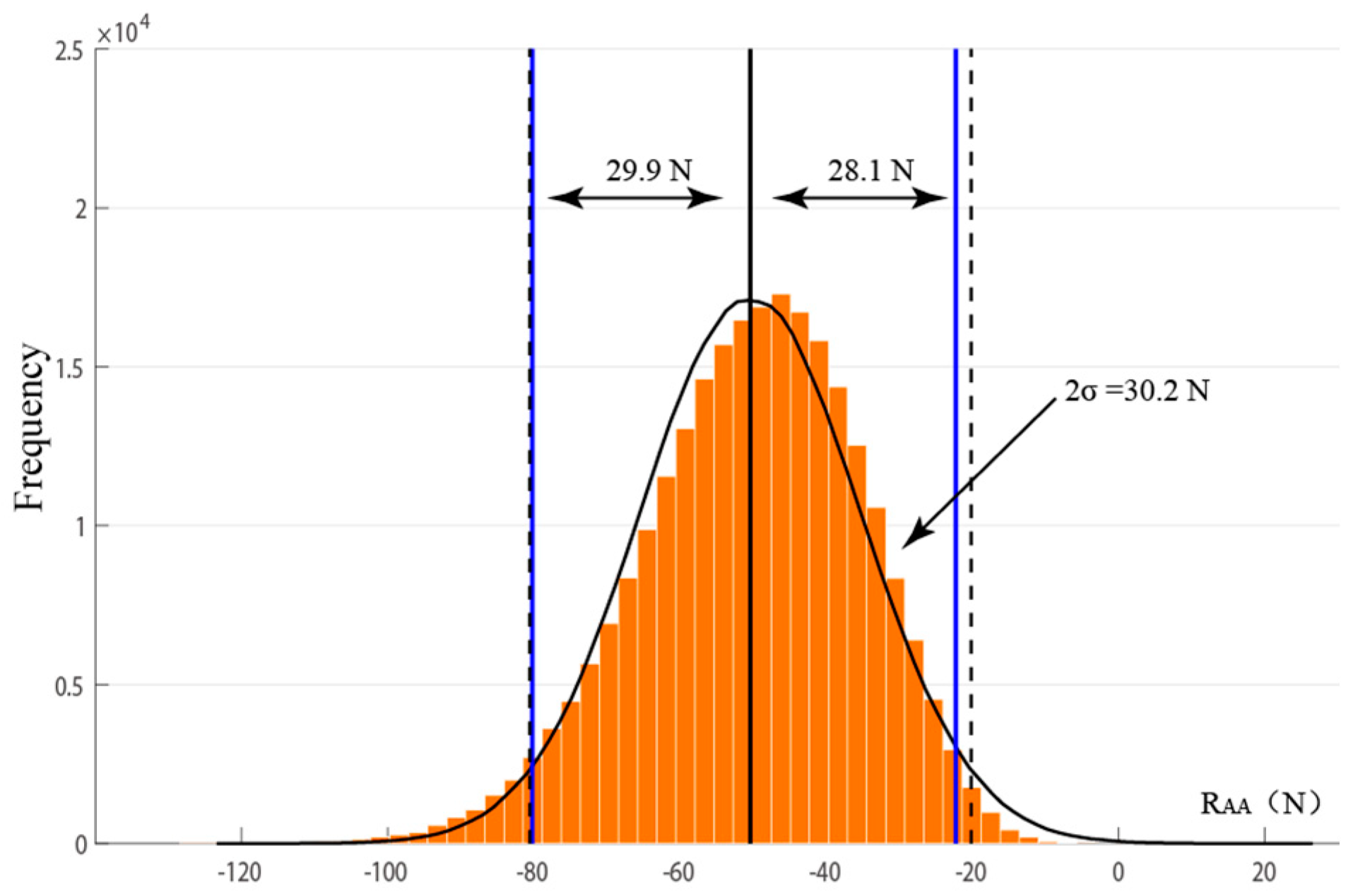
Notably, in order to facilitate calculation of the total uncertainty and the statistics of the data, the distribution function of the wind resistance was approximated to a normal distribution, which is not completely equal to the actual simulation results. For example, the wind resistance distribution of the ship model when the propeller speed is 250 r/min in the second test is shown in Figure 3.

It can be seen from the figure that the probability density function of wind resistance shows a slight asymmetry. In the 95% probability inclusion interval, the distance between the two endpoints and the mean is close. Comparing the frequency distribution histogram with the normal distribution curve using the same mean and standard deviation, it is observed that the figure deviation is small and the inclusion intervals are similar. Therefore, it can be considered that this approximation is reasonable, and the corresponding wind resistance can be expressed as follows:

$$\begin{array}{cc}\hfill R_{AA}=& 44.7 \mathrm{N}\pm 23.2 \mathrm{N}(\mathrm{k}=2)\hfill \\ \hfill =& 44.7 \mathrm{N}\times (1\pm 51.9\%)\hfill \end{array}$$

(6)

3.3.2. Uncertainty of Resistance Increase Due to Wave

In this propulsion test, the sea conditions in the sailing sea area were relatively mild. Based on the real-time measurement results of the wave altimeter, the waves encountered by the ship were high-frequency short waves. In this case, the drag increase in hull motion caused by waves can be ignored, and the additional resistance is mainly caused by the wave reflection of the hull on the waterline. Therefore, in this study, the STWAVE-1 method recommended by the ISO was used to estimate the wave resistance, as shown in the following formula:

$$R_{AWL}=\frac{1}{16}{\rho }_{s}g{H}_{W1/3}^{2}B\sqrt{\frac{B}{L_{BWL}}}$$

(7)

Among them, ρ_S is the sea water density = 1026 kg/m³; g = 9.80 m/s²; H_W1/3 represents the significant wave height of 0.14 m; B is the width of the ship model, which is 4.04 m; and L_BWL is the distance from the bow waterline to 95% of the width of the ship, with a measured value of 2.51 m. The vertical acceleration at the bow measured by the sensor was 0.18 m/s² < 0.05 g = 0.49 m/s², which means the trim and pitch conform to the conditions of the formula. In the wave drag increase correction, only the area of the wave direction angle within the heading angle ± 45 is considered, and if the wave direction is outside this area, the wave resistance increase is not considered. In this experiment, only the wave direction angle of the second group test meets the requirement of correction, thus the wave resistance increase of the first group test was zero.

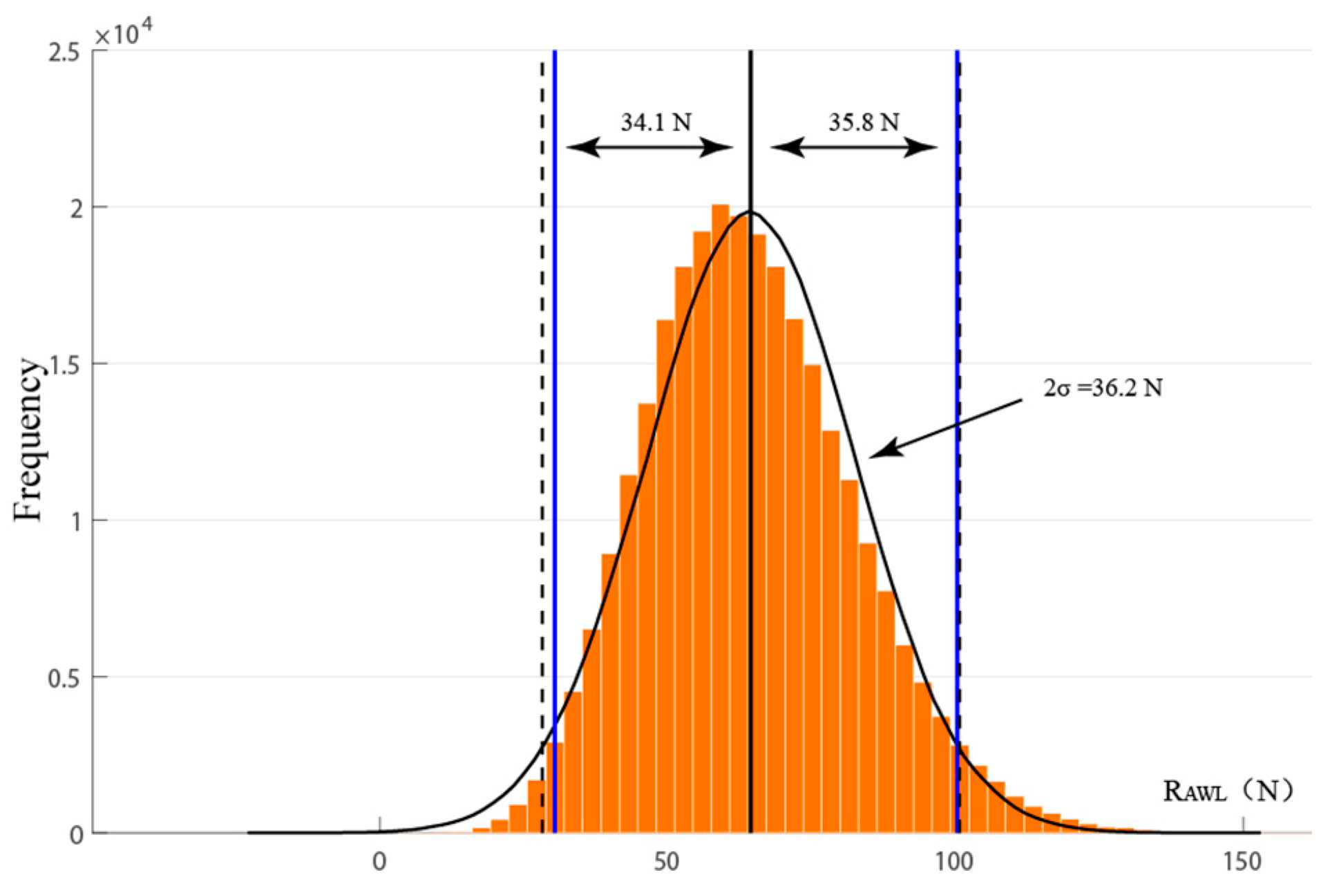
Based on the measurement accuracy of the wave altimeter, the distribution of H_W1/3 in the input is defined as N (0.14, 0.02). Other parameters including the sea water density and the uncertainty of the ship model value were very small, thus negligible here. The frequency distribution histogram of the simulation is shown in Figure 4.

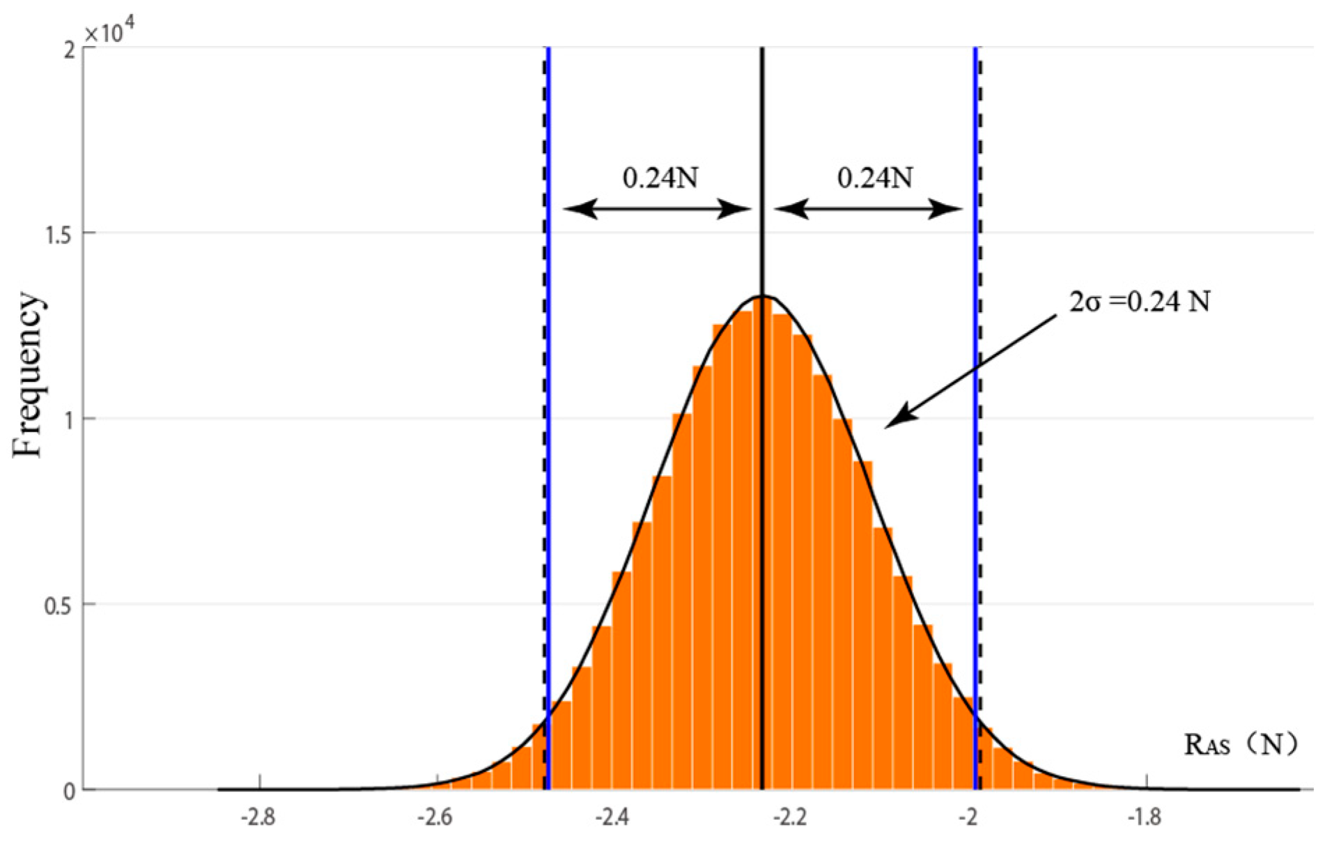
Comparing the histogram with the normal distribution curve, it can be observed that the peak value of the histogram shifts to the left, which may be related to the non-negativity of wave resistance. Considering that their figure deviation is small and the inclusion interval is similar, the distribution function of wave resistance can be approximated as a normal distribution, which can be expressed as follows in 95% confidence probability:

$$\begin{array}{cc}\hfill R_{AWL}=& 64.4 \mathrm{N}\pm 36.2 \mathrm{N}(\mathrm{k}=2)\hfill \\ \hfill =& 64.4 \mathrm{N}\times (1\pm 56.2\%)\hfill \end{array}$$

(8)

3.3.3. Uncertainty of Water

The temperature and density of the water will affect its viscosity, thus affecting the resistance of the ship model. The actual seawater temperature of the test differs from the standard temperature, the prediction and calculation in the propulsion test is usually based on the water temperature of 15 °C, and the viscosity corresponding to 1026 kg/m³ is 1.1892 × 10⁻⁶ m²/s. The sea water temperature in this test was 16.8 °C, thus it requires correction. Since the effect of roughness is not considered, the effect of sea water temperature and density on the resistance can be expressed by the following formula:

$$\begin{array}{l}{R}_{AS}=R_{T0}(\frac{{\rho }_S}{{\rho }_{S0}}-1)-R_F(\frac{C_{F0}}{C_F}-1)\\ R_F=\frac{1}{2}{\rho }_{S}S{V}_S^2{C}_F\\ R_{F0}=\frac{1}{2}{\rho }_{S0}S{V}_S^2{C}_{F0}\\ R_{T0}=\frac{1}{2}{\rho }_{S0}S{V}_S^2{C}_{T0}\end{array}$$

(9)

where C_F is the friction resistance coefficient of the actual water temperature and water density; C_F0 and C_T0 are the friction resistance coefficient and total resistance coefficient of the reference water temperature and water density, respectively; R_F is the friction resistance of actual water temperature and water density; R_F0 and R_T0 are the friction resistance and total resistance of the ship model under reference water temperature and water density, which are calculated from the data obtained from the resistance test; S is wet surface area; V_S is the speed of ship model; and ρ and ρ₀ are the sea water density under actual and reference water temperatures and salt content, respectively. The parameters in the formula were calculated using the ITTC1978 formula, as shown in

Table 5. Water temperature and density correction parameters.

	ρS	CF0	CT0	RT0
200-1	1025.63	0.002598	0.008529	852.21
250-1	1025.63	0.002491	0.007663	1297.47
300-1	1025.63	0.002419	0.007769	1911.02
200-2	1025.63	0.002454	0.004303	880.55
250-2	1025.63	0.002354	0.003759	1314.55
300-2	1025.63	0.002305	0.004152	1911.39

.

Among them, the input water temperature is normally distributed, and the interpolation function of water density and viscosity with respect to temperature change is shown in the following formula:

$$\begin{array}{l}\rho =1028.18-0.0613t-0.0059t^2+0.00003t^3\\ \nu =(1.79952-0.050543t+0.000657t^2)\times {10}^{-6}\end{array}$$

(10)

The tests under various working conditions were simulated respectively, and the expanded uncertainty of resistance affected by water temperature and density of the two groups of tests is shown in

Table 6. Uncertainty of resistance increase due to water (k = 2).

	RAS (N)	U (95%)	U % (95%)
200-1	−2.23	0.24	10.8%
250-1	−3.58	0.39	10.9%
300-1	−5.03	0.55	10.9%
200-2	−3.98	0.43	10.8%
250-2	−6.40	0.69	10.8%
300-2	−8.28	0.89	10.7%

.

It can be seen from the table that the uncertainty of resistance caused by sea water temperature and density increases with the rotational speed, but the relative expansion uncertainty of resistance itself is maintained at roughly 10.8%, which is caused by the measurement accuracy of the thermometer. The value of this uncertainty is large, and it is difficult to reduce from the instrument’s measurement. However, considering that the resistance caused by seawater is small, it has little effect on the total resistance of the ship model.

Figure 5 is the frequency distribution histogram of a working condition, from which we can see that the resistance distribution frequency diagram caused by water temperature and density is consistent with the normal distribution curve.

Furthermore, the distance between the two endpoints and the mean is almost equal in the 95% probability range. Therefore, the related resistance can be expressed as in the following formula:

$$\begin{array}{cc}\hfill R_{AS}=& -2.23 \mathrm{N}\pm 0.24 \mathrm{N} (\mathrm{k}=2)\hfill \\ \hfill =& -2.23 \mathrm{N}\times (1\pm 10.8\%)\hfill \end{array}$$

(11)

3.3.4. Influence of Shallow Water Effect on Speed

The influence of the shallow water effect can be expressed by the following formula (Lackenby shallow-water correction):

$$\frac{\Delta V}{V_S}=0.1242(\frac{A_M}{h^2}-0.05)+1-{(\tanh \frac{gh}{V_S{}^2})}^{1/2}$$

(12)

where A_M is the waterline area of the ship model, h is the water depth of the test area, V_S is the speed of the ship model, and ΔV is the influence of the shallow water effect on the speed. The site of this experiment was an area with a large water depth selected through chart selection as there was no professional instrument. Hence, the influence of shallow water effect was not considered. The uncertainty of shallow water effect is mainly determined by the measurement uncertainty of velocity and water depth.

3.3.5. Influence of Current on Speed

This propulsion test adopted the “MOM” test method recommended by ISO, which assumes that the velocity change of the current flow is parabolic with time. In the test, we carried out two double runs tests under the same rotational speed, that is, four times for each working condition. The speed of the ship model can be expressed as follows:

$$V_S=\frac{V_{G1}+3V_{G2}+3V_{G3}+V_{G4}}{8}$$

(13)

where V_S represents the relative speed of the ship model to the water and V_G1, V_G2, V_G3, and V_G4 are the four ground velocities at each power measured in the test.

The second group of test data was selected to modify the speed of the ship model. All the velocities in this experiment were measured by the Global Positioning System (GPS). Based on its measurement accuracy, the uncertainty of current on velocity was calculated by Taylor formula, as shown in

Table 7. Uncertainty of speed (k = 2).

Run-2	VS (m/s)	U (95%)	U % (95%)
200	1.27	0.02	1.6%
250	1.63	0.02	1.2%
300	2.02	0.02	1.0%

.

It can be seen that as only the systematic error of speed was considered, the expanded uncertainty at each speed is only related to the measurement accuracy of the GPS. Therefore, with increasing ship model speed, the influence of ocean current on speed uncertainty will decrease.

3.4. Uncertainty of Propulsion Test

One purpose of this self-propulsion test was to judge the propulsion performance of the ship. To express the overall hydrodynamic performance of the propulsion system in ship propulsion, the effective power P_E of the ship was compared with the received power P_DB of the propeller, which is called propulsion efficiency η_D:

$${\eta }_D=\frac{P_E}{P_{DB}}=\frac{R_X{V}_s}{2\pi nQ}$$

(14)

R_X = R + ΔR, where resistance R_X is obtained by adding the resistance value measured by the large-scale ship model resistance test performed in the same period to the correction value in the propulsion test. The equation ΔR = R_AA + R_AWL + R_AS expresses the correction and includes changes in resistance caused by wind, wave, and sea water characteristics. Here, we collate the uncertainty calculation results of the previous sections, select the second group of propulsion test data, and summarize the distribution of the parameters in the propulsion coefficient in

Table 8. Distribution of input parameters in propulsion coefficient η_D.

N (r/s)	VS (m/s)	RX (N)	Q (Nm)
N (200, 0.167)/60	N (1.27, 0.01)	N (416.9, 23.51)	N (53.25, 0.083)
N (250, 0.167)/60	N (1.63, 0.01)	N (662.1, 23.57)	N (79.76, 0.083)
N (300, 0.167)/60	N (2.02, 0.01)	N (1000.4, 23.58)	N (117.88, 0.083)

. As this section only evaluates the uncertainty of the propulsion test, the uncertainty of the resistance test is not considered. On the other hand, the resistance value can also be converted from the resistance test data of the towing tank.

The calculation results substituted by the Monte Carlo program are shown in

Table 9. Uncertainty of propulsion coefficient η_D (k = 2).

Run-2	ηD	U (95%)	U % (95%)
200	0.4747	0.05409	11.39
250	0.5168	0.03738	7.23
300	0.5457	0.02629	4.82

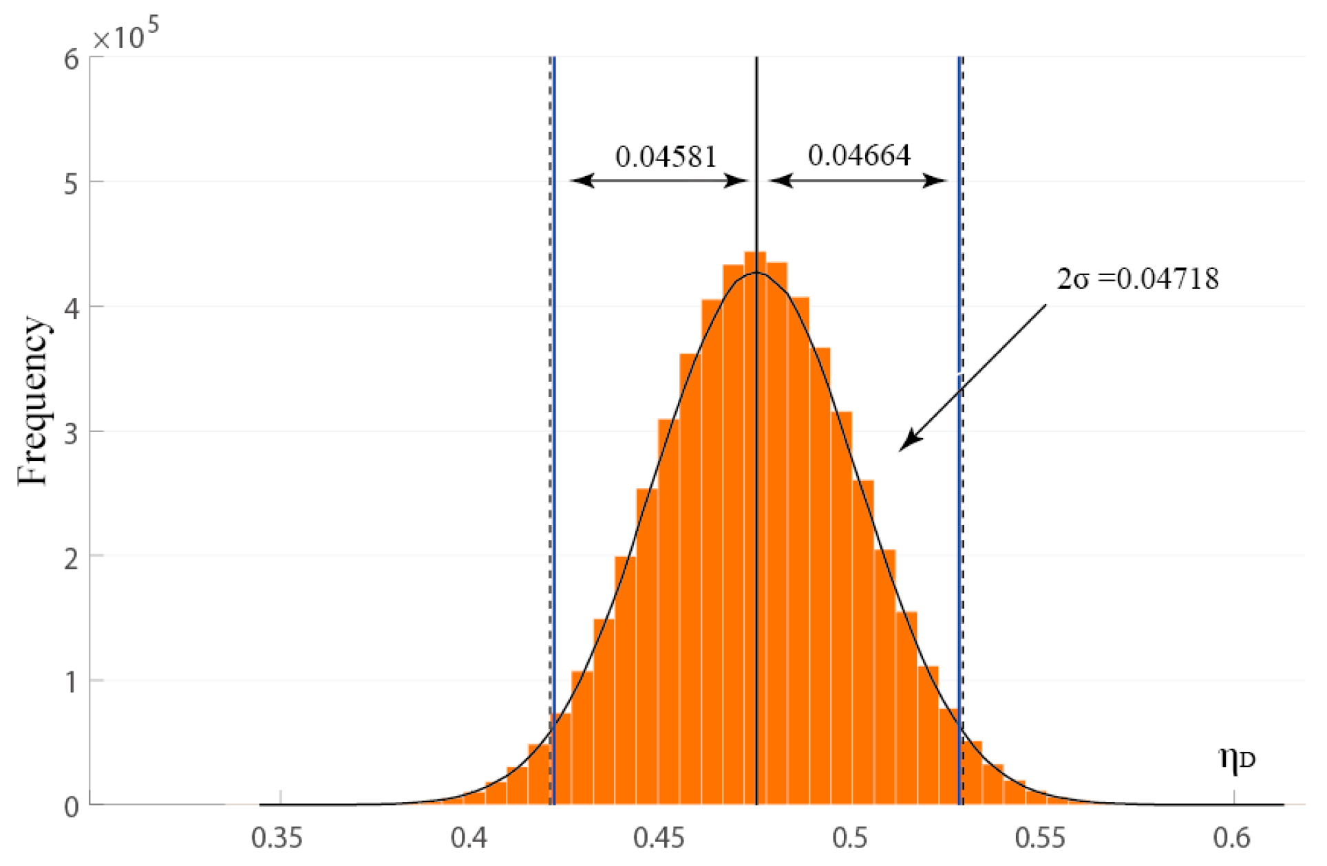
. Figure 6 shows the distribution frequency of the propulsion efficiency at 200 rpm.

It can be seen from the table that when the propeller speed is 200–300 rpm, the uncertainty of propulsion efficiency is between 4.8% and 11.4%, and the uncertainty decreases significantly with the increase in speed. It should be noted that as it is a single test, the uncertainty evaluation of the propulsion test in this study mainly used the evaluation method of type B uncertainty, and other data fluctuations caused by the environment (random error) were not considered, which will lead to the results in the final evaluation being smaller than the actual value.

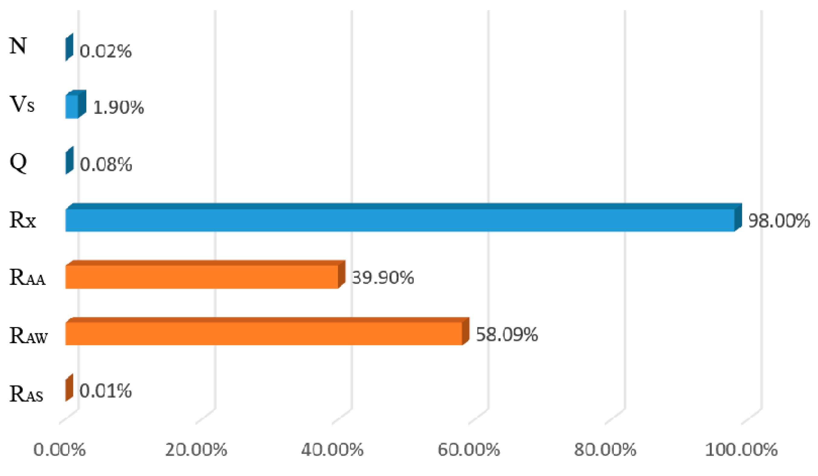
The proportion of uncertainty of each part of the propulsion coefficient is shown in Figure 7. It can be seen from the figure that the effect of resistance correction is the most important as it reached 98%, and the sum of wave resistance and wind resistance accounts for 99% of the uncertainty of resistance correction.

4. Discussion

4.1. Ship Model and Shafting Measurement

The uncertainty related to the conditions of the ship model itself was a small amount in this test. Considering that the interference of these factors to the test was constant throughout the test, their influence was ignored in the evaluation. The Taylor series method was used to analyze the shafting. The uncertainty of shafting conduction has been proven to be very large in a previous ship test [9,16]. However, because the broken-shaft-type self-propulsion in this experiment can directly measure the thrust and torque received by the propeller, the uncertainty of this part was found to be very small. In this case, we can better understand the effects of the environment on the experiment.

4.2. Wind

The relative expanded uncertainty of wind resistance in this propulsion test was very large. On the one hand, it was caused by the measurement accuracy of the instrument. After many simulations, it was found that the selection of measuring instruments with higher accuracy of wind speed improved the test accuracy better. On the other hand, the measurement uncertainty of wind resistance has little relationship with the numerical value of wind resistance itself. This means when the wind resistance of the ship model itself increases, the relative measurement uncertainty can be effectively reduced.

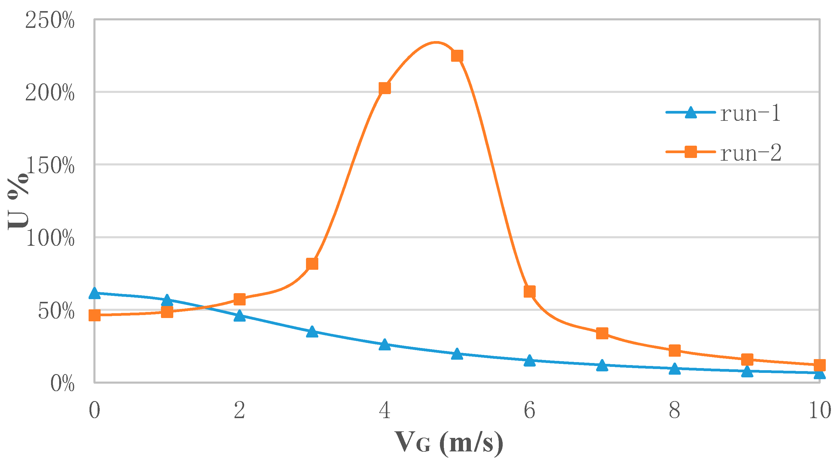
Because the velocity of the ship model has a direct influence on the wind resistance, we numerically simulate the uncertainty of the wind resistance at different speeds. It can be seen from Figure 8 that for the ship model in this test, the relative uncertainty of wind resistance can be controlled below 35% when the speed is above 7 m/s, and the relative uncertainty of wind resistance can be controlled below 25% when the speed of the ship model in this test reaches above 8 m/s. In the case of downwind, when the speed increases to a certain extent, the action direction of the wind resistance will change, and the wind resistance of the ship model will first decrease and then increase with the increase of the speed. Therefore, the uncertainty of the second test will reach a peak when the speed is close to the wind speed.

From the final evaluation of the propulsion coefficient, the wind resistance significantly influenced the test, accounting for about 40%. Therefore, it is important to select the appropriate wind level of the weather and accurately measure the stroke information during the trial. Higher relative velocity will result in greater wind resistance, which is conducive to improving the accuracy of the trial. For this, special attention should be paid to the test under downwind conditions.

4.3. Wave

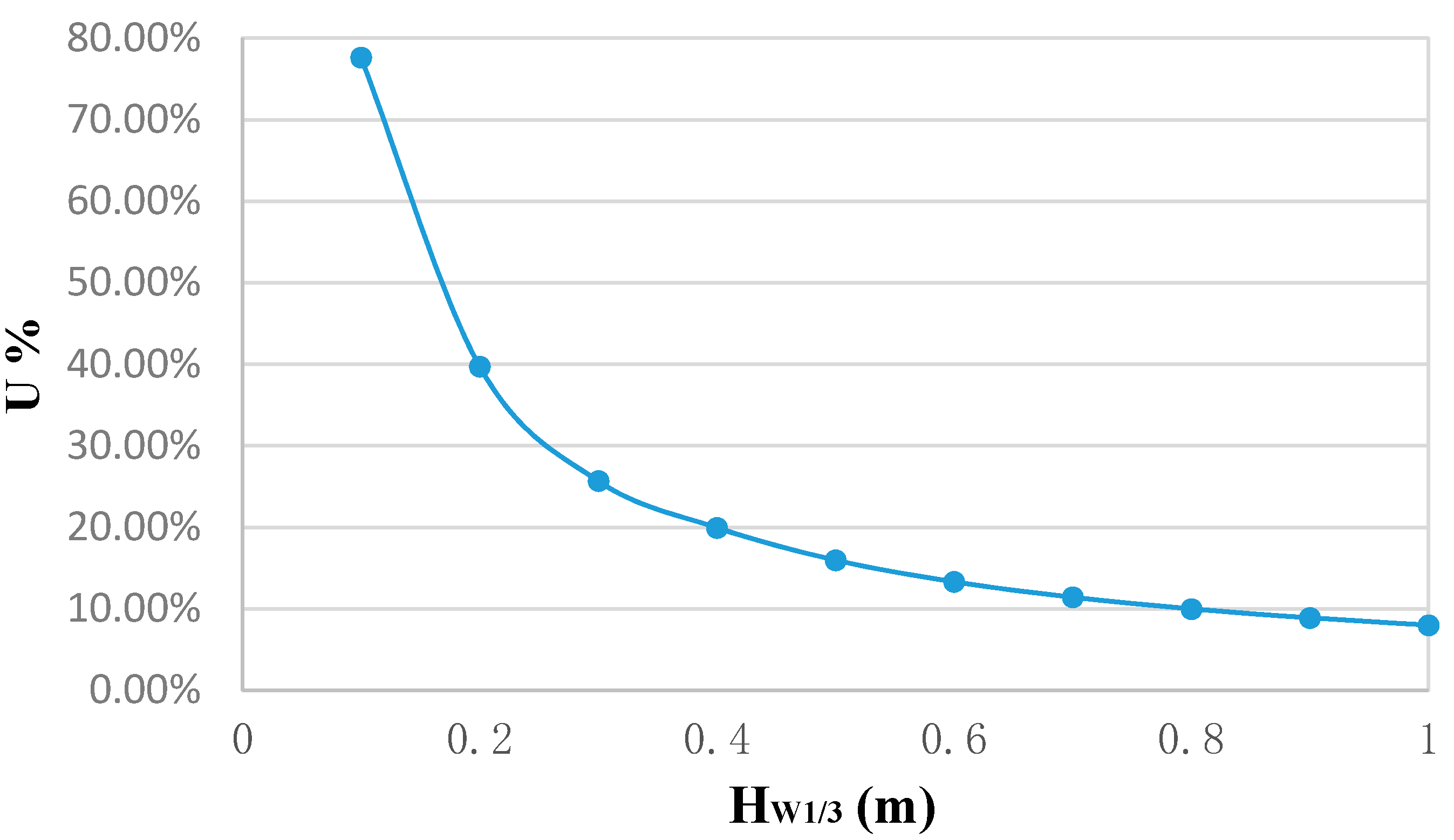
The relative expanded uncertainty of wave resistance was approximately 56.2%, which shows that the measurement uncertainty of wave resistance is very large. Specifically, it was difficult to measure the wave height of 0.14 m with the wave altimeter in this experiment, mainly because the test site was offshore and the sea conditions on the test day were very mild. Through the numerical simulation of the uncertainty of wave resistance under different wave heights, the curve of Figure 9 can be obtained. It can be seen that for the equipment and ship model in this test, the uncertainty decreases significantly when the wave height increases from 0.1 m to 0.3 m.

Therefore, for the ship model test on actual seas, choosing a more significant wave environment is beneficial to improve the measurement accuracy. However, when the wave height reaches a certain level, the promotion will be slow, and the conversion of the actual working conditions, the safety of the test and other factors need to be taken into account. For example, in this experiment, the environment needs to be close to the condition of still water, so the wave height is required. The best way for this case is to improve the measurement accuracy of the instrument (wave altimeter). Through calculation, when the measurement accuracy of wave height is doubled, the uncertainty will be reduced to about half of the original.

In addition, since the STWAVE-1 method only considers the influence of meaningful wave height, which may be different from the actual wave resistance experienced by the ship model, especially in strong sea conditions. Therefore the wave resistance estimation method other than the STWAVE-1 method can be adopted to obtain more accurate results by comprehensively considering wave direction, period and other factors.

In the final evaluation, it was found that wave had the greatest effect on this test, which is consistent with our perception in the actual test process. Owing to the requirements of the propulsion test, it is important to choose a relatively calm test site, although this is difficult. Moreover, when we analyzed the data of the wave altimeter, we found that the actual wave height might be inaccurate. This is not only because its true value is exceedingly small, but also because our data can only represent the wave information of a certain point near the ship model. Therefore, it is necessary to obtain real-time and multi-point wave information in future research.

4.4. Other Parameters

Finally, the uncertainty caused by water temperature and speed is also insignificant, which is mainly caused by the accuracy of the instrument itself. Notably, the data in this study are a demonstration of the entire test process. However, being limited by the number of tests and measurement mechanism, it cannot effectively express the fluctuation of the data in the test process. Hence, the data is insufficient for studying the effect of environmental changes. In other words, although the uncertainty of the current is very small in this study, it does not mean that the impact of the current on the test can be ignored. This is partly because currents are difficult to measure with our equipment and may require testing in somewhat more pronounced environmental conditions. On the other hand, we did not consider the influence of random error in this study, so the influence of current in the test was not fully shown. In fact, during the test on seas, we could feel that the effect of the current on the ship model is significant and variable.

According to the results of the evaluation, the effect of wind and wave is the most important factor in this propulsion test. Thus, it is important to improve the test accuracy of wind speed, direction, and wave measurement instruments. In this experiment, the measurement accuracy of wind direction has much room for improvement, and it is necessary to set up two devices to collect wave direction and water depth, respectively. On the other hand, when the speed of the ship model becomes higher, the relative uncertainty of parameters such as wind resistance and speed will be significantly reduced. Therefore, if the conditions permit, we can consider increasing the speed of the ship model to obtain a higher test accuracy.

It can be seen that even though the uncertainty of the environmental parameters in this experiment is very large, the total uncertainty of the propulsion coefficient is relatively small. This is because the wind and wave conditions selected in this experiment are mild, so the corresponding correction value is relatively small. If the experiment is carried out under the condition of a severe environment, the uncertainty of environmental parameters will be smaller, but the correction value will be larger. Therefore, before the test, the research team should estimate the uncertainty according to the test content and the environment at that time, and adjust the test instrument or working condition according to the initial test data. The improvement measures in this study should be helpful to the measurement of most tests on actual seas.

5. Conclusions

In this study, we mainly used the self-adaption program based on the Monte Carlo method to analyze the uncertainty of a ship model propulsion test on a real sea. By comparing the histogram simulated by the Monte Carlo method with the probability density function curve of the normal distribution, only a little deviation was observed between them. Hence, the uncertainty components of each part can be expressed by the results of an approximate normal distribution. Thus, the influence of the test environment was quantified, and the composition of the total uncertainty was analyzed. From the analysis in this study, it can be concluded that the wind and waves in an environment are the two factors with the greatest influence on the test accuracy.

In the subsequent design process of similar tests on actual seas, the experimenter should focus on these two aspects and select appropriate measuring instruments and an environment according to the test content. In addition, an important research work is to quantify the uncertainty of current, and we believe that its influence cannot be ignored.

Owing to the limitations of instruments and test time, this study did not take into account the impact of data fluctuations in the test process. In fact, parameters such as wind, waves and currents in the marine environment are constantly changing, and it may be inaccurate to replace these values with only a few data points or averages. Therefore, the next goal will be to undertake an in-depth study of the sources of uncertainty in the environment by improving the experimental scheme and analysis methods. Furthermore, uncertainty analysis of relevant towing-tank tests in controlled conditions will also be carried out, so as to reflect the interference factors in the actual environment directly.