Two-Dimensional Numerical Modelling of a Moored Floating Body under Sloping Seabed Conditions

Abstract

A coupled floating body-mooring line model is developed by combining a boundary element model for a two-dimensional floating body and a catenary mooring line model. The boundary element model is formulated in the time domain by a continuous Rankine source, and a reflection potential is introduced to account for the wave reflection due to sloping seabed. This newly developed model is validated by comparisons against available data. Then, dynamic response analyses are performed for the moored body in various seabed conditions. Compared with a flat seabed, a sloping seabed causes unsymmetrical mooring line configuration and generates noticeable effects in the motion responses of the floating body.

1. Introduction

Many types of offshore structures, including floating islands [1], floating shelters [2], floating wind turbines [3], floating wave energy converters [4] and floating offshore fish farms [5], are moored in complicated coastal environments. These structures are exposed to ocean waves, with the possibility of wave reflection and wave shoaling from coastal seabeds. Dynamic responses of these floating bodies are the combined effects of ocean environments and mooring systems. Accurate predictions of dynamic responses are of practical importance for the design and manufacture of these offshore structures.

Compared with that of deep water offshore structures, design and construction of floating structures in coastal environments face unique challenges and the dynamics of these structures could be more complicated because of the seabed effects. Previous researches suggest that shallow waters can excite larger responses of offshore structures under hydrodynamic loading because of the flat seabed effects [6,7,8]. As numerical approaches for flat seabeds are not directly applicable to sloping seabed profiles, refs. [9,10] developed second-body models to account for the sloping seabed effect within the boundary element model frame and found that a sloping seabed significantly influences the cross coupling hydrodynamic coefficients. Refs. [11,12] developed multi-domain approaches that divide the fluid domain into an interior domain of variable water depth and an exterior domain of constant depth. An extra term accounting for the sloping-bottom effects is introduced to correct the incident wave potential so that the sloping seabed condition is satisfied. They found that the sloping seabed significantly affects the body motion response amplitude operator (RAO). Ref. [13] coupled a Rankine source model to the Boussinesq equation, which supplies all relevant information concerning the fluid domain. They reported that the peak frequency of the exciting forces and motion responses are shifted ahead due to the sloping seabed effects. Refs. [14,15] introduced a reflection velocity potential to account for the sloping seabed effect. Numerical results demonstrated that the sloping seabed alters the symmetrical profile of the fluid domain and the coupled effects between different motion modes become important. However, the mooring lines are not considered in these numerical models.

Mooring systems serve as station-keeping devices used to maintain a floating body in acceptable positions. Mooring systems can be categorised based on the restoring mechanisms, weathervaning characteristics and so forth. For a taut-leg mooring, the elastic stiffness due to line stretch is the dominant source of restoring, while for a catenary mooring configuration, the mooring restoring comes primarily from the geometry stiffness of the lines in normal sea states as the floating structure moves within certain offset ranges [16]. As a result of the relatively cheap anchoring costs and convenient offshore installation, the catenary mooring configuration has been extensively applied in various water depths [17,18] and with different component compositions [19]. For instance, Ref. [20] found that proper application of clump weights and buoys can increase the mooring restoring force and floating body capacity, but this will add extra difficulty for practical operation.

Numerical modelling of catenary mooring lines has different levels of fidelity. The quasi-static approach based on the catenary equations does not consider mooring dynamics and facilitates frequency-domain analysis for preliminary design purposes [21]. For deep-water applications, the dynamic mooring line tension becomes more important, and semi-analytical methods accounting for simplified dynamics were also proposed [22]. Later, finite element models [23,24] and lumped-mass models [25] were proposed for time-domain simulations, and these models provide accurate representation of the mooring line dynamics at increased computational costs.

Concerning the modelling of floating body and mooring lines, both uncoupled and coupled analysis have been applied. An uncoupled model essentially ignores the interactions between the floating body and treats a mooring line as a simple massless spring [26,27]. Such an approach benefits from less computational cost but sacrifices result accuracy. In comparison, a coupled model addresses the interaction between the floating body and mooring lines and can be particularly important if accurate mooring responses are needed. For a coupled model, frequency-domain and time-domain panel models have been developed to describe the wave phenomena and wave forces. As shown by [28], both frequency- and time-domain models can be used to deal with nonlinear waves around the floating body, although the latter is less ambiguous for the scattered waves.

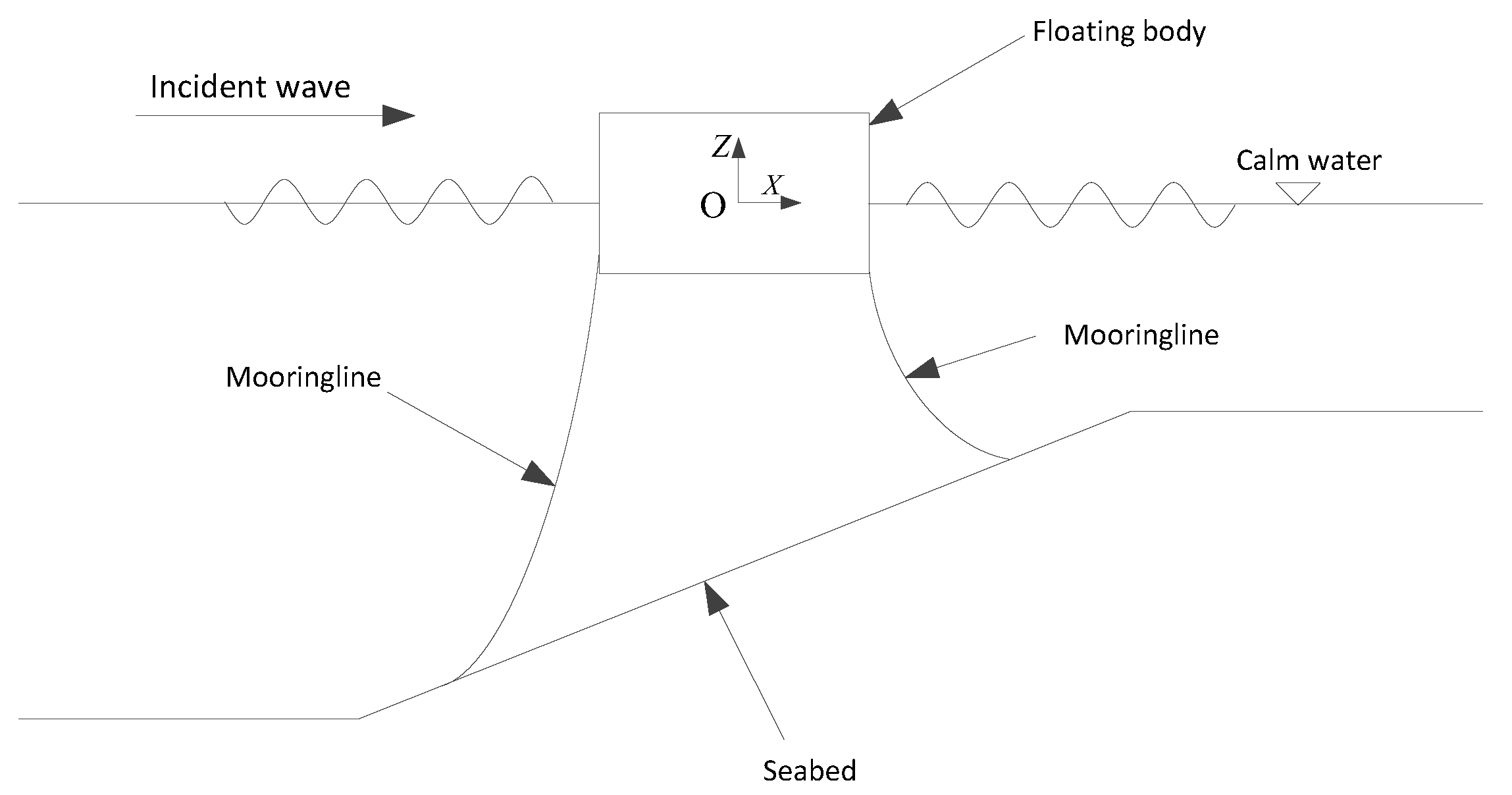
Many offshore renewable energy facilities such as wave energy converters are moored in coastal areas with shallow water. Depending on the site conditions, the mooring lines may lie on a sloping seabed, which will change the fluid dynamics and eventually affect the mooring dynamics and power production performance. To examine the influence of seabed conditions without loss of generality, we only consider a floating body with mooring lines in this work. A simplified catenary model is adopted together with a boundary integral method to develop a time-domain coupled numerical model. The boundary integral model comprises three boundary element equations accounting for wave diffraction, wave radiation and wave reflection, respectively. This coupled model is validated by comparison against published data for the static offset, free decay and regular wave tests. Furthermore, numerical simulations are performed for various seabed profiles and mooring line conditions. The numerical study shows that the sloping seabed significantly changes the fluid domain and mooring line profile and therefore results in noticeable effects on the dynamic responses of the coupled floating body-mooring line system. These effects also vary under different sloping seabed with asymmetrical mooring lines conditions compared with the flat seabed case.

It should be noticed that in real ocean environments, inclined seabeds can lead to formation of vortices of various scales which affect the mooring line mechanism as well as the floating body motion characteristics. The present fluid domain is described by potential flow and flow viscosity is essentially ignored. The investigation of vortices on the mooring line and body motion is out of the scope of the present study.

2. Problem Formulation

2.1. Coupled Floating Body-Mooring Line Model

For a free-floating body moored in coastal environment, the position and velocity of the floating body vary at each time step and mooring line supplies restoring force to keep the body in acceptable positions. The coupled motion equation for a floating body with mooring lines can be expressed in the form:

$$\sum _{j=1}^3{M}_{ij}{\ddot{X}}_j\left(t\right)=F_i^{wave}\left(t\right)+F_i^{mooring}\left(t\right)+F_i^{static}\left(t\right)(i=1,2,3),$$

(1)

where $M_{ij}$ and ${\ddot{X}}_j\left(t\right)$ respectively denote the body mass matrix and body acceleration. $F_i^{wave}\left(t\right)$, $F_i^{mooring}\left(t\right)$ and $F_i^{static}\left(t\right)$ denote wave force, mooring line force and hydrostatic force, respectively. $F_i^{wave}\left(t\right)$ consists of wave radiation and wave diffraction forces. $i,j=1,2,3$ stand for surge, heave and pitch motion, respectively. In the present study, the coupling effects between different motion modes are ignored for simplification and therefore Equation (1) can be further expressed as:

$$M_{11}{\ddot{X}}_1\left(t\right)=F_1^{wave}\left(t\right)+F_1^{mooring}\left(t\right)+F_1^{static}\left(t\right),$$

(2)

$$M_{22}{\ddot{X}}_2\left(t\right)=F_2^{wave}\left(t\right)+F_2^{mooring}\left(t\right)+F_2^{static}\left(t\right),$$

(3)

$$M_{33}{\ddot{X}}_3\left(t\right)=F_3^{wave}\left(t\right)+F_3^{mooring}\left(t\right)+F_3^{static}\left(t\right).$$

(4)

2.2. Catenary Mooring Line Model

The boundary conditions applied on the mooring lines are the constraints at the two ends of the line: the upper end is attached to the floating platform and is forced to move with the platform, and the lower end is connected to an anchor point at seafloor. For a catenary mooring configuration, a portion of catenary line should lie on the seabed to avoid large vertical forces on the anchors.

The following key assumptions are applied during the analysis of a catenary model: (1) The mooring line moves very slowly such that the drag forces and inertial forces are negligible. (2) The environmental loads on the mooring line are insignificant and can be excluded in the model. (3) The mooring line is inelastic. (4) The anchor point does not move in any directions. (5) The mooring line is lying on a horizontal seabed. In the present study, the sloping seabed inclination is small and the sloping seabed effects for the mooring line mechanism are therefore ignored. This simplification justifies the application of catenary mooring line model to horizontal seabed profiles. For a catenary mooring line with length L, under its own weight of W per unit length in water, the governing equations can be analytically expressed as [29] (pp. 258–263):

$$L-L_z{(1+2\frac{T_x}{L_{z}W})}^{\frac{1}{2}}+\frac{T_x}{W}{cosh}^{-1}(1+\frac{L_{z}W}{T_x})-L_x=0,$$

(5)

$$T_z=W{(L_x^2+2L_{x}W)}^{\frac{1}{2}},$$

(6)

where $L_x$ and $L_z$ are the horizontal and vertical distances between the two ends points of a mooring line, respectively. $T_x$ and $T_z$ are the horizontal and vertical tension, respectively. A sketch of the catenary mooring line model is presented in Figure 1.

At an initial time $t=0$, a mooring line pretension $T_{pre}$ is applied to keep the floating body at a static equilibrium position. At each time step, an iterative scheme is applied to calculate the mooring line forces based on Equation (5). This force is used as the exciting mooring line force on the right-hand side of Equation (1) and then the equation is solved using a fourth-order Runge-Kutta method. The floating body displacement works as boundary conditions for the upper end of mooring line. Then, at the next time step, Equation (5) is solved again to start another loop until the end of the numerical simulation.

2.3. Fluid Domain Formulation

2.3.1. Fluid Motion Equations

Figure 2 illustrates a coordinate frame $OXZ$ with its origin O at the centre of a two-dimensional floating body-mooring line system in a fluid domain of finite water depth. The fluid domain $\Omega$ is bounded by a free surface $S_f$, a body surface $S_b$, a seabed surface $S_0$ and an enclosing surface at infinity, $S_{\infty }$. The fluid flow is assumed to be irrotational and can be described by the velocity potential, $\varphi$, which satisfies the Laplace equation as follows,

$$\frac{{\partial }^2\varphi }{\partial x^2}+\frac{{\partial }^2\varphi }{\partial z^2}=0\mathrm{in} \mathrm{the} \mathrm{fluid} \mathrm{domain} \Omega .$$

(7)

Based on linear theory, the velocity potential $\varphi$ can be expressed as:

$$\varphi (x,z,t)={\varphi }_I(x,z,t)+{\varphi }_D(x,z,t)+{\varphi }_R(x,z,t)+{\varphi }_{re}(x,z,t),$$

(8)

where ${\varphi }_I$, ${\varphi }_D$, ${\varphi }_R$ and ${\varphi }_{re}$ denote the incident wave potential, diffraction potential, radiation potential and reflection potential, respectively. The radiation potential is used to describe the velocity potential generated by floating body motions. For two-dimensional problems, a floating body can undergo surge, heave and pitch motions. For different degrees of freedom, the radiation potential essentially has different values.

2.3.2. Diffraction, Radiation and Reflection Potential Problems

The velocity potentials ${\varphi }_I$, ${\varphi }_D$, ${\varphi }_R$ and ${\varphi }_{re}$ satisfy the Laplace equation, and ${\varphi }_D$, ${\varphi }_R$ and ${\varphi }_{re}$ can be investigated by formulating the boundary integral equations accordingly based on the work of [8,14,30]. The diffraction potential, ${\varphi }_D(x,z,t)$, describes the fluid field potential generated by the incoming wave within the seabed environment. For an incoming progressive linear wave with a wave amplitude, A, in a finite water depth, h, the velocity potential, ${\varphi }_I$ and the wave elevation, ${\eta }_I$, can be expressed as

$${\varphi }_I=\frac{gA}{\omega }\frac{coshk(z+h)}{coshkh}sin(kx-\omega t),$$

(9)

$${\eta }_I=Acos(kx-\omega t),$$

(10)

where g, k and $\omega$ denote the gravitational acceleration, wave number and wave frequency, respectively.

As no fluid penetrates the rigid body and seabed surfaces, the boundary conditions applied to the body and flat seabed are:

$$\frac{\partial {\varphi }_D}{\partial {\mathbf{n}}_b}=-\frac{\partial {\varphi }_I}{\partial {\mathbf{n}}_b}\mathrm{on} S_b,$$

(11)

$$\frac{\partial {\varphi }_D}{\partial {\mathbf{n}}_{\mathbf{0}}}=0\mathrm{on} S_0,$$

(12)

where ${\mathbf{n}}_b$ and ${\mathbf{n}}_0$ denote normal vector on body surface and seabed surface, respectively.

The linearised kinematic condition and the dynamic free surface boundary condition are given as

$$\frac{\partial {\varphi }_D}{\partial z}-\frac{\partial {\eta }_D}{\partial t}=0\mathrm{on} S_f,$$

(13)

$$\frac{\partial {\varphi }_D}{\partial t}+g{\eta }_D=0\mathrm{on} S_f,$$

(14)

where ${\eta }_D$ refers to the wave elevation caused by wave diffraction. The body boundary condition (Equation (11)), seabed condition (Equation (12)) and free surface boundary conditions (Equations (13) and (14)) create a closed boundary value formulation to the diffraction potential problem.

The radiation potential, ${\varphi }_R(x,z,t)$, accounts for the fluid field potential caused by body motions in the fluid domain. Nonpermeable boundary condition is applied to the body and seabed conditions. The free surface boundary condition is simplified as a linear form:

$$\frac{\partial {\varphi }_R}{\partial {\mathbf{n}}_b}={\mathbf{v}}_b·{\mathbf{n}}_b\mathrm{on} S_b,$$

(15)

$$\frac{\partial {\varphi }_R}{\partial {\mathbf{n}}_0}=0\mathrm{on} S_0,$$

(16)

$$\frac{\partial {\varphi }_R}{\partial z}-\frac{\partial {\eta }_R}{\partial t}=0\mathrm{on} S_f,$$

(17)

$$\frac{\partial {\varphi }_R}{\partial t}+g{\eta }_R=0\mathrm{on} S_f,$$

(18)

where ${\mathbf{v}}_b$ denotes the body motion velocity. For a floating body experiencing forced oscillatory motion with an amplitude a, the body motion velocity ${\mathbf{v}}_b$ can be described as:

$${\mathbf{v}}_b=(a\omega cos\omega t,0)\mathrm{for} \mathrm{surge} \mathrm{motion},$$

(19)

and

$${\mathbf{v}}_b=(0,a\omega cos\omega t)\mathrm{for} \mathrm{heave} \mathrm{motion}.$$

(20)

In the proposed model, the free surface is divided into inner and outer domains, which are discussed in the next section. In the outer domain, the source panels are arranged in an exponentially increasing manner. Using this distribution method, a very large free surface can be covered by the source panels and therefore the generated waves can move towards the far field in this enlarged computational domain before the end of numerical simulation. The radiation condition is satisfied without applying any artificial damping on the free surface.

The sloping seabed provides a source of wave reflections into the fluid domain. In this investigation, the wave reflection potential, ${\varphi }_{re}$, is introduced to satisfy the Laplace Equation (7) whose solution is determined by solving the following boundary value equations

$$\frac{\partial {\varphi }_{re}}{\partial {\mathbf{n}}_b}=0\mathrm{on} S_b,$$

(21)

$$\frac{\partial {\varphi }_{re}}{\partial z}-\frac{\partial {\eta }_{re}}{\partial t}=0\mathrm{on} S_f,$$

(22)

$$\frac{\partial {\varphi }_{re}}{\partial t}+g{\eta }_{re}=0\mathrm{on} S_f,$$

(23)

$$\frac{\partial {\varphi }_{re}}{\partial {\mathbf{n}}_0}=-\frac{\partial {\varphi }_I}{\partial {\mathbf{n}}_0}\mathrm{on} S_0,z=h\left(x\right).$$

(24)

Notice that this boundary value equation is analogous to the solution of the wave diffraction potential. In this regard, the potential $\varphi$ can be considered as the potential caused by the interaction of the floating body (the first body) and the sloping seabed (the second body). Equation (24) describes the sloping seabed boundary condition whereas, in Equation (12), the constant water depth refers to the deeper water depth on the left hand side of the sloping seabed. If the seabed is completely flat, the reflection potential ${\varphi }_{re}$ disappears. In this scenario, the reflected wave moves towards the left hand side of the fluid domain and travels into the far field. As the proposed free surface source distribution method covers a very large free surface area on both sides of the body, the reflected wave will not reflect backwards the fluid domain.

2.3.3. Numerical Discretisation of Velocity Potential ${\varphi }_D$, ${\varphi }_R$ and ${\varphi }_{re}$

The velocity potential $\varphi$ can be expressed as a boundary integral of Rankine sources continuously distributed on the fluid boundary surface $S=S_b\cup S_f\cup S_0$ as

$$\varphi ({\mathbf{x}}^{\prime },t)={\int }_{S_b}{\sigma }^{b}ln|{\mathbf{x}}^{\prime }-\mathbf{x}|d{s}_{\mathbf{x}}+{\int }_{S_f}{\sigma }^{f}ln|{\mathbf{x}}^{\prime }-\mathbf{x}|d{s}_{\mathbf{x}}+{\int }_{S_0}{\sigma }^{0}ln|{\mathbf{x}}^{\prime }-\mathbf{x}|d{s}_{\mathbf{x}},$$

(25)

where ${\mathbf{x}}^{\prime }=(x^{\prime },z^{\prime })$ and $\mathbf{x}=(x,z)$ are the control point and the source point, respectively. In this paper, a continuous panel is applied to replace the isolated source point method. The control point is the point where the boundary condition is satisfied and it is located in the middle of a continuous panel. The source point is the end point defining the continuous panel. Each continuous panel has two source points and one control point. ${\sigma }^b$, ${\sigma }^f$ and ${\sigma }^0$ denote the source strength of the body, free surface and seabed, respectively.

Let the integral domain boundary surfaces $S_b$, $S_f$ and $S_0$ be approximated as the sums of $N_b$, $N_f$ and $N_0$ panels, respectively such that $S_b={\cup }_{i=1}^{N_b}{S}_i^b$, $S_f={\cup }_{j=1}^{N_f}{S}_j^f$ and $S_0={\cup }_{k=1}^{N_0}{S}_k^0$. Let ${{\mathbf{x}}^{\prime }}_i^b\in S_b$, ${{\mathbf{x}}^{\prime }}_j^f\in S_f$ and ${{\mathbf{x}}^{\prime }}_k^0\in S_0$ be the control points for $i=1,\dots ,N^b$, $j=1,\dots ,N^f$ and $k=1,\dots ,N^0$. The discretised form of the boundary integral (Equation (25)) describing the diffraction problem is given as:

$$\begin{array}{cc}\hfill \frac{\partial {\varphi }_D\left({{\mathbf{x}}^{\prime }}_i^b\right)}{\partial {\mathbf{n}}_b}& =\sum _{i=1}^{N^b}{\sigma }_i^b\frac{\partial }{\partial {\mathbf{n}}_b^i}{\int }_{S_i^b}ln|{{\mathbf{x}}^{\prime }}_i^b-{\mathbf{x}}_i|d{s}_{\mathbf{x}}\hfill \\ \hfill & +\sum _{j=1}^{N^f}{\sigma }_j^f\frac{\partial }{\partial {\mathbf{n}}_b^i}{\int }_{S_j^f}ln|{{\mathbf{x}}^{\prime }}_i^b-{\mathbf{x}}_j|d{s}_{\mathbf{x}}+\sum _{k=1}^{N^0}{\sigma }_k^0\frac{\partial }{\partial {\mathbf{n}}_b^i}{\int }_{S_k^0}ln|{{\mathbf{x}}^{\prime }}_i^b-{\mathbf{x}}_k|d{s}_{\mathbf{x}},\hfill \end{array}$$

(26)

$$\begin{array}{cc}\hfill \frac{\partial {\varphi }_D\left({{\mathbf{x}}^{\prime }}_j^f\right)}{\partial {\mathbf{n}}_f}& =\sum _{i=1}^{N^b}{\sigma }_i^b\frac{\partial }{\partial {\mathbf{n}}_f^j}{\int }_{S_i^b}ln|{{\mathbf{x}}^{\prime }}_j^f-{\mathbf{x}}_i|d{s}_{\mathbf{x}}\hfill \\ \hfill & +\sum _{j=1}^{N^f}{\sigma }_j^f\frac{\partial }{\partial {\mathbf{n}}_f^j}{\int }_{S_j^f}ln|{{\mathbf{x}}^{\prime }}_j^f-{\mathbf{x}}_j|d{s}_{\mathbf{x}}+\sum _{k=1}^{N^0}{\sigma }_k^0\frac{\partial }{\partial {\mathbf{n}}_f^j}{\int }_{S_k^0}ln|{{\mathbf{x}}^{\prime }}_j^f-{\mathbf{x}}_k|d{s}_{\mathbf{x}},\hfill \end{array}$$

(27)

$$\begin{array}{cc}\hfill \frac{\partial {\varphi }_D\left({{\mathbf{x}}^{\prime }}_k^0\right)}{\partial {\mathbf{n}}_0}& =\sum _{i=1}^{N^b}{\sigma }_i^b\frac{\partial }{\partial {\mathbf{n}}_0^k}{\int }_{S_i^b}ln|{{\mathbf{x}}^{\prime }}_k^0-{\mathbf{x}}_i|d{s}_{\mathbf{x}}\hfill \\ \hfill & +\sum _{j=1}^{N^f}{\sigma }_j^f\frac{\partial }{\partial {\mathbf{n}}_0^k}{\int }_{S_j^f}ln|{{\mathbf{x}}^{\prime }}_k^0-{\mathbf{x}}_j|d{s}_{\mathbf{x}}+\sum _{k=1}^{N^0}{\sigma }_k^0\frac{\partial }{\partial {\mathbf{n}}_0^k}{\int }_{S_k^0}ln|{{\mathbf{x}}^{\prime }}_k^0-{\mathbf{x}}_k|d{s}_{\mathbf{x}}.\hfill \end{array}$$

(28)

At any time step t during the numerical simulation, the body and the seabed boundary conditions are described by their boundary value equations. The free surface boundary conditions for diffraction potential ${\varphi }_D$, radiation potential ${\varphi }_R$ and reflection potential ${\varphi }_{re}$ are all updated by a 3rd-order Adams-Bashforth scheme. The time interval $\Delta t=T_0/100$ is applied in the numerical simulations. Here, $T_0$ is the wave period.

A matrix equation is formulated by discretising Equations (26)–(28). At each time step t, the boundary conditions work as inputs to this matrix equation and the source strength ${\sigma }_i^b$, ${\sigma }_j^f$ and ${\sigma }_k^0$ are the solutions of this equation. Once the source strengths are obtained, the velocity potential $\varphi$ can be investigated based on Equation (25).

The discretisation for the wave radiation, ${\varphi }_R$, and the reflection potential, ${\varphi }_{re}$, is exactly the same as that for the diffraction potential, ${\varphi }_D$ and is therefore omitted herein. Calculation of the Rankine source $lnr$ integral in the boundary integral equations is computationally expensive. In this study, a continuous Rankine source panel integral is developed instead of an isolated Rankine source approximation to reduce numerical errors and increase numerical efficiency.

Note that, physically, the free surface, $S_f$, is of infinite size and the integration over this infinite dimension is not possible by numerical techniques. For this reason, the computational domain is truncated in the numerical simulations and the far-field boundary condition is satisfied on this truncated free surface. In the present study, the Rankine source panels are distributed in an exponential manner, allowing for the coverage of a very large area of free surface. The numerical computations are completed before the incident wave and reflected wave reaches the truncated boundary.

2.3.4. Boundary Panel Distribution

In the present study, the sloping seabed $z=h\left(x\right)$ is described mathematically as:

$$h\left(x\right)=\left\{\begin{array}{cc}-H-\frac{L_v}{2}\hfill & x<-\frac{L_h}{2}\hfill \\ -H+xtan\theta \hfill & -\frac{L_h}{2}\le x\le \frac{L_h}{2}\hfill \\ -H+\frac{L_v}{2}\hfill & x>\frac{L_h}{2}\hfill \end{array}\right.$$

(29)

where H is the mean water depth and $\theta$ denotes the sloping seabed angle which is defined as:

$$\theta =arctan\left(\frac{L_h}{L_v}\right),$$

(30)

where $L_h$ and $L_v$ are the projected length of the slope seabed in horizontal and vertical directions, respectively. Figure 3 illustrates the definitions of these parameters in the coupled floating body-mooring line problem under investigation. The sloping seabed is divided into three regions, $h_1$, $h_2\left(x\right)$ and $h_3$. The constants $h_1$ and $h_3$ correspond to the constant depth flat portions on the left and right hand sides of the sloping seabed whereas the variable $h_2\left(x\right)$ represents the depth of water in the sloping region.

Both the free surface and seabed surface are divided into inner and outer domains. To approximate the inner domain, the source panel distribution method discussed by [8] is adopted here. A parameter $\gamma =1+tan\theta$ is introduced to deal with this asymmetric characteristic of the surface. For free surface and flat seabed, the angle $\theta =0$ and therefore $\gamma =1$. On the right side of $S_0$, starting from $x=0$, the horizontal distances between neighbouring control points are expressed as:

$$|{{\mathbf{x}}^{\prime }}_k^0-{{\mathbf{x}}^{\prime }}_{k-1}^0|=\frac{L_b{\alpha }_k}{\gamma {\omega }^2}\mathrm{in} \mathrm{the} \mathrm{inner} \mathrm{domain},$$

(31)

$$|{{\mathbf{x}}^{\prime }}_k^0-{{\mathbf{x}}^{\prime }}_{k-1}^0|=\frac{L_b{\alpha }_k}{\gamma {\omega }^2}{1.05}^{k(k-1)/2}\mathrm{in} \mathrm{the} \mathrm{outer} \mathrm{domain},$$

(32)

and on the left hand side of $S_0$:

$$|{{\mathbf{x}}^{\prime }}_k^0-{{\mathbf{x}}^{\prime }}_{k-1}^0|=\frac{\gamma L_b{\alpha }_k}{{\omega }^2}\mathrm{in} \mathrm{the} \mathrm{inner} \mathrm{domain},$$

(33)

$$|{{\mathbf{x}}^{\prime }}_k^0-{{\mathbf{x}}^{\prime }}_{k-1}^0|=\frac{\gamma L_b{\alpha }_k}{{\omega }^2}{1.05}^{k(k-1)/2}\mathrm{in} \mathrm{the} \mathrm{outer} \mathrm{domain},$$

(34)

where $L_b$ is the body surface panel length. The parameters ${\alpha }_k$ define the separation distances and are decided according to the method discussed by [8]. In the outer domain the distances between the centres of neighbouring source panels are displaced in an exponentially increasing manner as aforementioned.

3. Model Validation

In order to validate the proposed coupled floating body-mooring line model, numerical simulations are performed for the static offset test, the free decay test without mooring line, the free decay test with mooring line and the regular wave simulation. All numerical simulations are conducted in the time domain and converted into the frequency domain for direct comparison against available published data.

3.1. Static Offset Test

The stiffness characteristics of catenary mooring lines are investigated preliminarily by the static offset tests. For a mooring line with a length of L = 100 m and a unit weight of W = 828 N/m, moored in water depth h = 25 m, Figure 4 shows the comparison of this mooring line stiffness curves with respect to horizontal force $T_x$ $\left(a\right)$ and vertical force $T_z$ $\left(b\right)$ between the proposed numerical method and [29] (pp. 258–263). Results from the proposed method show excellent agreement with those of [29]. It is noticed that both the horizontal force $T_x$ and vertical force $T_z$ demonstrate nonlinear characteristics as the mooring line horizontal distance $L_x$ increases and this phenomenon is also called nonlinear “hardening“ behaviour by [26].

3.2. Free Decay Test

The free decay test works as a measurement to determine the natural period T and the damping ratio $\beta$ of the system. In the free decay test, the floating system was offset an initial displacement and allowed to damp out until reaching the equilibrium position. A heave decay test was performed for a semi-circular cylinder with radius 10 m excluding mooring line as a preliminary study. Figure 5 shows comparison of the heave decay test for the semi-circular cylinder between the proposed method, the [31] numerical simulation and the [32] experiment. As shown, the proposed model yields a good agreement compared with the numerical prediction of [31] and experimental data of [32]. The natural period for this cylinder in heave motion is 7.18 s.

Numerical simulations are further performed for the semi-circular cylinder with different mooring line stiffness $K_i$. The mooring line system stiffness $K_i$ is defined as:

$$K_i=\frac{F_i^{mooring}}{X_i}.$$

(35)

where $X_i$ denotes the body offset and is corresponding to the body displacement in Equation (1). Figure 6 shows the surge decay test for the cylinder with mooring line stiffness $K_1=90,000$ N/m, $135,000$ N/m, $180,000$ N/m and $225,000$ N/m, respectively. It is noticed that the decay period and motion amplitude decrease as stiffness $K_i$ increases. The coupled system free decay period can be analytically evaluated by the following equation of [33] (pp. 275–278):

$$T=2\pi /(1-{\beta }^2)/\sqrt{K/(M+a)},$$

(36)

with

$$\beta =\frac{b}{2\sqrt{(M+a)K}},$$

(37)

where subscripts are omitted for simple notation. The body added mass a and damping b can be obtained from the work of [8].

Table 1. Comparison of surge decay period T between Patel (1989) analytical method and proposed numerical method data for mooring line stiffness $K_1=90,000$ N/m, $135,000$ N/m, $180,000$ N/m and $225,000$ N/m, respectively.

Surge Decay Period T
Stiffness $K_1$ (N/m)	Patel (1989) analytical method	Proposed numerical method	Error
90,000	12.77	13.05	2.1%
135,000	10.80	10.65	1.4%
180,000	9.35	9.15	2.0%
225,000	7.15	7.30	2.1%

shows a comparison of the surge decay period T between the analytical method by [33] and the proposed numerical method for the mooring line stiffness of $K_1=90,000$ N/m, $135,000$ N/m, $180,000$ N/m and $225,000$ N/m, respectively. It is observed that the proposed method agrees well with the analytical expression of [33]. The natural period of this floating body-mooring system is around $10$ s. Therefore, the wave frequencies dominate the system responses and low-frequency responses are expected to be small.

3.3. Regular Wave Simulation

Numerical simulations are further carried out for the floating body-mooring system subject to regular waves. As a preliminary study, numerical simulations are conducted for a rectangular cylinder with breadth B = 0.30 m and draft $d=0.20$ m, floating in water depth h = 0.40 m without mooring lines attached. Figure 7 shows a comparison of the time records of surge motion $X_1\left(t\right)$ $\left(a\right)$ and heave motion $X_2\left(t\right)$ $\left(b\right)$ between the proposed method, the experimental data by [34] and the numerical data by [35]. The floating rectangular cylinder is subject to a regular wave with wave period $T_0=1.2$ s and wave amplitude $A=0.02$ m. It is shown that the proposed model results agree favourably well with the model test data of [34] and the numerical prediction of [35]. This floating body is moored by two symmetrical mooring lines, with $L=1.6$ m and a weight of $W=39.2$ N/m in water. Figure 8 demonstrates the comparison of time records of surge motion $X_1\left(t\right)$ $\left(a\right)$ and heave motion $X_2\left(t\right)$ $\left(b\right)$ between proposed method results and [35] numerical data for the rectangular cylinder with the mooring effect included. The numerical data of [35] is shifted with $T=0$ as the starting time for better comparison. It is noticed that the proposed model data agrees reasonably well with the data of [35] for both surge and heave motions. The discrepancy can be explained by the fact that the viscous effects are included in the work of [35] but excluded in the present model.

4. Case Study

For a floating body moored in coastal areas, if the mooring line anchors are located in different water depths, then the mooring line profiles are not symmetrical. The asymmetry of seabed and mooring line profiles significantly affects fluid domain and hence the body response characteristics. By comparing the asymmetrical seabed and moorings with the flat seabed and symmetrical mooring lines, this section investigates the floating body response characteristics in sloping seabed and asymmetrical mooring lines conditions.

A rectangular cylinder with breadth B = 20 m and draft d = 10 m is selected as the floating body. Such a body size is typical of floating bodies in ocean and offshore engineering. An average water depth of H = 200 m is considered for the first numerical case. Two types of seabed and mooring line configurations are used in the numerical simulations. The first type is a flat seabed with two identical mooring lines, and the second one is a sloping seabed with two different mooring line arrangement. 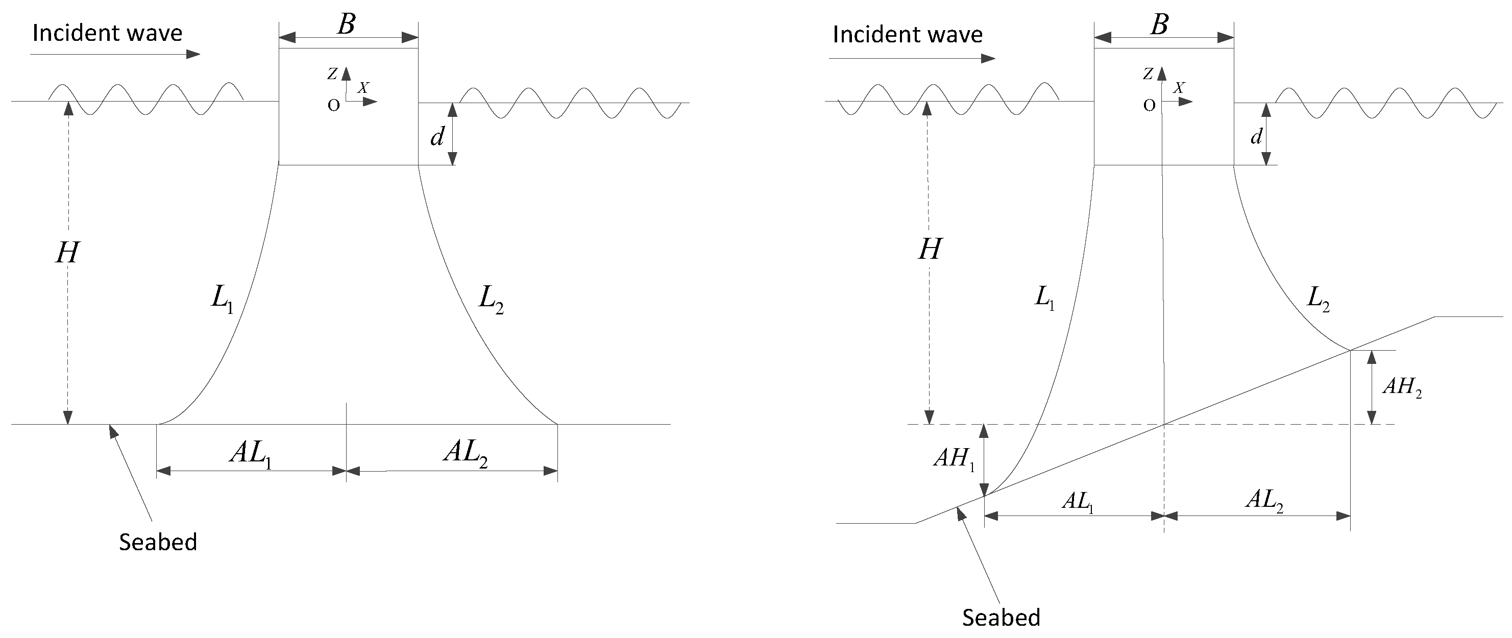Figure 9 shows the profiles of symmetrical and asymmetrical seabeds with mooring lines. For the flat seabed condition, the left-side mooring line length $L_1$ and anchor horizontal distance $A{L}_1$ equal the right-side values $L_2$ and $A{L}_2$. The average water depths H for the sloping seabeds are same as the flat ones for direct comparisons. Each mooring line has a weight of W = 5 kN/m in water and two mooring lines are used on each side in the present study unless otherwise stated.

Table 2. Parameters of four sets of mooring lines for symmetrical seabed condition with water depth $h=200$ m.

	Mooring Line Type	${\mathit{L}}_1$	${\mathit{L}}_2$	${\mathit{AL}}_1$	${\mathit{AL}}_2$
	Set 1	600 m	600 m	549 m	549 m
	Set 2	700 m	700 m	656 m	656 m
	Set 3	800 m	800 m	762 m	762 m
	Set 4	900 m	900 m	766 m	766 m

shows parameters of the four sets of mooring lines for the symmetrical seabed condition. In the present study, $10\%$ of the mooring line length are lying on the seabed for all the numerical simulations unless stated otherwise. The incident wave has a wave amplitude A = 1 m and the mooring line is kept in a catenary profile in all numerical simulations. Free decay test shows the heave nature period for this coupled body and mooring line system are 8.78 s. Figure 10 shows a comparison of floating body surge motion $RA{O}_{11}\left(\omega \right)$ between without mooring line condition, mooring line set 1, mooring line set 2, mooring line set 3 and mooring line set 4. It is observed that the mooring line reduces the surge motion $RA{O}_{11}\left(\omega \right)$ noticeably and the $RA{O}_{11}\left(\omega \right)$ becomes smaller as the mooring line length increases. Figure 11 shows a comparison of the heave motion $RA{O}_{22}\left(\omega \right)$ of the floating body between without mooring line condition, mooring line set 1, mooring line set 2, mooring line set 3 and mooring line set 4. It is noticed that the mooring line reduces the heave motion amplitude significantly. Longer mooring line generates larger restoring force for the floating body and therefore the heave motion amplitude reduces more. The peak value of motion amplitude is shifted towards the high wave frequency as the mooring line length increases. This finding is in line with that of [36].

In order to investigate the hydrodynamic effects of asymmetrical seabed and mooring line, a symmetrical mooring line set $L_1=L_2=700$ m is taken as the basis. Two asymmetrical mooring line sets are used in the numerical simulations and the parameters for these two sets of mooring lines are presented in

Table 3. Parameters of two sets of mooring lines for asymmetrical seabed condition with water depth $h=200$ m.

	Mooring Line Type	${\mathit{L}}_1$	${\mathit{L}}_2$	${\mathit{AL}}_1$	${\mathit{AL}}_2$	${\mathit{AH}}_1$	${\mathit{AH}}_2$
	Set 1	720 m	680 m	674 m	640 m	9.7 m	9.2 m
	Set 2	740 m	660 m	695 m	620 m	10.0 m	8.8 m

. For direct comparison, the total mooring line lengths are same for both symmetrical and asymmetrical mooring line sets. It should be emphasised that the floating body has to be at static equilibrium. This requirement is naturally satisfied for symmetrical mooring line set. For asymmetrical seabed and mooring line set, the left side mooring line is arranged similarly as the symmetrical case, i.e., $10\%$ of the mooring line length are laid on the seabed. The right-side mooring line has to be arranged to balance the horizontal mooring line force generated by the left side. An iterative procedure is developed to calculate the anchor horizontal distance $A{L}_2$ and the anchor vertical distance $A{H}_2$ is readily available according to the seabed slope once $A{L}_2$ is obtained. In such arrangement, the difference of vertical mooring line forces generated by the left and right sides is less than $3\%$ and has marginal effects on the pitch motion of the floating body.

Figure 12 shows a comparison of the surge motion $RA{O}_{11}\left(\omega \right)$ of the floating body between symmetrical mooring line condition, asymmetrical mooring line set 1 and set 2. It is noticed that the surge motion $RA{O}_{11}$ reduces appreciably as the asymmetry level increases across the whole wave frequency range. Compared with the symmetrical case, the left-side length of asymmetrical mooring line set 2 increases by $6\%$, but it reduces the $RA{O}_{11}$ by approximately $15\%$. If less mooring line length is allowed to lie on the seabed, effects due to the mooring line asymmetry are expected to be more significant. It should be noticed that the difference between the left-and right-side mooring lines is in a reasonable range, otherwise the mooring line set can not keep the floating body at a static equilibrium position. The heave motion $RA{O}_{22}\left(\omega \right)$ is marginally affected by the asymmetrical mooring line setup and therefore the data are not presented here.

Numerical simulations are further performed for the floating body positioned in a water depth of $H=20$ m. Both flat seabed with symmetrical mooring lines and sloping seabed with asymmetrical mooring lines are considered. The mooring lines on the sloping seabed have length $L_1=L_2$ but are arranged in asymmetrical position. These mooring lines are lying on flat seabed portion whereas sloping seabed portion is located within two anchor points. Both the symmetrical and asymmetrical mooring line configurations have the same length $L_1=L_2=60$ m for direct comparison. The $15\%$ mooring line length is allowed to lie on the seabed for both cases. Figure 13 shows the profile of an asymmetrical seabed with mooring lines positioned in the water depth $H=20$ m.

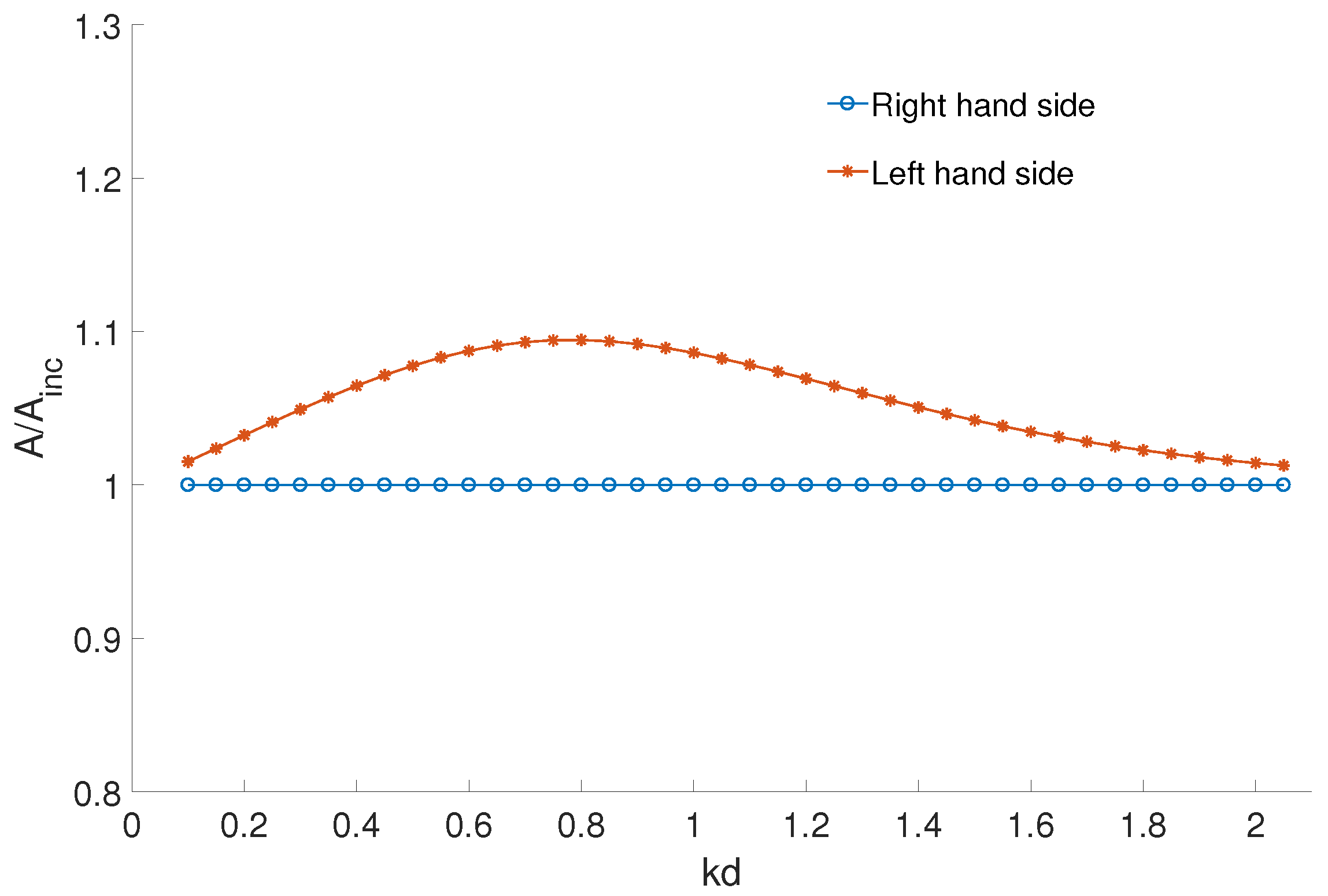
The sloping seabed effect for the incident wave amplitude is first investigated, and no floating body or mooring lines are included in the fluid domain. A linear incident wave with a wave amplitude of $A_{inc}$ comes from the left-hand side and moves towards the right-hand side as illustrated in Figure 13. Figure 14 shows the incident wave amplitude A on the right- and left-hand sides over a sloping seabed with sloping angle $\tan \theta =1/8$. The left-hand side has a wave amplitude of $A=A_{inc}$ as the incident wave comes from the left. The wave amplitude changes gradually on the sloping part due to the sloping seabed effects. The wave becomes steady when it moves into the flat part on the right-hand side. It is noticed that the incident wave amplitude increases due to the sloping seabed and the sloping seabed has largest effect for the incident wave when the wave frequency is approximately $kd=0.8$.

The left-side mooring line weight has a weight of W = 5 kN/m in water for the sloping seabed case, and the floating body is at a static equilibrium. A preliminary iterative procedure is developed to calculate the right-side mooring line weight per meter to reach static equilibrium. Figure 15 shows a comparison of the surge motion $RA{O}_{11}\left(\omega \right)$ of the floating body between a flat seabed and a sloping seabed with $\tan \theta =1/20$, $\tan \theta =1/10$ and $\tan \theta =1/8$, respectively. It is noticed that the surge motion $RA{O}_{11}\left(\omega \right)$ is smaller for the flat seabed than the sloping seabed conditions and $RA{O}_{11}\left(\omega \right)$ increases as the sloping seabed angle $\theta$ increases across the frequency range.

Figure 16 shows a comparison of the heave motion $RA{O}_{22}\left(\omega \right)$ of the floating body between flat seabed, sloping seabed with $\tan \theta =1/20$, $\tan \theta =1/10$ and $\tan \theta =1/8$, respectively. It is noticed that the peak responses of the heave motion $RA{O}_{22}\left(\omega \right)$ are shifted towards lower wave frequency and the peak response values increase along with the sloping seabed angle. The phenomenon presented in Figure 15 and Figure 16 implies that the sloping seabed with asymmetrical mooring line arrangement produces less mooring stiffness than does the symmetrical case. In the preliminary study to investigate the right-side mooring weight, numerical simulations show that less weight is required compared with the left side.

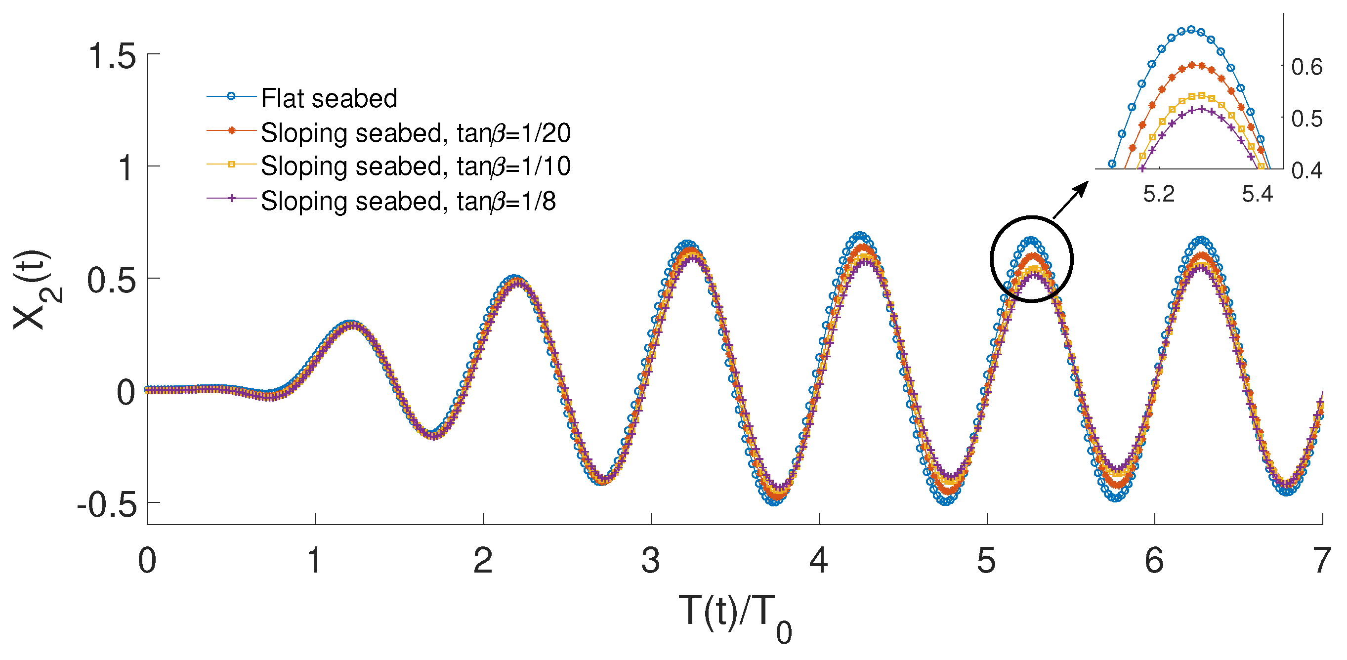
Figure 17 shows a comparison of the time record of the floating-body heave motion $X_2\left(t\right)$ for wave frequency $kd=1.0$ between flat seabed, sloping seabed with $\tan \theta =1/20$, $\tan \theta =1/10$ and $\tan \theta =1/8$, respectively. The heave motion $X_2\left(t\right)$ has the largest amplitude for flat seabed condition and the $X_2\left(t\right)$ motion amplitudes decrease as the sloping angles increase. These time-domain results are aligned with those frequency-domain results presented in Figure 16. In this study, the fluid domain is described by a linear boundary element model. The peak value for heave motion $X_2\left(t\right)$ is around $0.7$ whereas the trough value is about $0.5$. This nonharmonic body motion track demonstrates the nonlinear characteristics of the coupled floating body-mooring line system.

Figure 18 shows a comparison of mooring line force $F_2^{mooring}\left(t\right)$ for wave frequency $kd=1.0$ between flat seabed, sloping seabed with $\tan \theta =1/20$, $\tan \theta =1/10$ and $\tan \theta =1/8$, respectively. The mooring line pretension is excluded in the mooring line force $F_2\left(t\right)$. The mooring line force $F_2^{mooring}\left(t\right)$ has the largest amplitude for flat seabed condition and $F_2^{mooring}\left(t\right)$ amplitudes decrease as the sloping angles increase. It is also noticed that the force peak values are smaller than the trough values and this phenomenon is due to the fact that the heave motion $X_2\left(t\right)$ peak values are bigger than the trough values. Figure 19 demonstrates a comparison of time record of floating body surge motion $X_1\left(t\right)$ for wave frequency $kd=1.0$ between flat seabed, sloping seabed with $\tan \theta =1/20$, $\tan \theta =1/10$ and $\tan \theta =1/8$, respectively. The surge motion $X_1\left(t\right)$ peak values are almost same for these different seabed conditions but the $X_1\left(t\right)$ has the least value for flat seabed condition. It is also noticed that the nonlinear characteristics become more obvious as the seabed inclination increases.

Figure 20 shows the wave force $F_2^{wave}\left(\omega \right)$ on the moored body excited by an incident wave for the slope seabed angle of $tan\theta =1/8$. It is noticeable that the wave force $F_2^{wave}\left(\omega \right)$ increases with the wave frequency for $kd<0.6$. This wave force $F_2^{wave}\left(\omega \right)$ reaches its peak in the period $0.6<kd<0.7$ and decreases gradually with the wave frequency for $kd>0.7$. This variation trend is in line with the moored body motion as presented in Figure 16.

To demonstrate the slope seabed inclination effects for the mooring line force. Numerical simulations are performed for this floating body positioned above a sloping seabed with various inclinations. Figure 21 shows a comparison of the mooring line force $F_2^{mooring}$ amplitude for different slope seabed angle $\tan \theta$ for the floating body experiencing an incident wave with frequency $kd=1.0$. It is noticed that the mooring line force $F_2^{mooring}$ reduces as seabed angle $\tan \theta$ increases. In the present study, the mooring line and floating body are coupled into an integrated model. The mooring line force is excited mainly due to the floating body motion which is caused by the incident wave. The mooring line force amplitude conforms with the floating body motion amplitude.

It should be noticed that the coupled floating body and mooring line system natural frequency is within the wave frequency range and only the wave-frequency responses are investigated in this paper. The low-frequency responses are very important for large floating bodies.

5. Conclusions

A two-dimensional coupled floating body-mooring line model is developed to study the freely floating body motion responses in both flat and sloping seabed conditions. A continuous Rankine source based boundary element model is established to describe the fluid domain. This model comprises three time-domain boundary integral equations accounting for diffraction problem, radiation problem and reflection problem, respectively. The mooring line is formulated by a catenary mooring line model and coupled with the boundary element model at each time step.

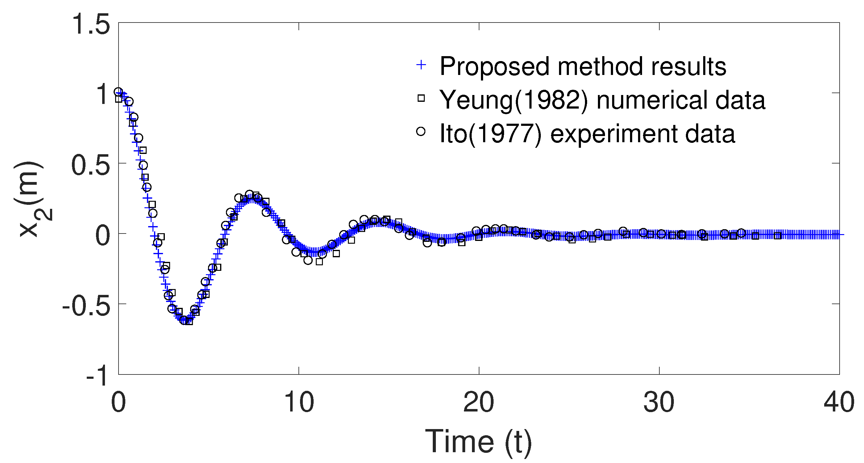
Numerical validations were carried out for the static offset test, free decay test without mooring line, free decay test with mooring line and regular wave simulation. Reasonable agreement with published data demonstrates the accuracy of proposed model.

Two numerical cases are investigated with an emphasis on the hydrodynamic effects of sloping seabed and asymmetrical mooring line. In the first numerical study, both the surge motion $RA{O}_{11}$ and the heave motion $RA{O}_{22}$ decrease as the mooring line length increases for flat seabed condition. For the sloping seabed case, the left and right sides of mooring line have different lengths and are laid on sloping seabed portion. The right-side mooring line is positioned to keep the floating body at static equilibrium. Numerical results show that the surge motion $RA{O}_{11}$ decreases as the asymmetrical level increases across the whole frequency range but the heave motion $RA{O}_{22}$ keeps constant regardless of the asymmetry level. These numerical findings indicate that in such sloping seabed conditions, the mooring line system shows better station-keeping capability than it does in flat seabed conditions.

For the second numerical case, both the left and right sides of mooring lines are laid on flat seabed portion with sloping portion between two anchor points. The left and right mooring line has same length but different weight to keep the floating body in static equilibrium position. Numerical study shows that both the surge motion $RA{O}_{11}$ and heave motion $RA{O}_{22}$ increase as the sloping seabed angle becomes larger. The coupled floating body-mooring line system demonstrates nonlinear characteristics for the body motion and mooring line force responses in the time domain. The surge motion has clearer nonlinear performance than the heave motion. An asymmetrical mooring line configuration demonstrates less station-keeping capability than an symmetrical configuration, but it also requires less mooring line weight and steel consumption. From an economical viewpoint, such a mooring line configuration could be beneficial. In actual industrial projects, the design of asymmetrical mooring line is a trade-off between station-keeping capability and economical benefit.

This paper deals with two-dimensional cases and therefore has academic values, while practical engineering problems are three-dimensional. The study of three-dimensional coupled floating body-mooring line problem and an extention to wave energy converters will be part of our future work.

References

1. Lefebvre, S.; Collu, M. Preliminary design of a floating support structure for a 5 MW offshore wind turbine. Ocean Eng. 2012, 40, 15–26. [Google Scholar] [CrossRef]
2. Ardianti, A.; Mutsuda, H.; Kawawaki, K.; Doi, Y. Fluid structure interactions between floating debris and tsunami shelter with elastic mooring caused by run-up tsunami. Coast. Eng. 2018, 137, 120–132. [Google Scholar] [CrossRef]
3. Jiang, Z.; Moan, T.; Gao, Z. A comparative study of shutdown procedures on the dynamic responses of wind turbines. J. Offshore Mech. Arctic Eng. 2015, 137, 011904. [Google Scholar] [CrossRef]
4. Zanuttigh, B.; Angelelli, E. Experimental investigation of floating wave energy converters for coastal protection purpose. Coast. Eng. 2013, 80, 148–159. [Google Scholar] [CrossRef]
5. Li, L.; Jiang, Z.; Høiland, A.V.; Ong, M.C. Numerical analysis of a vessel-shaped offshore fish farm. J. Offshore Mech. Arctic Eng. 2018, 140. [Google Scholar] [CrossRef]
6. Bai, K. The added mass of two-dimensional cylinders heaving in water of finite depth. J. Fluid Mech. 1977, 81, 85–105. [Google Scholar] [CrossRef]
7. Xiong, L.; Lu, H.; Yang, J.; Zhao, W. Motion responses of a moored barge in shallow water. Ocean Eng. 2015, 97, 207–217. [Google Scholar] [CrossRef]
8. Feng, A.; Bai, W.; You, Y.; Chen, Z.; Price, W. A Rankine source method solution of a finite depth, wave-body interaction problem. J. Fluids Struct. 2016, 62, 14–32. [Google Scholar] [CrossRef] [Green Version]
9. Buchner, B. The motions of a ship on a sloped seabed. In Proceedings of the 25th International Conference on Offshore Mechanics and Arctic Engineering, Hamburg, Germany, 4–9 June 2006; pp. 339–347. [Google Scholar]
10. Ferreira, M.; Newman, J. Diffraction effects and ship motions on an artificial seabed. In Proceedings of the 24th International Workshop on Water Waves and Floating Bodies, Zelenogorsk, Russia, 19–22 April 2009. [Google Scholar]
11. Belibassakis, K.; Athanassoulis, G. Three-dimensional Green’s function for harmonic water waves over a bottom topography with different depths at infinity. J. Fluid Mech. 2004, 510, 267–302. [Google Scholar] [CrossRef]
12. Belibassakis, K. A boundary element method for the hydrodynamic analysis of floating bodies in variable bathymetry regions. Eng. Anal. Bound. Elements 2008, 32, 796–810. [Google Scholar] [CrossRef]
13. Kim, T.; Kim, Y. Numerical analysis on floating-body motion responses in arbitrary bathymetry. Ocean Eng. 2013, 62, 123–139. [Google Scholar] [CrossRef]
14. Feng, A.; Cai, H.; You, Y. Freely floating body motion responses induced by wave and current in seabed conditions. Ocean Eng. 2019, 172, 396–406. [Google Scholar] [CrossRef]
15. Feng, A.; Magee, A.; Price, W. Two dimensional wave-current-structure interaction with flat or sloping seabed environment in a linearized framework. Ocean Eng. 2019, 174, 296–306. [Google Scholar] [CrossRef]
16. Li, L.; Jiang, Z.; Ong, M.C.; Hu, W. Design optimization of mooring system: An application to a vessel-shaped offshore fish farm. Eng. Struct. 2019, 197, 109363. [Google Scholar] [CrossRef]
17. Mavrakos, S.; Papazoglou, V.; Triantafyllou, M.; Hatjigeorgiou, J. Deep water mooring dynamics. Mar. Struct. 1996, 9, 181–209. [Google Scholar] [CrossRef]
18. Montasir, O.; Yenduri, A.; Kurian, V. Effect of mooring line configurations on the dynamic responses of truss spar platforms. Ocean Eng. 2015, 96, 161–172. [Google Scholar] [CrossRef]
19. Smith, R.; MacFarlane, C. Statics of a three component mooring line. Ocean Eng. 2001, 28, 899–914. [Google Scholar] [CrossRef]
20. Yuan, Z.; Incecik, A.; Ji, C. Numerical study on a hybrid mooring system with clump weights and buoys. Ocean Eng. 2014, 88, 1–11. [Google Scholar] [CrossRef] [Green Version]
21. Lie, H. MIMOSA, a Computation Program for Mooring and Stationkeeping Analysis, User’s Manual; Technical Report; MARINTEK: Trondheim, Norway, 1990. [Google Scholar]
22. Larsen, K.; Sandvik, P. Efficient methods for the calculation of dynamic mooring line tension. In Proceedings of the 1st ISOPE European Offshore Mechanics Symposium, Trondheim, Norway, 20–22 August 1990. [Google Scholar]
23. Ormberg, H.; Passano, E. RIFLEX Theory Manual; Technical Report; MARINTEK: Trondheim, Norway, 2012. [Google Scholar]
24. Kim, M.; Koo, B.; Mercier, R.; Ward, E. Vessel/mooring/riser coupled dynamic analysis of a turret-moored FPSO compared with OTRC experiment. Ocean Eng. 2005, 32, 1780–1802. [Google Scholar] [CrossRef]
25. Hall, M.; Goupee, A. Validation of a lumped-mass mooring line model with DeepCwind semisubmersible model test data. Ocean Eng. 2015, 104, 590–603. [Google Scholar] [CrossRef] [Green Version]
26. Ran, Z.; Kim, M. Nonlinear coupled responses of a tethered spar platform in waves. Int. J. Offshore Polar Eng. 1997, 7, 1–8. [Google Scholar]
27. Girón, A.R.C.; Corrêa, F.N.; Hernández, A.O.V.; Jacob, B.P. An integrated methodology for the design of mooring systems and risers. Mar. Struct. 2014, 39, 395–423. [Google Scholar] [CrossRef]
28. Molen, W.; Wenneker, I. Time-domain calculation of moored ship motions in nonlinear waves. Coast. Eng. 2008, 55, 409–422. [Google Scholar] [CrossRef]
29. Faltinsen, O. Sea Loads on Ships and Offshore Structures; Cambridge University Press: Cambridge, UK, 1990. [Google Scholar]
30. Feng, A.; Price, W. Numerical simulations of the hydrodynamic responses of a body interacting with wave and current over a sloping seabed. Appl. Ocean Res. 2018, 79, 184–196. [Google Scholar] [CrossRef]
31. Yeung, R. The transient heaving motion of floating cylinders. J. Eng. Math. 1982, 16, 97–119. [Google Scholar] [CrossRef]
32. Ito, S. Study of the Transient Heave Oscillation of a Floating Cylinder. Master’s Thesis, Massachusetts Institute of Technology, Cambridge, MA, USA, 1977. [Google Scholar]
33. Patel, M. Dynamics of Offshore Structures; Butterworth-Heinemann: Oxford, UK, 1989. [Google Scholar]
34. Ren, B.; He, M.; Dong, P.; Wen, H. Nonlinear simulations of wave-induced motions of a freely floating body using WCSPH method. Appl. Ocean Res. 2015, 50, 1–12. [Google Scholar] [CrossRef]
35. Martin, T.; Bihs, H.; Kamath, A.; Arntsen, Ø. Arntsen, Simulation of Floating Bodies in Waves and Mooring in a 3D Numerical Wave Tank Using REEF3D. In Proceedings of the 4th International Conference in Ocean Engineering, Chennai, India, 18–21 February 2018; pp. 673–683. [Google Scholar]
36. Bian, S.; Xiang, S. Manage tensioner stroke for dry tree semisubmersibles. In Proceedings of the 32nd International Conference on Ocean, Offshore and Arctic Engineering, Nantes, France, 9–14 June 2013; pp. 1–9. [Google Scholar]
Figure 1. Sketch of a catenary mooring line model.
Jmse 08 00389 g001
Figure 2. Illustration of a coupled floating body-mooring line model with a seabed condition.
Jmse 08 00389 g002
Figure 3. Definitions and illustration of the floating body-mooring line problem.
Jmse 08 00389 g003
Figure 4. Comparison of mooring line stiffness with respect to horizontal force T x ( a ) and vertical force T z ( b ) between proposed numerical method and numerical data of [29].
Jmse 08 00389 g004
Figure 5. Comparison of heave decay test for the semi circular cylinder between proposed method results, [31] numerical results and [32] experimental data.
Jmse 08 00389 g005
Figure 6. Surge decay test for cylinder with mooring line stiffness K 1 = 90 , 000 N/m, 135 , 000 N/m, 180 , 000 N/m and 225 , 000 N/m, respectively.
Jmse 08 00389 g006
Figure 7. Comparison of time records of surge motion X 1 ( t ) (a) and heave motion X 2 ( t ) (b) between proposed method results and [34] experimental data and [35] numerical data without mooring effect.
Jmse 08 00389 g007
Figure 8. Comparison of time records of surge motion X 1 ( t ) (a) and heave motion X 2 ( t ) (b) between proposed method results and [35] numerical data with mooring effect included.
Jmse 08 00389 g008
Figure 9. Profiles of symmetrical and asymmetrical seabeds with mooring lines.
Jmse 08 00389 g009
Figure 10. Comparison of the floating body surge motion R A O 11 ( ω ) between without mooring line condition, mooring line set 1, mooring line set 2, mooring line set 3 and mooring line set 4.
Jmse 08 00389 g010
Figure 11. Comparison of the floating body heave motion R A O 22 ( ω ) between without mooring line condition, mooring line set 1, mooring line set 2, mooring line set 3 and mooring line set 4.
Jmse 08 00389 g011
Figure 12. Comparison of the floating body surge motion R A O 11 ( ω ) between symmetrical mooring line condition, asymmetrical mooring line set 1 and set 2.
Jmse 08 00389 g012
Figure 13. Profile of asymmetrical seabed with mooring lines positioned in water depth H = 20 m.
Jmse 08 00389 g013
Figure 14. Incident wave amplitude A on the right hand and left hand sides over a sloping seabed with sloping angle tan θ = 1 / 8 .
Jmse 08 00389 g014
Figure 15. Comparison of the floating body surge motion R A O 11 ( ω ) between flat seabed, sloping seabed with tan θ = 1 / 20 , tan θ = 1 / 10 and tan θ = 1 / 8 , respectively with mooring line length L 1 = L 2 = 60 m.
Jmse 08 00389 g015
Figure 16. Comparison of the floating body heave motion R A O 22 ( ω ) between flat seabed, sloping seabed with tan θ = 1 / 20 , tan θ = 1 / 10 and tan θ = 1 / 8 , respectively with mooring line length L 1 = L 2 = 60 m.
Jmse 08 00389 g016
Figure 17. Comparison of time record of floating body heave motion X 2 ( t ) for wave frequency k d = 1.0 between flat seabed, sloping seabed with tan θ = 1 / 20 , tan θ = 1 / 10 and tan θ = 1 / 8 , respectively.
Jmse 08 00389 g017
Figure 18. Comparison of time record of mooring line force F 2 ( t ) for wave frequency k d = 1.0 between flat seabed, sloping seabed with tan θ = 1 / 20 , tan θ = 1 / 10 and tan θ = 1 / 8 , respectively.
Jmse 08 00389 g018
Figure 19. Comparison of time record of floating body surge motion X 1 ( t ) for wave frequency k d = 1.0 between flat seabed, sloping seabed with tan θ = 1 / 20 , tan θ = 1 / 10 and tan θ = 1 / 8 , respectively.
Jmse 08 00389 g019
Figure 20. Wave force F 2 w a v e ( ω ) on the moored body excited by an incident wave.
Jmse 08 00389 g020
Figure 21. Comparison of the mooring line force F 2 m o o r i n g amplitude for different slope seabed angle tan θ for floating body experiencing an incident wave with frequency k d = 1.0 .
Jmse 08 00389 g021